| Issue |
A&A
Volume 690, October 2024
|
|
|---|---|---|
| Article Number | A97 | |
| Number of page(s) | 15 | |
| Section | Galactic structure, stellar clusters and populations | |
| DOI | https://doi.org/10.1051/0004-6361/202450782 | |
| Published online | 02 October 2024 | |
The AMBRE Project: Lead abundance in Galactic stars
1
Université Côte d’Azur, Observatoire de la Côte d’Azur, CNRS, Laboratoire Lagrange,
Bd de l’Observatoire, CS 34229,
06304
Nice cedex 4,
France
2
Institut für Kernphysik, Technische Universität Darmstadt,
Schlossgartenstr. 2,
Darmstadt
64289,
Germany
3
I.N.A.F. Osservatorio Astronomico di Trieste,
via G.B. Tiepolo 11,
34131
Trieste,
Italy
4
Dipartimento di Fisica, Sezione di Astronomia, Università di Trieste,
Via G. B. Tiepolo 11,
34143
Trieste,
Italy
5
I.N.F.N. Sezione di Trieste,
via Valerio 2,
34134
Trieste,
Italy
6
I.N.A.F. Osservatorio Astronomico d’Abruzzo, via Maggini snc,
64100
Teramo,
Italy
7
I.N.F.N. Sezione di Perugia, via Pascoli snc,
06123
Perugia,
Italy
★ Corresponding author; e-mail: This email address is being protected from spambots. You need JavaScript enabled to view it.
Received:
18
May
2024
Accepted:
5
August
2024
Abstract
Context. The chemical evolution of neutron capture elements in the Milky Way is still a matter of debate. Although more and more studies investigate their chemical behaviour, there is still a lack of a significant large sample of abundances of a key heavy element: lead.
Aims. Lead is the final product of the s-process nucleosynthesis channel and is one of the most stable heavy elements. The goal of this article is to present the largest catalogue of homogeneous Pb abundances, in particular for metallicities higher than −1.0 dex, and then to study the lead content of the Milky Way.
Methods. We analysed high-resolution spectra from the ESO UVES and FEROS archives. Atmospheric parameters were taken from the AMBRE parametrisation. We used the automated abundance method GAUGUIN to derive lead abundances in 653 slow-rotating FGK-type stars from the 368.34 nm Pb I line.
Results. We present the largest catalogue of Local Thermodynamic Equilibrium (LTE) and non-LTE lead abundances ever published with metallicities ranging from −2.9 to 0.6 dex and [Pb/Fe] from −0.7 to 3.3 dex. Within this sample, no lead-enhanced Asymptotic Giant Branch (AGB) stars were found, but nine lead-enhanced metal-poor stars ([Pb/Fe] > 1.5) were detected. Most of them were already identified as carbon-enhanced metal-poor stars with enrichments in other s-process species. The lead abundance of 13 Gaia Benchmark Stars are also provided. We then investigated the Pb content of the Milky Way disc by computing vertical and radial gradients and found a slightly decreasing [Pb/Fe] radial trend with metallicity. This trend together with other related ratios ([Pb/Eu], [Pb/Ba], and [Pb/α]) are interpreted thanks to chemical evolution models. The two-infall model closely reproduces the observed trends with respect to the metallicity. It is also found that the AGB contribution to the Pb Galactic enrichment has to be strongly reduced. Moreover, the contribution of massive stars with rather high rotational velocities should be favoured in the low-metallicity regime.
Key words: stars: abundances / stars: AGB and post-AGB / Galaxy: abundances / Galaxy: disk / Galaxy: evolution / Galaxy: stellar content
© The Authors 2024
 Open Access article, published by EDP Sciences, under the terms of the Creative Commons Attribution License (https://creativecommons.org/licenses/by/4.0), which permits unrestricted use, distribution, and reproduction in any medium, provided the original work is properly cited.
This article is published in open access under the Subscribe to Open model. This email address is being protected from spambots. You need JavaScript enabled to view it. to support open access publication.
1 Introduction
The nucleosynthesis of elements heavier than iron cannot occur by charged particle reactions; it is mainly carried out via neutron capture. According to the seminal work of Burbidge et al. (1957), neutron capture occurs through two processes: the slow (s-) process and the rapid (r-) process. The latter takes place at high neutron densities and short timescales (compared to β decay). Several neutrons are added before multiple α and β−decays allowing the isotope to find stability.
The different sites of r-element production are still not clearly identified. Among the different scenarios, one can find mergers of compact objects (neutron stars and/or neutron star–black hole; e.g. Freiburghaus et al. 1999; Surman et al. 2008; Thielemann et al. 2017) as well as winds from type II Supernovae (SNIIe; Woosley et al. 1994) and rare and energetic magneto-rotational SNe (MR-SNe; Winteler et al. 2012; Reichert et al. 2023).
On the contrary, the s-process occurs on longer timescales and with lower neutron densities. The main production sites for these s-elements, in particular the late evolutionary stages of low- and intermediate-mass stars, are better known, although their actual production rates are still debated.
The abundance distribution of elements formed by the s-process as a function of atomic number shows three peaks: one around Sr-Y-Zr, one around Ba-La-Ce, and one around Pb-Bi. The isotopes of lead and bismuth are the most stable ones formed by the s-process. For instance, one of the most stable Pb isotopes is 208Pb (Z = 82, N1 = 126) because the neutron and proton shells are closed, reducing the cross-section to the next neutron capture.
In this context, each s-process peak is associated with a different source. The main sources are rotating massive stars and Asymptotic Giant Branch (AGB) stars. First, elements with an atomic mass number (A) between about 60 and 90 are thought to be formed through the weak-s process during the He-core burning phase of massive stars (M ≳ 8 M⊙). This happens through the 22Ne(α,n)25Mg reaction [Cameron 1960, Iben and Renzini 1983]. When the helium runs out, the 22Ne is only partially consumed and neutron production continues in the convective carbon layer (Couch et al. 1974; Kappeler et al. 1989; Pignatari et al. 2010; Käppeler et al. 2011). This 22Ne comes from the 14N produced during the hydrogen combustion phase in the core via the CNO cycle. We note that these s-process elements are not altered by the final explosive nucleosynthesis of SNIIe and enrich the interstellar medium (ISM) (e.g. Kappeler et al. 1989; Prantzos et al. 1990; Limongi & Chieffi 2018).
The main-s component is responsible for the production of heavier elements with 90 ≲ A ≲ 204 during the thermal pulse phases of low- and intermediate-mass stars in the last stage of their evolution (AGB with 1.3 M⊙ ≲ M ≲ 8⊙) (Arlandini et al. 1999; Busso et al. 1999). The protons left by the receding of the convective envelope are captured by the 12C present in the He-intershell between two thermal pulses (the interpulse). This produces 13C via the reaction 12C(p, γ) 13N(β+, ν) 13C and forms a thin pocket of 13C. The latter is itself converted to oxygen via the 13C(α, n) 16O reaction, thus producing a source of neutrons for the s-process Straniero et al. (1995). Since the 13C pocket is partially covered by a layer of 14N and 22Ne (14N acts as a poison for neutrons due to the 14N(n,p) 14C reaction), the s-process takes place in the deepest part of this 13C pocket where little 14N is found (Cristallo et al. 2009b). For intermediate-mass stars (M ≳ 3 M⊙), the temperature at the base of the convective zone is higher and a second neutron source is activated: the 22Ne(α,n)25Mg reaction. This source is marginal in low-mass AGBs of solar metallicity. It is important to note that stellar metallicity and rotation have a large impact on the efficiency of these nucleosynthesis channels (Cristallo et al. 2009b, 2011; Karakas & Lattanzio 2014).
However, neither the weak nor the main s-process is sufficient to explain the observed lead abundances (Pb, Z2 = 82) in the Solar System. Therefore, a new process (called the strong s-process) was introduced (Kappeler et al. 1989), in line with the proposition of Clayton & Rassbach (1967) that the Solar System lead is not formed by the r-process. Later studies on AGB nucleosynthesis and yields indeed confirmed that Pb production in low-mass and low-metallicity stars corresponds to this strong s-process (Gallino et al. 1998; Goriely & Mowlavi 2000; Busso et al. 2001; Choplin et al. 2022), whose source is still not well identified.
Furthermore, observational studies of lead abundances in stellar atmospheres are not very common, mainly because of the difficulty obtaining reliable results, due to the complexity of the spectral domain in which the main (and weak) atomic transitions of Pb reside. We note that most of the studies related below deal with metal-poor stars enriched in carbon (known as CEMP stars). These stars are probably affected by mass transfer from an AGB companion that previously produced carbon and neutron-capture elements. Among the main Pb studies, one can cite the work of Van Eck et al. (2001) who analysed three metal-poor stars (HD 187861, HD 196944, and HD 224959) with very high Pb abundances. This study was completed by the analysis of two other Pb-rich stars (Van Eck et al. 2003). Independently, Jonsell et al. (2006), Lucatello et al. (2003), Sivarani et al. (2004), Ivans et al. (2005), and Barbuy et al. (2011) added a few new Pb-rich stars to this list. Most of these stars are very metal-poor ([M/H] < −2.0 dex), highlighting again the s-process contribution of low-metallicity environments.
Independently, Aoki et al. (2002) studied eight metal-poor (−2.7 < [Fe/H] < −1.9 dex) carbon-rich stars and found a strong dispersion of [Pb/Ba]. Allen & Barbuy (2006) studied 26 Ba-type stars, enriched in r-elements and Pb. Roederer et al. (2009) determined Pb (and other heavy element) abundances for 27 metal-poor stars (−3.1 < [Fe/H] < −1.4 dex) with heavy element enrichments. Finally, Roederer et al. (2014) provided a catalogue of 13 metal-poor stars for which atmospheric parameters and abundances (including some Pb abundances) are provided. Non Local Thermodynamic Equilibrium (NLTE) corrections for some Pb lines were also provided by Mashonkina et al. (2012). More recently, Roederer et al. (2020) and Peterson (2021) determined Pb abundances for three and four stars, respectively, based on the analysis of UV lines. Finally, we recall that De Smedt et al. (2015, 2016) also reported Pb abundances in some post-AGB stars. Lastly, we recall that Prantzos et al. (2018) published Galactic chemical evolution models of [Pb/Fe] versus [Fe/H]. As can be seen in their Fig. 16, there is a clear paucity of observational data, especially at metallicities higher than −1.0.
In this work, we provide Pb abundances within the context of the AMBRE Project (de Laverny et al. 2013). AMBRE has parametrised ESO archived stellar spectra (FEROS, UVES, and HARPS), thanks to the MATISSE algorithm (Recio-Blanco et al. 2006) trained with a specific synthetic spectrum grid (de Laverny et al. 2012). Within AMBRE, chemical abundances are derived using the GAUGUIN optimisation method (see Sec. 2.1 and Bijaoui 2012; Recio-Blanco et al. 2016, for a detailed description) as already performed, for instance, for the determination of Li, r-process, Mg, and S chemical abundances (Guiglion et al. 2016, 2018; Santos-Peral et al. 2020; Perdigon et al. 2021, respectively)3. The initial goal of AMBRE was to test both algorithms, MATISSE and GAUGUIN, on large spectra datasets and to develop an optimal stellar parametrisation pipeline for the analysis of Gaia Radial Velocity Spectrometer data by the DPAC/GSP-spec module (Recio-Blanco et al. 2023). The adopted methodology for lead abundance estimations is presented in Sec. 2, while Sec. 3 describes the AMBRE:Pb catalogue. Section 4 discusses Pb abundances in some peculiar stars, including the Gaia Benchmark Stars, and Sec. 5 explores the lead abundance properties in the Milky Way. Our conclusions are summarised in Sec. 6.
2 Derivation of lead abundances
For this study, we adopted the classical AMBRE methodology, basically the abundance determination thanks to the GAUGUIN method and a specific synthetic reference spectra grid with varying Pb abundances, for the determination of lead abundances.
Several lead lines were previously analysed in stellar spectra. For instance, in the ultraviolet domain (not covered by the AMBRE spectra), the Pb II 220.35 nm was adopted by Roederer et al. (2020) in three metal-poor stars, whereas the Pb I 283.305 nm was analysed by Roederer et al. (2009), Roederer et al. (2016) and Peterson (2021) in 27, one and four metal-poor stars, respectively. Other lead lines in the optical domain such as the 363.95, 373.99, 405.78 and 722.89 nm transitions were also analysed to derive the Pb solar abundance (de Jager & Neven 1962; Grevesse 1969; Hauge & Sørli 1973, for instance). Nevertheless, all those atomic transitions are severely blended or very faint in the solar-type stellar spectra. To avoid such problems, we have therefore selected the Pb I line at 368.346 nm, one of the less blended lines in cool star (particularly dwarfs) spectra and the most accurate one for deriving lead abundance in the Sun (e.g. Asplund et al. 2009; Grevesse et al. 2015; Asplund et al. 2021). For this line, we adopted the atomic line data of Biémont et al. (2000, see Sect. 2.3 for more details). Some example observed spectra around the selected Pb I line are shown in Fig. 1.
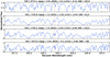 |
Fig. 1 Identification of the selected Pb I line (red vertical line) in some AMBRE example spectra. |
2.1 Lead abundances determination with GAUGUIN
Briefly, to derive chemical abundances, GAUGUIN first builds a set of reference spectra with varying lead abundances for the atmospheric parameter of the analysed star (hereafter called the 1D grid). These parameters (Teff, log(g), [M/H]4 and [α/Fe]) are provided by the AMBRE parametrisation. The reference spectra of the 1D grid are interpolated from a 5D grid (four atmospheric parameters plus [Pb/Fe]) of synthetic spectra, described hereafter. Then, the observed spectra are automatically normalised over ~4 nm and a second normalisation is performed over a smaller range around the line (~0.06 nm in our case) to locally readjust the continuum (Santos-Peral et al. 2020). Finally, the minimum of the quadratic distances between the observed and reference spectra is calculated over a spectral range of 0.02 nm around the lead line. This provides the initial guess of the lead abundance, from which the Gauss-Newton algorithm derives the final solution in a similar way as implemented for the Gaia/GSP-spec pipeline (Recio-Blanco et al. 2023).
Together with the chemical abundances, GAUGUIN also provides a value for the upper limit of the abundance below which the line cannot be detected. This upper limit is mainly dependent on the atmospheric parameters and the signal-to-noise ratio (S/N) which is also estimated by the AMBRE parametrisation. It is used to reject weak and/or doubtful detections. Moreover, for each spectrum, a white Gaussian noise (whose standard deviation is proportional to the S/N of the input spectrum) was computed for 1000 realisations and added to the initial spectrum. GAUGUIN then determined the lead abundance for each realisation, leading to 1000 abundances for each spectrum. We then calculated the median value (represented by the quantile 50, Q50, and adopted as the lead abundance hereafter) as well as the quantiles Q84 and Q16 which can be used to estimate the error associated with the determination of lead abundances (see Sec. 3.3).
2.2 Observed spectra
As described above, our method compares observed and synthetic reference spectra. Both sets of spectra have thus to be adapted in order to have similar spectral resolution and wavelength sampling.
First, we have selected AMBRE spectra covering the selected Pb I line. Our sample of spectra were collected with the FEROS and UVES spectrographs (BLUE346 and BLUE390 setups) already parametrised within the AMBRE Project (Worley et al. (2012) and Worley et al. (2016) respectively). We first selected spectra having a S/N > 20, 3500 K < Teff < 8000 K, 0.0 < log(g) < 5.5 (g in cm/s2) and whose AMBRE Quality Flag is 0 or 1 (i.e. good or very good parametrisation; following the AMBRE flagging criteria). This led to an initial sample of 5998 FEROS spectra plus 1508 and 1202 UVES spectra of the BLUE346 and BLUE390 setups, respectively. GAUGUIN thus analysed a total of 8708 stellar spectra times the number of Monte-Carlo S/N realisations (about 8.7 million spectra in total). We note that the corresponding number of stars is much smaller because of the presence of several repeated spectra for several stars (see below).
To be able to perform the chemical analysis, the observed spectra were first corrected for radial velocity shifts (whose value is also provided by the AMBRE parametrisation) and a spectral domain of 4 nm around the lead line was selected. As the spectral resolutions of the FEROS and UVES spectra slightly differ (R ~ 48 000 and R ~ 40000, respectively), the FEROS spectra were then degraded to the smallest resolution in common (i.e. the UVES resolution). We also adopted a sampling with a wavelength step of 0.02 nm in order to fulfil the Nyquist-Shannon criterion.
2.3 Reference synthetic grid and adopted linelist
Independently, we computed a high-spectral resolution reference grid of synthetic spectra with an initial wavelength step of 0.001 nm and covering 4 nm around our selected lead line. This grid was convolved to mimic a spectral resolution of 40 000 and resampled as the observed spectra. The covered atmospheric parameter ranges are 3600 K ≤ Teff ≤ 8000 K (in steps of 250 K if Teff > 4000 K, 200 K below), +0.0 ≤ log(g) ≤ +5.5 (in steps of 0.5), and −2.5 ≤ [M/H] ≤ +1.0 dex (with steps of 0.25 dex). Up to 13 values of [α/Fe] were considered for each value of the metallicity depending on the availability of the MARCS models (with steps of 0.1 dex). For each combination of these main atmospheric parameters, we computed 21 spectra with lead abundances varying between −2.0 ≤ [Pb/Fe] ≤ 2.0 with a step of 0.2 dex. The AMBRE:Pb 5D grid is composed of 478400 synthetic reference spectra.
For this grid computation, we adopted the version 19.1.4 of TURBOSPECTRUM (Plez 2012) which computes continuum opacity and solves the radiative transfer equation in the lines for a given atmospheric model assuming hydrostatic equilibrium and Local Thermodynamic Equilibrium (LTE). We also adopted 1D MARCS models (Gustafsson et al. 2008) computed under two geometries: plane-parallel and spherical (log(g) ≥ 3.5 and log(g) < 3.5, respectively). We adopted solar abundances and isotopic compositions from Grevesse et al. (2007) and a micro-turbulence velocity relation that depends on Teff, log(g) and [M/H] using the second version of the GES empirical relation based on micro-turbulence velocity determinations from literature samples (M. Bergemann, private communication).
Moreover, a specific atomic and molecular line list has been built for the computation of this spectra grid. As the AMBRE stellar sample covers a wide range of atmospheric parameters, a careful examination of atomic and molecular contributions to the emerging spectrum was performed. We first started with the atomic line list extracted from the Vienna Atomic Line Database (VALD5; Piskunov et al. 1995; Kupka et al. 2000; Ryabchikova et al. 2015). For the Pb I line, we adopted the atomic data of Biémont et al. (2000) and the hyperfine structure (hfs) as well as the isotope shift from Manning et al. (1950). A rather similar lead line list was, for instance, used by Jonsell et al. (2006). For the molecular transitions, we adopted the line lists from the following species: 12C12C, 12C13C, 13C13C (Brooke et al. 2013), 12C14N, 12C15N, 13C14N (Sneden et al. 2014), 12CH, 13CH (Masseron et al. 2014), 16OH (Masseron, priv. comm), AlH, SiH (Kurucz 1992), VO (McKemmish et al. 2016) and TiO (McKemmish et al. (2019), including its 46–50 isotopologues).
The selected lead line is blended by an iron line in its blue wing (around 368.362 nm) and, in its red wing around 368.306 nm, by contributions from Co I, Fe I and V I lines. To improve possible mismatches between observed and synthetic spectra, we astrophysically calibrated the oscillator strength of 13 main atomic contributions over 0.5 nm around the Pb line using solar and Arcturus spectra. No astrophysical calibration of the lead line atomic data were performed because of their high-quality. The solar observed spectrum is the Wallace et al. (2011) one whereas we adopted the S4N’s Arcturus spectrum Allende Prieto et al. (2004). Both spectra were degraded to R = 100000 and 40 000 for the calibration. Synthetic spectra have been computed adopting the atmospheric parameters and chemical abundances reported in Table 1 of (Contursi et al. 2021). Table 1 presents the lines that were selected for calibration as well as the atomic data adopted for the lead transitions.
We also convolved the 5D grid with a rotational broadening profile assuming a rotational velocity of 2.0 km s−1 for each spectrum. Regarding the macroturbulent velocity, we adopted the relation provided by Doyle et al. (2014, Eq. (8), validity domain: 5250 to 6400 K) for any dwarf spectra with log(g) larger than 3.7 and also for spectra having log(g) < 4.0 when Teff > 5250 K. For the stars hotter than 6400 K, we adopted the macroturbulent velocity estimated for this limiting Teff to avoid any extrapolation. For giant stars with log(g) < 3.5, we used Eq. (2) of Hekker & Meléndez (2007) assuming that the luminosity classes II, III and IV correspond respectively to log(g) = 1.5, 2.5 and 3.5. We note that this relation is valid as long as the effective temperature is between 4000 K and 5100 K. We also used this relation for giants with 3.5 < log(g) < 3.7 and Teff < 5250 K. Finally, we adopted a Gaussian macro-turbulent profile and, according to Takeda & UeNo (2017), we multiply each obtained macroturbulent velocity by a factor 0.6 since the used relations assume radial-tangent broadening profiles.
The detectability of the selected lead line in stellar spectra having a spectral resolution of 40 000 is illustrated in Fig. 2. This figure presents a Kiel diagram colour-coded with the minimum lead abundance (in dex) that could be measured for metallicities varying between −1.0 to 0.0 dex. This threshold was estimated from the grid of synthetic spectra in which we searched for the lead abundance corresponding to a (normalised) flux decrease of 0.5% at the Pb line core with respect to a reference spectrum with [Pb/Fe] = −2.0 dex (i.e. no Pb and lowest lead abundance in the grid of reference spectra). It can be seen that this lead line seems to be easily detectable ([Pb/Fe] > 0 dex) in stars whose effective temperature is cooler than about 7000K, whatever their surface gravity is.
Line data for the atomic features around the Pb I line that were calibrated.
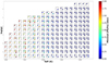 |
Fig. 2 Kiel diagram colour-coded with the lowest lead abundance (in dex) that could be detected in a spectrum whose (normalised) Pb line core flux is 0.5% deeper than that of a reference spectrum with [Pb/Fe] = −2.0 dex (i.e. negligible amount of Pb, and therefore undetectable line). For each combination of effective temperature and surface gravity, we estimated this lowest Pb abundance for three values of [M/H]: 0.0, −0.5, and −1.0 dex (from top to bottom and left to right in each small square). |
2.4 Lead abundance for stars with parameters outside the reference grid
During the analysis, about 20 spectra with atmospheric parameters and/or Pb abundances outside the 5D grid borders were identified ([Pb/Fe] > 2.0 dex and/or [Fe/H] < −2.5 dex). For analysing these specific cases with extreme parameters, we derive their lead abundances in a classical way, without using GAUGUIN. For that purpose, we computed synthetic spectra with the same tools as described above. MARCS models were interpolated at the AMBRE atmospheric parameters and synthetic spectra were computed with various lead abundances to found the best agreement between the normalised observed (provided by GAUGUIN) and simulated spectra. This procedure was checked and validated with some stars whose atmospheric parameters are within the grid and for which Pb abundances derived with GAUGUIN were available. Both Pb abundance estimates were found to be in perfect agreement, allowing to include these extreme parameter stars within the final catalogue of lead abundances, described below.
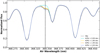 |
Fig. 3 Comparison between the solar observed spectrum from Wallace et al. (2011) (black dotted line) and a synthetic spectrum (interpolated to the Sun’s atmospheric parameters from Contursi et al. 2021) for different values of A(Pb) = 0.00, 1.80, 1.90, and 2.00. |
3 The AMBRE lead abundances catalogue
We present in this section the different steps that have been adopted to construct the AMBRE catalogue of lead abundances (i.e. the selection of the best derived values), the treatment of the repeats (as several spectra are available for some specific stars), the derivation of the uncertainties and the validation by comparison with literature values.
3.1 Solar lead abundance
Our automatic procedure leads to the fit between the solar observed and synthetic spectra (after calibration of the line list) shown in Fig. 3. We recall that the synthetic grid has been computed without calibrating the lead line atomic data and assuming the solar chemical abundances of Grevesse et al. (2007): A(Pb)6=2.00 dex. We also recall that we analysed the solar spectra of Wallace et al. (2011) degraded at R = 40000. Our derived solar LTE abundance is [Pb/Fe] = −0.20 dex, hence, A(Pb) = 1.80. The associated uncertainty is around ±0.01 dex.
This abundance is fully compatible with several previously published solar Pb photospheric values that analysed the same Pb line as we used: (Anders & Grevesse 1989, 1D model: A(Pb)=1.85), (Asplund et al. 2009, 3D model: A(Pb)=1.75), (Grevesse et al. 2015, 3D LTE models: A(Pb)=1.80). Nevertheless, we note that solar photospheric abundances are often smaller than meteoritic values obtained from CI carbonaceous chondrites (Lodders et al. 2009) with differences reaching about 0.25 dex. The rather complex spectral region upon which the lead line stands could explain the observed mismatches in the abundances, such as other physical assumptions as the selected atmospheric models and/or 1D/3D structure, LTE/NLTE effects. For instance, Mashonkina et al. (2012) estimated a NLTE correction of up to 0.20 dex for the Sun when adopting the same Pb line as we used.
As a conclusion, our automatic procedure derives a solar photospheric lead abundance that is fully consistent with literature values within less than ~0.05 dex, depending on the adopted physical assumptions. Therefore, no need of any calibration of our Pb abundance was found necessary.
3.2 Selection of the best analysed spectra
In some cases, GAUGUIN was unable to determine reliable lead abundances because of too low S/N spectra, too weak lead lines, cosmic rays and/or limitations in the parameters of some specific spectra with respect to the reference grid borders (see Sec. 2.4). Moreover, a weak lead line can be undetectable in high rotating stars, for which line blending could be extreme in the spectra.
In the following, we thus only considered slow-rotating stars when building the catalogue by filtering with the FWHMCCF parameter (Full Width at Half Maximum of the Cross-Correlation Function). This quantity is determined during the AMBRE parametrisation when estimating the radial velocity (VRad). It takes into account several broadening effects such as rotation and macroturbulent velocities. We therefore selected spectra with FWHMCCF < 15 km s−1, following previous AMBRE recommendations (Guiglion et al. 2016; Perdigon et al. 2021). This cut removes 13.4% and 18.4% spectra of the initial sample of UVES (considering the two setups) and FEROS, respectively (i.e. a total of 1467 spectra are then rejected because of their too large line-broadening).
On the other hand, we have systematically rejected any spectra whose abundance value is lower than 2.3 times the abundance upper limit for giants, defined as log(g) ≤ 3.5, and 2.8 times for dwarfs with log(g) > 3.5, (see Fig. 2). To select those thresholds, we looked at several observed spectra of various spectral types and visually chose the value above which the line cannot be mistaken with noise. In addition, we note that this upper limit also corresponds to the lowest Pb abundance that could be determined for a set of atmospheric parameters and a given S/N, as already discussed in Sec. 2.3. These rejection criterion were adopted in order to select only stars with the best detected Pb-line, compared to a spectrum without any Pb line detection (abundance upper limit). Since the Pb abundance measurement is fully automatic, some low-quality and/or too faint Pb-line spectra that could have suspicious Pb abundances are then automatically rejected. Such a procedure could reject good measurements for low lead abundance stars, but it guarantees a high-quality and a clean final sample of Pb abundances. A similar procedure was adopted for the chemical analysis of the Gaia/RVS spectra (see Recio-Blanco et al. 2023, for more details). Such a strict rejection of the faintest Pb signatures led to a final selection of 1341 stellar spectra (15.4% of the initial sample).
3.3 Uncertainties of the derived lead abundances
Various sources of uncertainties could impact our abundance determination and their respective importance is evaluated hereafter.
First, we quantified the impact of the flux noise on the abundance determination. Using the method described in Sec. 2, we actually reanalysed each observed spectrum a very large number of times with GAUGUIN, by estimating 1000 Monte-Carlo realisations of each spectrum, considering its flux uncertainties. Practically, this means that we built 1000 different versions of every observed spectra by noising their flux, considering their S/N ratio. Then, these 1000 noised realisations were automatically and independently analysed, leading to 1000 Pb abundances for a given star. This procedure then allowed to easily estimate the Pb abundance uncertainty caused by the flux uncertainty. Hereafter, the published A(Pb) corresponds to the median (50th quantile) of the 1000 Pb abundance distribution (hereafter denoted Q50). The associated upper and lower confidence values are estimated from the 84th and 16th quantiles (hereafter Q84 and Q16, respectively). Therefore, the Pb abundance dispersion defined by σMC=(Q84 − Q16)/2 is our adopted abundance uncertainty caused by the spectra S/N. This σMC means that there is a probability of 68% that the lead abundance is found within it. For each star, we note that we provide in the AMBRE catalogue Q84 and Q16 separately since the error bars are not always symmetric. To our knowledge, this is the first time that such a large number of spectra is chemically analysed so many times to derive one of their abundance and an extremely accurate estimate of its associated error caused by the flux uncertainties. We finally point out that σMC also takes into account some possible internal errors of the whole procedure as continuum normalisation, spectra quality, radial velocity correction.
It is found that, among the 1341 spectra selected in Sec. 3.2, 4% and 0.2% of them have a σMC larger than 0.10 and 0.20 dex, respectively. We report in Table 2 the mean estimated uncertainties of [Pb/Fe] for three main stellar types (cool giant, cool dwarf and solar-type) and for two values of S/N (65 and 110). The presented mean values are computed from all the AMBRE spectra which parameters are within a range of ± 150 K around the adopted central temperature and ± 15 around the indicated S/N. The number of stars (NS) used for the computation of the presented quantities is also indicated. As expected, σMC decreases with increasing S/N, leading to small dispersions for high S/N spectra (≲0.05 dex).
Then, we estimated the lead abundance A(Pb) sensitivity to typical uncertainties of the atmospheric parameters determined by the AMBRE Project, by reanalysing every spectrum adopting modified sets of atmospheric parameters. They are presented in Table 3 separately for a Teff, log(g), [M/H] uncertainty of ± 120 K, 0.25 and 0.10 dex, respectively, which are the mean values reported in the AMBRE parameter tables. We also report their quadratic sum (hereafter denoted ΔAtm) for the same three stellar types as in Table 2. We emphasise that this ΔAtm has been computed for each spectrum and is then reported for each star in the AMBRE catalogue. From Table 3 we note that [Pb/Fe] is more sensitive to temperature uncertainty, especially for cool giants. Even though the lines are more visible in their spectra, the continuum level placement is strongly impacted by the presence of numerous atomic and molecular features and could lead to less well defined line depths.
We note that errors of Vmicro ± 1 km s−1 and [α/Fe] ± 0.10 dex have no significant effect on the abundance value. This last point can be explained by the absence of lines from α-elements such as TiO in the studied spectral domain. We also point out that the above estimated errors obtained by varying Teff and log(g) also include macroturbulent velocity changes as this parameter value is modified according to the relation adopted in this work.
Uncertainties of the lead abundances A(Pb) caused by the spectra S/N for different stellar types.
Uncertainty of the A(Pb) lead abundances produced by typical uncertainties on the stellar atmospheric parameters for high-quality spectra (S/N>100).
3.4 Final AMBRE:Pb catalogue
As already discussed, our sample is composed of a large number of stars for which several spectra are available. Similarly to the procedure adopted in Santos-Peral et al. (2020) and Perdigon et al. (2021), we performed a cross-match between the Gaia e-DR3 ID (Gaia Collaboration 2021) and the AMBRE catalogue. For a couple of stars, no Gaia ID were found and we therefore adopted their HD name.
Among the 1341 spectra having passed the selection criteria presented in Sec. 3.2 (e.g. removing highly rotating stars, too low S/N, no detected lines), we found that they correspond to 653 different stars, 32.1% of them being giants. 72.4% of the total sample stars have only one spectrum whereas 3.5 % of them have more than ten repeats. The metallicity range of this sample star varies from approximately −2.9 dex to +0.6 dex with lead abundances varying from −0.7 dex to 3.3 dex. For each star, we checked that the repeat spectra (if some are identified) were parametrised in a very consistent way among each other. We indeed systematically rejected individual spectra of a given star whose parameters are found outside the standard deviation in Teff, log(g) and [M/H], calculated for all the available repeats. The adopted threshold were 110 K, 0.5 and 0.20 dex, respectively.
We report this AMBRE catalogue of lead abundances in Table 4. With about 650 stars, this is the largest catalogue ever published (as can be seen from Figs. 16 and 32 of Prantzos et al. (2018); Kobayashi et al. (2020), respectively). For each star, we report their number Nspec of available repeat spectra if any (only spectra who passed the selection criteria), the star ID (Gaia DR3 or HD name) and their Teff, log(g), [M/H], [α/Fe] (or mean values if repeats are available). The lead abundances are provided by the median of the LTE A(Pb) Monte-Carlo distributions (Q50 values, or their mean in case of repeats), together with their associated Q84 and Q16. The quadratic sum of errors caused by atmospheric parameters uncertainties (ΔAtm) as described in Sect 3.3, is also provided.
We then took into account all the uncertainty sources estimated above by computing the quadratic sum of ΔAtm (caused by the atmospheric parameter uncertainties) and σMC (caused by the spectra S/N). We found a mean uncertainty (ΔPb) of about 0.10 dex with a standard deviation of 0.04 dex, for all the AMBRE:Pb catalogue stars. This uncertainty ΔPb is published for any star in Table 4. We also found that the mean Pb abundance dispersion for stars having more than one repeat is about 0.04 dex. We can therefore conclude that the reported lead abundances present a very good consistency and measurement precision between each other.
Finally, we also report in Table 4 the corresponding NLTE Pb abundances. They were estimated by adding to our LTE lead abundance the NLTE corrections calculated by Mashonkina et al. (2012, and private communication for the NLTE corrections specific to the selected Pb I 368.3 nm line). The applied NLTE corrections were interpolated in the provided table at the parameters of our stars. They are of the order of ~+0.15 dex for dwarf stars and about twice larger for giants. They satisfactory correct the systematic differences observed between the LTE Pb abundances of these two types of stars.
To illustrate this AMBRE:Pb catalogue, we show in Fig. 4 the Kiel diagram of our 653 stars colour-coded by their metallicity (left panel) and their NLTE Pb abundance (right panel). We can see again that the majority of our sample is dominated by dwarf stars. Rather few stars seem to be on the Asymptotic Giant Branch and a few others are metal-poor and lead-enhanced. They are discussed in Sects. 4.1 and 4.2, respectively.
AMBRE catalogue of lead abundances.
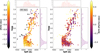 |
Fig. 4 Kiel diagrams of the 653 AMBRE:Pb stars, colour-coded by their metallicity (left panel) and their NLTE Pb abundance (right panel). |
3.5 Validation thanks to literature comparisons
Among the 653 stars present in our AMBRE:Pb catalogue, eleven have LTE Pb abundances already published in the literature. Figure 5 shows the comparison between these AMBRE:Pb abundances and those of the literature colour-coded by the differences in Teff (top panel) and log(g) (central panel) and [M/H] (lower panel) in the sense (Literature – AMBRE).
Globally, we first remark that the AMBRE:Pb abundances are compatible with the literature, as are their adopted atmospheric parameters. The median of the differences in Pb is around −0.2 dex with a dispersion of 0.26 dex, which corresponds to the typical dispersions between the different literature values, considering their uncertainties. Only for two peculiar stars the differences are larger. First, our Pb abundance for HE 0338-3945 (Gaia DR3 4856059422664301440, a very metal poor star with [M/H]= −2.09 dex) is larger than that of Jonsell et al. (2006) and Hampel et al. (2019) by 0.50 dex and 0.86, respectively. These differences in the Pb abundances can be explained by the different values of log(g) and [M/H] adopted by the different studies. The AMBRE log(g) is indeed about 0.4 higher than that of Jonsell et al. (2006) and Hampel et al. (2019). But, more importantly, differences in metallicity of about 0.6 dex are found between AMBRE and these two other works. Second, for CS 22947-187 (Gaia DR3 6663163201607650688, [M/H] = −2.92 dex), our Pb abundance is 0.80 dex higher than that of Roederer et al. (2014), even though their atmospheric parameters are fully compatible with ours. We have carefully re-examined and re-analysed this AMBRE spectra and the low abundance reported by Roederer et al. (2014) is not compatible with our data.
Finally, we have also compared our adopted AMBRE stellar atmospheric parameters with those recently published by the Gaia/DPAC GSP-spec module, in charge of the analysis of the Gaia Radial Velocity Spectrometer data (Recio-Blanco et al. 2023). After having applied a very strict filtering based on the quality flags recommended by these authors, 417 stars are found in common between AMBRE and GSP-spec. The median of the Teff, log(g), [M/H] differences7 are found to be rather small and equal to 86 K, −0.03 dex and 0.03 dex, respectively, whereas their Median Absolute Deviation is 186K, 0.18 and 0.10 dex. The AMBRE and GSP-spec have therefore published very consistent stellar atmospheric parameters.
In conclusion, the AMBRE:Pb catalogue provides high-quality stellar parameters and lead abundances. It allows to explore the lead chemical properties in different type of stars (Sec. 4) together with the evolution of this species in the Milky Way (Sec. 5).
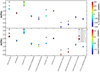 |
Fig. 5 AMBRE LTE A(Pb) abundances (filled stars) and the literature values (see legend in inset): wide diamonds are from Travaglio et al. (2001), pentagon from Van Eck et al. (2001), up pointing triangle from Sivarani et al. (2004), hexagon from Ivans et al. (2005), down pointing triangle from Jonsell et al. (2006), plus sign from Roederer (2012), squares from Hampel et al. (2019), narrow diamonds from Roederer et al. (2010), and circles from Roederer et al. (2014). The top and bottom panels are colour-coded by the difference between the literature and AMBRE Teff values and the literature and log(g) values, respectively. |
4 Lead abundance in peculiar stars
The AMBRE:Pb catalogue contains a total of 653 stars. Most of them are main-sequence (429 stars, i.e. 66%, defined by log(g)>3.5) and red giant stars (204 stars, 31%) with metallicities greater than −1.0 dex. 20 stars (of any gravity) are found to be more metal-poor than this value and 15 dwarf are more metalrich than 0.3 dex. In this catalogue, one also finds three AGB stars, nine lead-enhanced metal-poor stars and 13 Gaia Benchmark Stars. Their content in lead is described in the following subsections.
4.1 Asymptotic Giant Branch stars
In the AMBRE:Pb catalogue, three stars (HD 29139, Gaia DR3 5306951892625773312, and Gaia DR3 6083708032481982336) have atmospheric parameters suggesting that they could be located on the Asymptotic Giant Branch (AGB, Teff < 4000 K and log(g) <2.0). These stars are found to be not enriched in Pb, their [Pb/Fe] being close to 0 dex. Therefore, they are probably in the early AGB phase and have not yet experienced third dredge-up events that should have enriched their atmosphere in Pb. This is consistent with their rather hot Teff (larger than 3700 K) and rather high surface gravity found between 1.1 and 1.5, with respect to more evolved AGB. We finally recall that, during the AMBRE parametrisation, we assumed that these AGB are not carbon-rich, which is also consistent with their no lead enrichment nature.
4.2 Lead enhanced metal-poor stars
In the AMBRE:Pb catalogue, nine metal-poor stars8 are found to be strongly enhanced in lead, with [Pb/Fe]>1.5 dex, without considering NLTE corrections. Among them, only two have already been identified in the literature as lead-enhanced stars, and therefore, seven are new discoveries:
First, our A(Pb) abundance of Gaia DR3 4856059422664301440 (also known as HE 0338-3945) confirms its Pb-enhanced nature previously reported by Jonsell et al. (2006) and Hampel et al. (2019). However, as already discussed in the previous section, these three reported Pb abundances differ slightly because of differences in the adopted atmospheric parameters. Moreover, this star has been identified as a Carbon-enhanced metal-poor star (CEMP) of s-II type ([Ba/Eu] > 0.5 dex and [Eu/Fe] > 1.0 dex) according to Barklem et al. (2005). Such enhancements have also been confirmed by Abate et al. (2015).
Similar conclusions can be drawn for Gaia DR3 6907236881547590144 (HD 196944) whose Pb abundance was also previously derived by Van Eck et al. (2001). This star seems also to be a CEMP star classified as CEMP -s/rs according to Yoon et al. (2016) or CEMP-s according to Karinkuzhi et al. (2021). Such carbon and s-process element enhancement have also been highlighted in Zacs et al. (1998).
For the seven newly discovered Pb-enriched stars reported in the present work, we note that Gaia DR3 6663163201607650688, 2347402354016302208, 2604742840043317760, 2604742840043317760, 3790607572739648000 and 2601354871056014336 were also already identified as CEMP stars with s-process enrichments (Aoki et al. 2002; Komiya et al. 2007; Abate et al. 2015; Yoon et al. 2016). However, no chemical information have been found for Gaia DR3 6299901567857374848, that could be a new CEMP star candidate. Its parameters are Teff=4680 K, log(g)=1.4, [M/H]=-2.6 dex and [Pb/Fe]=1.58 dex.
It is interesting to note that, thanks to Gaia DR3 astrometric information, the binary nature of these stars can be explored. We have indeed check their ruwe and duplicated_source parameters, their ipd_frac_multi_peak and non_single_star parameters showing no peculiar value. Among the nine stars described above, five are suspected binaries that could help to interpret their nature. Gaia DR3 2347402354016302208, 2604742840043317760, 3790607572739648000 and 6907236881547590144 have their ruwe parameters well larger than 1.4. Moreover, Gaia DR3 6663163201607650688 has its duplicated_source equal to True. Therefore, following Gaia, these five stars of the sample of Pb-enriched metal-poor stars could therefore belong to a binary system whereas the remaining four do not have any clues of a possible multiple star nature. This should be confirmed with the future Gaia data releases that will span a much larger timescale than the DR3, helping to better detect any possible binary signature.
Several scenarios could be invoked to produce such Pb enriched stars and, more generally, s-process elements enrichments. The main one for CEMP-s stars is a binary-mass transfer between an AGB star that has produced carbon and heavy elements and a less evolved companion (e.g. Abate et al. 2015). It is highly probable that our candidates belong to this category. However, some stars are both s- and r-process enriched and could thus not be formed only thanks to AGB winds. Even if not all the processes are understood, many scenarios have been investigated to explain such exotic abundance patterns. Among them, one could first cite a binary system formed in a molecular cloud already enriched in r-process elements by the nearby explosion of one or more Type II supernovae (e.g. Jonsell et al. 2006; Bisterzo et al. 2012; Sneden et al. 2014). Another scenario assumes that one of the member of a binary system is relatively massive and undergoes the AGB phase, producing s-elements, but then explodes as an electron-capture supernova, providing the r-elements (e.g. Jonsell et al. 2006). Finally, many works have suggested that both r- and s-elements could be synthesised in low-mass, extremely metal poor AGB stars ([Fe/H]<−3 dex): these stars might generate high densities of free neutrons during the ingestion of protons in the region of the He-flash (e.g. Cristallo et al. 2009a; Lugaro et al. 2009; Cristallo et al. 2016; Choplin et al. 2021, 2022).
Lead abundances in Gaia Benchmark Stars adopting the Jofré et al. (2018) atmospheric parameters.
4.3 Lead abundance in Gaia Benchmark Stars
Finally, Table 4 also contains lead abundances, adopting the AMBRE atmospheric parameter values, for 13 Gaia benchmark stars, hereafter denoted GBS (see Jofré et al. 2018, and references therein). These FGKM-type stars are commonly adopted to calibrate and/or validate large spectroscopic surveys as their atmospheric parameters were carefully derived using several techniques.
For some of them, these parameters could slightly differ from the derived AMBRE ones since the analysis technics and observed data differ. For consistency with already published values, we recomputed their lead abundance adopting the atmospheric parameters of Jofré et al. (2018). The results are presented in Table 5, which is structured similarly as Table 4, (excepted for the ΔAtm column). We note that the adopted [α/Fe] is the mean of the individual Mg, Si, Ca and Ti abundances from Jofré et al. (2018). We also added the solar and Arcturus abundances already shown in Table 5 computed from Wallace et al. (2011) and Allende Prieto et al. (2004) spectra, respectively. Except for HD120283, for which we found a [Pb/Fe] difference of 0.15 dex with respect to Table 4, caused by a Teff difference of about 220 K, we remark that these new [Pb/Fe] abundances reported in Table 5 differ by only 0.05 dex (in median) with respect to the AMBRE:Pb values. Such tiny differences are completely explained by the small differences on the adopted atmospheric parameters.
5 The Milky Way lead abundance
5.1 Spatial and kinematic distributions
In this section, we first investigate the spatial and kinematical distribution of the AMBRE:Pb Catalogue. For that purpose, we computed the stellar positions (Galactocentric Cartesian coordinates X, Y, Z) as well as the Galactocentric radius (R) and cylindrical velocities (VR, VZ and Vϕ) as presented in Gaia Collaboration (2023), using the Gaia eDR3 photogeometric distances from Bailer-Jones et al. (2021). We note that these quantities were computed for the 485 AMBRE:Pb stars having Gaia DR3 data, especially distances (74% of the whole sample). The top panels of Fig. 6 show this sample in the (X, Y) plane, whereas the bottom panels correspond to the (R, Z) plane. The left panels are colour-coded by the stellar counts and the right panels by Vϕ. It can be seen that the majority of the stars (92.7%) are located in a box of 1 kpc size around the solar position, confirming the solar neighbourhood nature of the AMBRE:Pb sample. This is confirmed by the right panels of Fig. 6 where 91% of the stars are found close to the Galactic Plane (|Z| < 0.7 kpc).
Moreover, Fig. 7 show the Toomre diagram of these 485 stars. 70% of the stars have a total velocity smaller than 70 km s−1, an indication that they may belong to the disc component of the Milky Way. However, some metal-poor stars present a total velocity larger than 150 km s−1 and may probably belong to the Galactic halo.
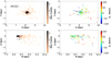 |
Fig. 6 Galactic distributions of the AMBRE:Pb catalogue stars. The top panels show the distributions in Cartesian coordinates (X, Y), colour-coded by stellar counts (left panel) and (right panel). The bottom panels show the (R, Z) distributions with the same colour-coding as the top panels. The very few most distant stars are not seen in these plots. |
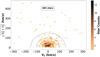 |
Fig. 7 Toomre diagram of the AMBRE:Pb stars colour-coded by their number. |
5.2 Lead in the Milky Way disc
We then investigate the chemical trend of lead abundances in the Milky Way disc. To do this, we selected only stars with a total velocity smaller than 75 km s−1, |Z| < 0.70 kpc and an uncertainty on Pb abundances smaller than 0.10 dex. We also rejected the above discussed nine Pb-enriched metal-poor stars since their atmosphere is not representative of the ISM chemical composition from which they formed. This selection leads to a sample of 265 bona – fide high-quality disc stars. From the selected sample, we computed the Pb radial and vertical gradients of the Galactic disc, thanks to Theil-Sen fits to the data as already performed in Contursi et al. (2023). Uncertainties were computed by adopting a confidence level of 0.95. We note that, contrarily to previous AMBRE studies (see, for instance, Perdigon et al. 2021; Santos-Peral et al. 2021), we did not separate the thin and thick components of the disc because of too low statistics.
Regarding the [Pb/Fe] radial gradient over a range of R between 8 to 9.5 kpc, we found δ[Pb/Fe]/δR = 0.012±0.046 dex kpc−1. This value if fully compatible within error bars with the cerium9 radial gradient computed both in Contursi et al. (2023) and with the value provided by Tautvaišienė et al. (2021). We also found δ[Pb/H]/δR = 0.005±0.017 dex kpc−1, which is again compatible with the δ[Ce/H]/δR derived in Contursi et al. (2023), as well as [Ce/H] and [La/H] radial gradients from Cepheids derived in da Silva et al. (2016) over a wider range of Galactocentric distances (4–18 kpc).
Then, we estimated the vertical gradients for the Pb abundances for Z-values varying from −0.65 to +0.21 kpc. A positive (but not significative within error bars) trend was found with δ[Pb/Fe]/δZ = 0.036±0.037 dex kpc−1, similarly to the Ce abundances trend derived by Contursi et al. (2023). Similarly, we also derived δ[Pb/H]/δZ = 0.010±0.014 dex kpc−1.
5.3 Comparison between the lead, europium, barium and α-trends
We now investigate the respective behaviours of the Pb, Eu, Ba and α abundance trends as a function of metallicity in the Milky Way disc (see Fig. 8). The [Pb/α], [Pb/Ba] and [Pb/Eu] ratios were estimated by adopting the lead abundances derived in the present study, the α-abundances derived within the AMBRE Project during the stellar parametrisation process (Worley et al. 2012, 2016), and the AMBRE europium and barium abundances from Guiglion et al. (2018). For that purpose, we searched which of our 265 Galactic disc stars with high-quality Pb abundances are also found in the Eu and Ba samples, considering only stars with an error in [Eu/Fe] and [Ba/Fe] smaller than 0.10 dex. We end up with 93 and 127 stars with both Pb plus Eu and Ba, respectively. Their metallicities is found in the range between ~-0.8 to ~0.3 dex.
In Fig. 8, we show the different ratios derived for each star (blue points) together with a running mean, adopting bins of 0.1 dex in metallicity (orange points)10. It can first be seen that [Pb/M] well decreases with the metallicity, reaching [Pb/M] values close to 0 at solar metallicity. The decrease seems to be also present for super-solar metallicities. Such a decrease is significant, considering the dispersions associated to the running mean (vertical lines for each orange dot). On the other hand, the [Pb/Eu] ratio seems to be slightly decreasing as metallicity increases. However, the large dispersions associated to these data are fully compatible with a flat trend around the zero-value. On the contrary, flat trends for [Pb/α] and [Pb/Ba], close to 0.0 dex, are shown in the bottom panels, although the dispersions are again rather large. These trends are interpreted below thanks to Galactic chemical evolution models.
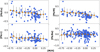 |
Fig. 8 Behaviour of Pb over Eu, mean metallicity, and α and Ba abundances vs. metallicity. The blue points refer to the analysed stars, whereas the orange points are the abundance ratio mean by 0.1 dex metallicity bins (except for the most metal-rich bin which is 0.25 dex). The associated dispersions in each bin is also indicated (vertical black lines). |
5.4 The Galactic chemical evolution of lead
The chemical properties of the 265 Galactic disc stars with high-quality Pb abundances are compared to Galactic chemical evolution models, in order to better understand the chemical evolution of lead. This is illustrated in Fig. 9 where the observed Pb abundance patterns in the [Pb/Fe] versus [M/H] plane are compared to different chemical evolution models. The chemical evolution models differ between themselves mainly by the number of infall episodes. In particular, the shown models are as follows:
the one-infall model (see e.g. Matteucci & Francois 1989; Grisoni et al. 2018), which assumes that the solar neighbourhood is formed by means of a single infall of primordial gas with a timescale of τ ≃ 7 Gyr.
the two-infall model of Spitoni et al. (2021) (see also Spitoni et al. 2019) assuming that the Milky Way disc formed as a result of two distinct gas accretion episodes. The first one formed the chemically defined thick disc (namely the high-α sequence) whereas the second one, delayed by ~4 Gyr, is responsible for the formation of the thin disc one (namely the low-α sequence). The first gas infall is characterised by a much shorter accretion timescale (τ1 ≃ 0.1 Gyr) than the second one (τ2 ≃ 4.0 Gyr). The original model adopted the set of yields of François et al. (2004) for massive stars. Here, we adopt yields derived from Limongi & Chieffi (2018)’s sets, as described below.
the three-infall model of Spitoni et al. (2023) which is an extension of the two-infall one of Spitoni et al. (2021). It was designed to reproduce the low-α sequence by means of two distinct gas infall episodes (the most recent one which started ~2.7 Gyr ago) in order to reproduce the young chemical impoverishment in metallicity with low [α/Fe] values first revealed by the Gaia Collaboration (2023), as well as the recent enhanced star formation activity of Ruiz-Lara et al. (2020).
Prescriptions for the adopted star formation (here parametrised as proportional to the Schmidt–Kennicutt law (Kennicutt 1998) and initial mass function (Kroupa et al. 1993) are the same for the different models. Moreover, all of them are able to well reproduce the Type Ia SNe, Type II SNe and merging neutron star (MNS) rates as observed by Cappellaro et al. (1999) (for SNe) and Kalogera et al. (2004) (for MNS).
With regard to the nucleosynthesis prescriptions, we recall that Pb is formed both through s- and r-process channels (~83% and −17% at solar metallicity, respectively according to Prantzos et al. 2020). In this work, we adopt a similar nucleosynthesis to that used by Molero et al. (2023), and we refer to this work for a detailed discussion. In summary, we assume that the r-process nucleosynthesis takes place in (i) MNS, with yields scaled to those of Sr from the kilonova AT2017gfo (Watson et al. 2019) and in (ii) magneto-rotational supernovae (MR-SNe), with yields from Nishimura et al. (2017)’s model L0.75. MNS are assumed to merge with a delay time distribution (DTD) function and MR-SNe are assumed to be 20% of massive stars with initial mass between 10 − 25 M⊙. The s-process nucleosynthesis is assumed to happen in (i) low- and intermediate-mass stars (LIMS; M ≤ 8 M⊙) during their AGB phase with yields prescriptions from the FRUITY database (Cristallo et al. 2009b, 2011, 2015), and in (ii) rotating massive stars (M ≥ 13 M⊙), with yields from Limongi & Chieffi (2018)’s recommended set R. Details regarding the model prescriptions are reported in Table 6. As discussed in Sec. 1, the main stellar nucleosynthesis sites of Pb are, in particular, low-mass low-metallicity AGB stars. The non-rotational set of the FRUITY database provides accurate yield grids for 96 stellar progenitors with initial masses and metallicities spanning the ranges 1.3–6.0 M⊙ and 2 × 10⁻⁵ −2 × 10⁻², respectively. Although the great precision provided by a large number of progenitors, the current set of FRUITY yields tends to overestimate the s-process contribution for most neutron-capture elements. This feature has already emerged in previous chemical evolution studies (e.g. Rizzuti et al. 2019; Magrini et al. 2021; Rizzuti et al. 2021; Molero et al. 2024). The need to reduce the AGB yields appears evident in the case of Pb as well, independently from prescriptions regarding massive stars. This is shown in the upper left panel of Fig. 9, where Model 1, with no reduction in the AGB yields, creates a bump at intermediate metallicities (−0.9 ≤ [M/H] ≤ −0.1 dex) dex which overproduces the observed trend.
As a “Gedanken Experiment” we run a GCE model in which the evolution of the AGB models has been frozen as soon as they attain C/O=1 on their surfaces. As a consequence, s-process yields result decreased, being this effect more evident at lower metallicities, where the C-rich regime is reached in the first part of the AGB track. Fig. 9 demonstrates that our working hypothesis, despite being extreme, works in the right direction (Model 2), possibly highlighting that the adopted mass-loss rate in FRUITY models is underestimated. Currently, AGB mass-loss rate in FRUITY models is evaluated basing on observational period – mass-loss data (see Straniero et al. 2006 for details). However, the period is theoretically estimated basing on period-luminosity relations in which a distinction between O-rich and C-rich stars has not been operated (e.g. Feast et al. 1989). More recent works pointed out that those relations may vary with the C/O ratio, leading to larger mass-loss rates in the C-rich regime (Groenewegen et al. 2020; Ita et al. 2021). We postpone to a future work a detailed analysis on this topic. Here, we simply conclude that a reduced production of Pb from AGB stars noticeably improves the agreement with the observations.
For rotating massive stars, differently from Molero et al. (2023), two more sets have been considered, corresponding to two different theoretical distributions for the velocities. Similarly to Romano et al. (2019) (see also Rizzuti et al. 2021), we assume that the probability that a star rotates faster increases with decreasing metallicity. In this way, we should be able to provide a better fit to the few data observed at [M/H] ≤ −0.1 dex. We recall that the assumption of having a distribution of rotational velocity rather than a fixed one is more physical and supported both theoretically (Frischknecht et al. 2016) and observationally (Martayan et al. 2007; Hunter et al. 2008; Chiappini et al. 2011; Prantzos et al. 2018). The two new distributions, DIS1 and DIS2, assume that stars have an initial rotational velocity of 300 and of 175 km s−1, respectively, for Z ≤ 3.236 × 10⁻³ and of 150 km s−1 for higher values of Z (Model 3 and Model 4, respectively). As expected, rotation in massive stars increases the production of Pb, causing Model 3 to overestimate the [Pb/Fe] versus [M/H] trend. Only Model 4, with a mild increase in the rotational velocities at low Z, is able to provide an adequate fit with the observations.
Deviations between the Model 4 predictions and the observed trend are present for metallicities above solar for the one-infall model. An agreement in this range of metallicities is partially obtained with a scenario of disc formation including more than one infall (Model 5 and Model 6), in particular in the case of the two-infall model from Spitoni et al. (2021), because of the shorter first infall timescales (see lower panels of Fig. 9). To strengthen our assumptions on the nucleosynthesis, in particular of AGB and massive stars, here we show that our model correctly reproduces the abundance patterns of the second peak s-process element Ba. In Fig. 10, we present results for the one-infall and two-infall (from Spitoni et al. 2021) models compared to the observed average trends of the [Pb/Ba] and [Ba/Fe] versus [M/H]. We recall that the models shown in the figure differ only by the initial rotational velocities of massive stars (see Table 6). The models are in excellent agreement with the observed trend, in particular for [M/H]≤ −0.s dex and in the case of the [Ba/Fe] versus [M/H]. The [Pb/Ba] ratio is slightly overproduced in the low-metallicity regime by all models, even if the predictions fall well in the uncertainty ranges.
In Fig. 11, we report results for the one-infall and two-infall (from Spitoni et al. 2021) models compared to the observed average trends of the [Pb/Eu], [Pb/α], [Eu/α], and [Eu/Fe] versus [M/H] presented in the previous section. We decided to use oxygen as a comparison for the α, since it is actually mainly produced by Type II SNe with low pollution from Type Ia SNe, which makes the comparison easier. All the models are able to provide a good fit with the observed data. The flat trend discussed in Saction 5.3 is well reproduced and differences between the models for the [Pb/Eu] and the [Pb/α] trends are visible only at low [M/H]. The slight decrease observed in the [Pb/Eu-α] as well as the rise of the [Eu/α] towards higher [M/H] is also visible in the model predictions, which provide an overall nice agreement with the observations. At low metallicities, the model which best reproduces the observed patterns is the one with higher rotational velocity at low Z (Model 3, corresponding to 300 km s−1) which, as already discussed, increases the production of Pb. It should be noted that higher rotational velocity of massive stars does not affect the production of Eu and of α. In fact, in our models Eu is not produced by normal core-collapse SNe. On the other hand, the production of α is increased for rotational velocities higher than 0 km s−1, but above 150 km s−1 there are no significant differences (see Romano et al. 2019 for details).
In summary, the model which better fits the observed [Pb/Fe] versus [M/H] abundance pattern is the two-infall model from Spitoni et al. (2021), with a distribution of initial rotational velocities of massive stars which favours higher velocities towards lower metallicities. Yields of Pb from AGB stars should be lower than the original FRUITY models, at least for lower metallicities, similarly to what is artificially done for other s-process elements (see e.g. Rizzuti et al. 2019; Molero et al. 2023). The observed trends of the [Pb/Eu], [Pb/α], [Eu/α], and [Eu/Fe] versus [M/H] are also well reproduced by models that favour higher rotational velocities towards lower [M/H] values. In this case, adopting a one-infall or a two-infall model does not produce significant differences in the predictions.
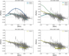 |
Fig. 9 Model predictions for the [Pb/Fe] vs. [Fe/H] abundance pattern. Upper panels: predictions for a single infall and for different contributions from AGB stars (Model 1 and Model 2) as well as different initial rotational velocities (IRV) of massive stars (Model 3 and Model 4). Lower panels: predictions for models with more than one infall, massive stars yields weighted with the DIS2 distribution of rotational velocities, and new yields from AGB stars (Model 5 and Model 6). For the models details we refer to Table 6. |
Nucleosynthesis prescriptions for the s-process and number of infalls for different models.
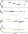 |
Fig. 10 Model predictions for the [Pb/Ba] and [Ba/Fe] abundance patterns for the one-infall model (upper panels) and the Spitoni et al. (2021) two-infall model (lower panels). |
6 Summary
We have presented the AMBRE:Pb catalogue that contains LTE and NLTE lead abundance of 653 stars. This is the largest catalogue of homogeneous lead abundances ever published. It relies on the automatic analysis of the Pb I 368.346 nm line of more than 8 million spectra, thanks to the GAUGUIN method. The stellar atmospheric parameters were adopted from the AMBRE parametrisation. Pb abundance uncertainties resulting from the S/N spectra were estimated by independently analysing 1000 flux spectra realisations. This catalogue has then been validated thanks to literature comparison.
Most of the AMBRE:Pb stars are dwarf with metallicities higher than ~-1.0 dex, up to ~+0.3 dex. Their spatial and kinematic properties confirm that most of them are located within ~1 kpc from the Sun, and probably belong to the Galactic disc. The [Pb/Fe] abundance ratio is found to slightly decrease with metallicity. Radial and vertical gradients of δ[Pb/Fe]/δR = 0.012±0.046 dex kpc−1 and δ[Pb/Fe]/δZ = 0.036±0.037 dex kpc−1 were estimated for disc stars. Moreover, for a sub-sample of these stars, α and europium abundances were previously derived within the AMBRE Project. Flat trends within uncertainties in [Pb/Eu] and [Pb/α] over the [−0.75, +0.25] metallicity regime are seen.
These behaviours have been interpreted thanks to Galactic evolution models. The observed trends are well reproduced by the two-infall model, considering either Pb, Eu and α-abundance ratios. However, a strong reduced contribution from AGB stars and higher rotational velocities for low-metallicity massive stars have to be invoked. In any case, below [M/H]~-1.0 dex, our data are statistically insufficient to well constrain the models that could predict larger ratios than observed.
In addition, some peculiar stars are also identified in the AMBRE:Pb catalogue. Three probable Asymptotic Giant Branch stars are found to be not enriched in lead, revealing that they still did not experience any third-dredge-up events. On the contrary, nine stars very enriched in lead are found, eight of them being known as Carbon-Enriched Metal-Poor (CEMP) stars. The last one could thus be a new CEMP candidate. Moreover, the Pb abundance of 13 Gaia Benchmark Stars are also reported, adopting both the AMBRE and the literature reference values for their atmospheric parameters.
This AMBRE:Pb catalogue is made publicly available and should be an important step forward in our understanding of the Galactic chemical evolution of very heavy neutron-captured elements and of their production rates in different types of stars.
Data availability
Full Table 4 is available at the CDS via anonymous ftp to cdsarc.cds.unistra.fr (130.79.128.5) or via https://cdsarc.cds.unistra.fr/viz-bin/cat/J/A+A/690/A97
Acknowledgements
The authors thank L. Mashonkina for providing the NLTE corrections for the Pb I 368.3 nm line. We also thank T. Masseron for having shared some molecular line lists partially used within the AMBRE Project. This work has made use of data from the European Space Agency (ESA) mission Gaia (https://www.cosmos.esa.int/gaia), processed by the Gaia Data Processing and Analysis Consortium (DPAC, https://www.cosmos.esa.int/web/gaia/dpac/consortium). Funding for the DPAC has been provided by national institutions, in particular the institutions participating in the Gaia Multilateral Agreement. This work has also made use of the VALD database, operated at Uppsala University, the Institute of Astronomy RAS in Moscow, and the University of Vienna. We also used the SIMBAD database, operated at CDS, Strasbourg, France. Part of the calculations were performed with the high-performance computing facility SIGAMM, hosted by OCA. This work was supported by the Deutsche Forschungsgemeinschaft (DFG, German Research Foundation) — Project-ID 279384907 – SFB 1245, the State of Hessen within the Research Cluster ELEMENTS (Project ID 500/10.006). Finally, we are grateful to the anonymous referee for their constructive feedback, which has improved the clarity of the manuscript.
References
- Abate, C., Pols, O. R., Izzard, R. G., & Karakas, A. I. 2015, A&A, 581, A22 [NASA ADS] [CrossRef] [EDP Sciences] [Google Scholar]
- Allen, D. M., & Barbuy, B. 2006, A&A, 454, 917 [NASA ADS] [CrossRef] [EDP Sciences] [Google Scholar]
- Allende Prieto, C., Barklem, P. S., Lambert, D. L., & Cunha, K. 2004, A&A, 420, 183 [NASA ADS] [CrossRef] [EDP Sciences] [Google Scholar]
- Anders, E., & Grevesse, N. 1989, Geochim. Cosmochim. Acta, 53, 197 [Google Scholar]
- Aoki, W., Ryan, S. G., Norris, J. E., et al. 2002, ApJ, 580, 1149 [Google Scholar]
- Arlandini, C., Käppeler, F., Wisshak, K., et al. 1999, ApJ, 525, 886 [Google Scholar]
- Asplund, M., Grevesse, N., Sauval, A. J., & Scott, P. 2009, ARA&A, 47, 481 [NASA ADS] [CrossRef] [Google Scholar]
- Asplund, M., Amarsi, A. M., & Grevesse, N. 2021, A&A, 653, A141 [NASA ADS] [CrossRef] [EDP Sciences] [Google Scholar]
- Bailer-Jones, C. A. L., Rybizki, J., Fouesneau, M., Demleitner, M., & Andrae, R. 2021, AJ, 161, 147 [Google Scholar]
- Barbuy, B., Spite, M., Hill, V., et al. 2011, A&A, 534, A60 [NASA ADS] [CrossRef] [EDP Sciences] [Google Scholar]
- Barklem, P. S., Christlieb, N., Beers, T. C., et al. 2005, A&A, 439, 129 [NASA ADS] [CrossRef] [EDP Sciences] [Google Scholar]
- Biémont, E., Garnir, H. P., Palmeri, P., Li, Z. S., & Svanberg, S. 2000, MNRAS, 312, 116 [CrossRef] [Google Scholar]
- Bijaoui, A. 2012, in Seventh Conference on Astronomical Data Analysis, eds. J.-L. Starck, & C. Surace, 2 [Google Scholar]
- Bisterzo, S., Gallino, R., Straniero, O., Cristallo, S., & Käppeler, F. 2012, MNRAS, 422, 849 [Google Scholar]
- Brooke, J. S. A., Bernath, P. F., Schmidt, T. W., & Bacskay, G. B. 2013, J. Quant. Spec. Radiat. Transf., 124, 11 [NASA ADS] [CrossRef] [Google Scholar]
- Burbidge, E. M., Burbidge, G. R., Fowler, W. A., & Hoyle, F. 1957, Rev. Mod. Phys., 29, 547 [NASA ADS] [CrossRef] [Google Scholar]
- Busso, M., Gallino, R., & Wasserburg, G. J. 1999, ARA&A, 37, 239 [Google Scholar]
- Busso, M., Gallino, R., Lambert, D. L., Travaglio, C., & Smith, V. V. 2001, ApJ, 557, 802 [CrossRef] [Google Scholar]
- Cappellaro, E., Evans, R., & Turatto, M. 1999, A&A, 351, 459 [NASA ADS] [Google Scholar]
- Chiappini, C., Frischknecht, U., Meynet, G., et al. 2011, Nature, 472, 454 [Google Scholar]
- Choplin, A., Siess, L., & Goriely, S. 2021, A&A, 648, A119 [NASA ADS] [CrossRef] [EDP Sciences] [Google Scholar]
- Choplin, A., Siess, L., & Goriely, S. 2022, A&A, 667, A155 [NASA ADS] [CrossRef] [EDP Sciences] [Google Scholar]
- Clayton, D. D., & Rassbach, M. E. 1967, ApJ, 148, 69 [Google Scholar]
- Contursi, G., de Laverny, P., Recio-Blanco, A., & Palicio, P. A. 2021, A&A, 654, A130 [NASA ADS] [CrossRef] [EDP Sciences] [Google Scholar]
- Contursi, G., de Laverny, P., Recio-Blanco, A., et al. 2023, A&A, 670, A106 [NASA ADS] [CrossRef] [EDP Sciences] [Google Scholar]
- Couch, R. G., Schmiedekamp, A. B., & Arnett, W. D. 1974, ApJ, 190, 95 [NASA ADS] [CrossRef] [Google Scholar]
- Cristallo, S., Piersanti, L., Straniero, O., et al. 2009a, PASA, 26, 139 [Google Scholar]
- Cristallo, S., Straniero, O., Gallino, R., et al. 2009b, ApJ, 696, 797 [NASA ADS] [CrossRef] [Google Scholar]
- Cristallo, S., Piersanti, L., Straniero, O., et al. 2011, ApJS, 197, 17 [NASA ADS] [CrossRef] [Google Scholar]
- Cristallo, S., Straniero, O., Piersanti, L., & Gobrecht, D. 2015, ApJS, 219, 40 [Google Scholar]
- Cristallo, S., Karinkuzhi, D., Goswami, A., Piersanti, L., & Gobrecht, D. 2016, ApJ, 833, 181 [Google Scholar]
- da Silva, R., Lemasle, B., Bono, G., et al. 2016, A&A, 586, A125 [NASA ADS] [CrossRef] [EDP Sciences] [Google Scholar]
- de Jager, C., & Neven, L. 1962, Bull. Astron. Inst. Netherlands, 16, 307 [NASA ADS] [Google Scholar]
- de Laverny, P., Recio-Blanco, A., Worley, C. C., & Plez, B. 2012, A&A, 544, A126 [NASA ADS] [CrossRef] [EDP Sciences] [Google Scholar]
- de Laverny, P., Recio-Blanco, A., Worley, C. C., et al. 2013, The Messenger, 153, 18 [NASA ADS] [Google Scholar]
- De Smedt, K., Van Winckel, H., Kamath, D., & Wood, P. R. 2015, A&A, 583, A56 [NASA ADS] [CrossRef] [EDP Sciences] [Google Scholar]
- De Smedt, K., Van Winckel, H., Kamath, D., et al. 2016, A&A, 587, A6 [NASA ADS] [CrossRef] [EDP Sciences] [Google Scholar]
- Doyle, A. P., Davies, G. R., Smalley, B., Chaplin, W. J., & Elsworth, Y. 2014, MNRAS, 444, 3592 [Google Scholar]
- Feast, M. W., Glass, I. S., Whitelock, P. A., & Catchpole, R. M. 1989, MNRAS, 241, 375 [NASA ADS] [CrossRef] [Google Scholar]
- François, P., Matteucci, F., Cayrel, R., et al. 2004, A&A, 421, 613 [NASA ADS] [CrossRef] [EDP Sciences] [Google Scholar]
- Freiburghaus, C., Rosswog, S., & Thielemann, F. K. 1999, ApJ, 525, L121 [NASA ADS] [CrossRef] [Google Scholar]
- Frischknecht, U., Hirschi, R., Pignatari, M., et al. 2016, MNRAS, 456, 1803 [Google Scholar]
- Gaia Collaboration (Brown, A. G. A., et al.) 2021, A&A, 649, A1 [NASA ADS] [CrossRef] [EDP Sciences] [Google Scholar]
- Gaia Collaboration (Recio-Blanco, A., et al.) 2023, A&A, 674, A38 [CrossRef] [EDP Sciences] [Google Scholar]
- Gallino, R., Arlandini, C., Busso, M., et al. 1998, ApJ, 497, 388 [Google Scholar]
- Goriely, S., & Mowlavi, N. 2000, A&A, 362, 599 [NASA ADS] [Google Scholar]
- Grevesse, N. 1969, Sol. Phys., 6, 381 [CrossRef] [Google Scholar]
- Grevesse, N., Asplund, M., & Sauval, A. J. 2007, Space Sci. Rev., 130, 105 [Google Scholar]
- Grevesse, N., Scott, P., Asplund, M., & Sauval, A. J. 2015, A&A, 573, A27 [CrossRef] [EDP Sciences] [Google Scholar]
- Grisoni, V., Spitoni, E., & Matteucci, F. 2018, MNRAS, 481, 2570 [NASA ADS] [Google Scholar]
- Groenewegen, M. A. T., Nanni, A., Cioni, M. R. L., et al. 2020, A&A, 636, A48 [NASA ADS] [CrossRef] [EDP Sciences] [Google Scholar]
- Guiglion, G., de Laverny, P., Recio-Blanco, A., et al. 2016, A&A, 595, A18 [NASA ADS] [CrossRef] [EDP Sciences] [Google Scholar]
- Guiglion, G., de Laverny, P., Recio-Blanco, A., & Prantzos, N. 2018, A&A, 619, A143 [NASA ADS] [CrossRef] [EDP Sciences] [Google Scholar]
- Gustafsson, B., Edvardsson, B., Eriksson, K., et al. 2008, A&A, 486, 951 [NASA ADS] [CrossRef] [EDP Sciences] [Google Scholar]
- Hampel, M., Karakas, A. I., Stancliffe, R. J., Meyer, B. S., & Lugaro, M. 2019, ApJ, 887, 11 [Google Scholar]
- Hauge, Ø., & Sørli, H. 1973, Sol. Phys., 30, 301 [NASA ADS] [CrossRef] [Google Scholar]
- Hekker, S., & Meléndez, J. 2007, A&A, 475, 1003 [NASA ADS] [CrossRef] [EDP Sciences] [Google Scholar]
- Hunter, I., Brott, I., Lennon, D. J., et al. 2008, ApJ, 676, L29 [NASA ADS] [CrossRef] [Google Scholar]
- Ita, Y., Menzies, J. W., Whitelock, P. A., et al. 2021, MNRAS, 500, 82 [Google Scholar]
- Ivans, I. I., Sneden, C., Gallino, R., Cowan, J. J., & Preston, G. W. 2005, ApJ, 627, L145 [Google Scholar]
- Jofré, P., Heiter, U., Tucci Maia, M., et al. 2018, RNAAS, 2, 152 [Google Scholar]
- Jonsell, K., Barklem, P. S., Gustafsson, B., et al. 2006, A&A, 451, 651 [NASA ADS] [CrossRef] [EDP Sciences] [Google Scholar]
- Kalogera, V., Kim, C., Lorimer, D. R., et al. 2004, ApJ, 601, L179 [NASA ADS] [CrossRef] [Google Scholar]
- Kappeler, F., Beer, H., & Wisshak, K. 1989, Rep. Progr. Phys., 52, 945 [Google Scholar]
- Käppeler, F., Gallino, R., Bisterzo, S., & Aoki, W. 2011, Rev. Mod. Phys., 83, 157 [Google Scholar]
- Karakas, A. I., & Lattanzio, J. C. 2014, PASA, 31, e030 [NASA ADS] [CrossRef] [Google Scholar]
- Karinkuzhi, D., Van Eck, S., Goriely, S., et al. 2021, A&A, 645, A61 [EDP Sciences] [Google Scholar]
- Kennicutt, R. C. J. 1998, ApJ, 498, 541 [NASA ADS] [CrossRef] [Google Scholar]
- Kobayashi, C., Karakas, A. I., & Lugaro, M. 2020, ApJ, 900, 179 [Google Scholar]
- Komiya, Y., Suda, T., Minaguchi, H., et al. 2007, ApJ, 658, 367 [NASA ADS] [CrossRef] [Google Scholar]
- Kroupa, P., Tout, C. A., & Gilmore, G. 1993, MNRAS, 262, 545 [NASA ADS] [CrossRef] [Google Scholar]
- Kupka, F. G., Ryabchikova, T. A., Piskunov, N. E., Stempels, H. C., & Weiss, W. W. 2000, Baltic Astron., 9, 590 [Google Scholar]
- Kurucz, R. L. 1992, Rev. Mexicana Astron. Astrofis., 23, 45 [Google Scholar]
- Limongi, M., & Chieffi, A. 2018, ApJS, 237, 13 [NASA ADS] [CrossRef] [Google Scholar]
- Lodders, K., Palme, H., & Gail, H. P. 2009, Landolt Börnstein, 4B, 712 [Google Scholar]
- Lucatello, S., Gratton, R., Cohen, J. G., et al. 2003, AJ, 125, 875 [Google Scholar]
- Lugaro, M., Campbell, S. W., & de Mink, S. E. 2009, PASA, 26, 322 [NASA ADS] [Google Scholar]
- Magrini, L., Vescovi, D., Casali, G., et al. 2021, A&A, 646, L2 [EDP Sciences] [Google Scholar]
- Manning, T. E., Anderson, C. E., & Watson, W. W. 1950, Phys. Rev., 78, 417 [NASA ADS] [CrossRef] [Google Scholar]
- Martayan, C., Frémat, Y., Hubert, A. M., et al. 2007, A&A, 462, 683 [NASA ADS] [CrossRef] [EDP Sciences] [Google Scholar]
- Mashonkina, L., Ryabtsev, A., & Frebel, A. 2012, A&A, 540, A98 [NASA ADS] [CrossRef] [EDP Sciences] [Google Scholar]
- Masseron, T., Plez, B., Van Eck, S., et al. 2014, A&A, 571, A47 [NASA ADS] [CrossRef] [EDP Sciences] [Google Scholar]
- Matteucci, F., & Francois, P. 1989, MNRAS, 239, 885 [Google Scholar]
- McKemmish, L. K., Yurchenko, S. N., & Tennyson, J. 2016, MNRAS, 463, 771 [NASA ADS] [CrossRef] [Google Scholar]
- McKemmish, L. K., Masseron, T., Hoeijmakers, H. J., et al. 2019, MNRAS, 488, 2836 [Google Scholar]
- Mikolaitis, Š., de Laverny, P., Recio-Blanco, A., et al. 2017, A&A, 600, A22 [NASA ADS] [CrossRef] [EDP Sciences] [Google Scholar]
- Molero, M., Magrini, L., Matteucci, F., et al. 2023, MNRAS, 523, 2974 [NASA ADS] [CrossRef] [Google Scholar]
- Molero, M., Matteucci, F., Spitoni, E., Rojas-Arriagada, A., & Rich, R. M. 2024, A&A, 687, A268 [NASA ADS] [CrossRef] [EDP Sciences] [Google Scholar]
- Nishimura, N., Sawai, H., Takiwaki, T., Yamada, S., & Thielemann, F. K. 2017, ApJ, 836, L21 [CrossRef] [Google Scholar]
- Perdigon, J., de Laverny, P., Recio-Blanco, A., et al. 2021, A&A, 647, A162 [NASA ADS] [CrossRef] [EDP Sciences] [Google Scholar]
- Peterson, R. C. 2021, ApJ, 914, L22 [NASA ADS] [CrossRef] [Google Scholar]
- Pignatari, M., Gallino, R., Heil, M., et al. 2010, ApJ, 710, 1557 [Google Scholar]
- Piskunov, N. E., Kupka, F., Ryabchikova, T. A., Weiss, W. W., & Jeffery, C. S. 1995, A&AS, 112, 525 [Google Scholar]
- Plez, B. 2012, Astrophysics Source Code Library [record ascl:1205.004] [Google Scholar]
- Prantzos, N., Hashimoto, M., & Nomoto, K. 1990, A&A, 234, 211 [NASA ADS] [Google Scholar]
- Prantzos, N., Abia, C., Limongi, M., Chieffi, A., & Cristallo, S. 2018, MNRAS, 476, 3432 [Google Scholar]
- Prantzos, N., Abia, C., Cristallo, S., Limongi, M., & Chieffi, A. 2020, MNRAS, 491, 1832 [Google Scholar]
- Recio-Blanco, A., Bijaoui, A., & de Laverny, P. 2006, MNRAS, 370, 141 [Google Scholar]
- Recio-Blanco, A., de Laverny, P., Allende Prieto, C., et al. 2016, A&A, 585, A93 [NASA ADS] [CrossRef] [EDP Sciences] [Google Scholar]
- Recio-Blanco, A., de Laverny, P., Palicio, P. A., et al. 2023, A&A, 674, A29 [NASA ADS] [CrossRef] [EDP Sciences] [Google Scholar]
- Reichert, M., Obergaulinger, M., Aloy, M. Á., et al. 2023, MNRAS, 518, 1557 [Google Scholar]
- Rizzuti, F., Cescutti, G., Matteucci, F., et al. 2019, MNRAS, 489, 5244 [NASA ADS] [Google Scholar]
- Rizzuti, F., Cescutti, G., Matteucci, F., et al. 2021, MNRAS, 502, 2495 [NASA ADS] [CrossRef] [Google Scholar]
- Roederer, I. U. 2012, ApJ, 756, 36 [Google Scholar]
- Roederer, I. U., Kratz, K.-L., Frebel, A., et al. 2009, ApJ, 698, 1963 [NASA ADS] [CrossRef] [Google Scholar]
- Roederer, I. U., Cowan, J. J., Karakas, A. I., et al. 2010, ApJ, 724, 975 [NASA ADS] [CrossRef] [Google Scholar]
- Roederer, I. U., Cowan, J. J., Preston, G. W., et al. 2014, MNRAS, 445, 2970 [NASA ADS] [CrossRef] [Google Scholar]
- Roederer, I. U., Karakas, A. I., Pignatari, M., & Herwig, F. 2016, ApJ, 821, 37 [Google Scholar]
- Roederer, I. U., Lawler, J. E., Holmbeck, E. M., et al. 2020, ApJ, 902, L24 [NASA ADS] [CrossRef] [Google Scholar]
- Romano, D., Matteucci, F., Zhang, Z.-Y., Ivison, R. J., & Ventura, P. 2019, MNRAS, 490, 2838 [NASA ADS] [CrossRef] [Google Scholar]
- Ruiz-Lara, T., Gallart, C., Bernard, E. J., & Cassisi, S. 2020, Nat. Astron., 4, 965 [NASA ADS] [CrossRef] [Google Scholar]
- Ryabchikova, T., Piskunov, N., Kurucz, R. L., et al. 2015, Phys. Scr, 90, 054005 [Google Scholar]
- Santos-Peral, P., Recio-Blanco, A., de Laverny, P., Fernández-Alvar, E., & Ordenovic, C. 2020, A&A, 639, A140 [NASA ADS] [CrossRef] [EDP Sciences] [Google Scholar]
- Santos-Peral, P., Recio-Blanco, A., Kordopatis, G., Fernández-Alvar, E., & de Laverny, P. 2021, A&A, 653, A85 [NASA ADS] [CrossRef] [EDP Sciences] [Google Scholar]
- Sivarani, T., Bonifacio, P., Molaro, P., et al. 2004, A&A, 413, 1073 [NASA ADS] [CrossRef] [EDP Sciences] [Google Scholar]
- Sneden, C., Lucatello, S., Ram, R. S., Brooke, J. S. A., & Bernath, P. 2014, ApJS, 214, 26 [Google Scholar]
- Spitoni, E., Silva Aguirre, V., Matteucci, F., Calura, F., & Grisoni, V. 2019, A&A, 623, A60 [NASA ADS] [CrossRef] [EDP Sciences] [Google Scholar]
- Spitoni, E., Verma, K., Silva Aguirre, V., et al. 2021, A&A, 647, A73 [EDP Sciences] [Google Scholar]
- Spitoni, E., Recio-Blanco, A., de Laverny, P., et al. 2023, A&A, 670, A109 [NASA ADS] [CrossRef] [EDP Sciences] [Google Scholar]
- Straniero, O., Gallino, R., Busso, M., et al. 1995, ApJ, 440, L85 [NASA ADS] [CrossRef] [Google Scholar]
- Straniero, O., Gallino, R., & Cristallo, S. 2006, Nucl. Phys. A, 777, 311 [NASA ADS] [CrossRef] [Google Scholar]
- Surman, R., McLaughlin, G. C., Ruffert, M., Janka, H. T., & Hix, W. R. 2008, ApJ, 679, L117 [NASA ADS] [CrossRef] [Google Scholar]
- Takeda, Y., & UeNo, S. 2017, PASJ, 69, 46 [NASA ADS] [Google Scholar]
- Tautvaišienė, G., Viscasillas Vázquez, C., Mikolaitis, Š., et al. 2021, A&A, 649, A126 [NASA ADS] [CrossRef] [EDP Sciences] [Google Scholar]
- Thielemann, F. K., Eichler, M., Panov, I. V., & Wehmeyer, B. 2017, Annu. Rev. Nucl. Part. Sci., 67, 253 [Google Scholar]
- Travaglio, C., Gallino, R., Busso, M., & Gratton, R. 2001, ApJ, 549, 346 [Google Scholar]
- Van Eck, S., Goriely, S., Jorissen, A., & Plez, B. 2001, Nature, 412, 793 [NASA ADS] [CrossRef] [Google Scholar]
- Van Eck, S., Goriely, S., Jorissen, A., & Plez, B. 2003, A&A, 404, 291 [NASA ADS] [CrossRef] [EDP Sciences] [Google Scholar]
- Wallace, L., Hinkle, K. H., Livingston, W. C., & Davis, S. P. 2011, ApJS, 195, 6 [Google Scholar]
- Watson, D., Hansen, C. J., Selsing, J., et al. 2019, Nature, 574, 497 [NASA ADS] [CrossRef] [Google Scholar]
- Winteler, C., Käppeli, R., Perego, A., et al. 2012, ApJ, 750, L22 [Google Scholar]
- Woosley, S. E., Wilson, J. R., Mathews, G. J., Hoffman, R. D., & Meyer, B. S. 1994, ApJ, 433, 229 [Google Scholar]
- Worley, C. C., de Laverny, P., Recio-Blanco, A., et al. 2012, A&A, 542, A48 [NASA ADS] [CrossRef] [EDP Sciences] [Google Scholar]
- Worley, C. C., de Laverny, P., Recio-Blanco, A., Hill, V., & Bijaoui, A. 2016, A&A, 591, A81 [NASA ADS] [CrossRef] [EDP Sciences] [Google Scholar]
- Yoon, J., Beers, T. C., Placco, V. M., et al. 2016, ApJ, 833, 20 [Google Scholar]
- Zacs, L., Nissen, P. E., & Schuster, W. J. 1998, A&A, 337, 216 [NASA ADS] [Google Scholar]
Neutron number.
Proton number.
However we recall that AMBRE iron-peak element abundances were derived thanks to a more classical technic based on line profile fitting that was partially automated (Mikolaitis et al. 2017).
Within the AMBRE parametrisation: [M/H]=[Fe/H].
A(Pb) = [Pb/Fe]+ A(Pb)⊙, where A(Pb)⊙ = log(nPb/nH) + 12 with nPb being the number of lead atoms per unit volume.
The GSP-spec parameters have been calibrated as a function of Teff, as indicated in Recio-Blanco et al. (2023).
None of them being found in the Gaia/GSP-spec catalogue (Recio-Blanco et al. 2023).
Ce being a second-peak s-process element.
Except for the most metal-rich bin, which corresponds to 0.25 dex for statistics reason.
All Tables
Uncertainties of the lead abundances A(Pb) caused by the spectra S/N for different stellar types.
Uncertainty of the A(Pb) lead abundances produced by typical uncertainties on the stellar atmospheric parameters for high-quality spectra (S/N>100).
Lead abundances in Gaia Benchmark Stars adopting the Jofré et al. (2018) atmospheric parameters.
Nucleosynthesis prescriptions for the s-process and number of infalls for different models.
All Figures
|
Fig. 1 Identification of the selected Pb I line (red vertical line) in some AMBRE example spectra. |
| In the text | |
|
Fig. 2 Kiel diagram colour-coded with the lowest lead abundance (in dex) that could be detected in a spectrum whose (normalised) Pb line core flux is 0.5% deeper than that of a reference spectrum with [Pb/Fe] = −2.0 dex (i.e. negligible amount of Pb, and therefore undetectable line). For each combination of effective temperature and surface gravity, we estimated this lowest Pb abundance for three values of [M/H]: 0.0, −0.5, and −1.0 dex (from top to bottom and left to right in each small square). |
| In the text | |
|
Fig. 3 Comparison between the solar observed spectrum from Wallace et al. (2011) (black dotted line) and a synthetic spectrum (interpolated to the Sun’s atmospheric parameters from Contursi et al. 2021) for different values of A(Pb) = 0.00, 1.80, 1.90, and 2.00. |
| In the text | |
|
Fig. 4 Kiel diagrams of the 653 AMBRE:Pb stars, colour-coded by their metallicity (left panel) and their NLTE Pb abundance (right panel). |
| In the text | |
|
Fig. 5 AMBRE LTE A(Pb) abundances (filled stars) and the literature values (see legend in inset): wide diamonds are from Travaglio et al. (2001), pentagon from Van Eck et al. (2001), up pointing triangle from Sivarani et al. (2004), hexagon from Ivans et al. (2005), down pointing triangle from Jonsell et al. (2006), plus sign from Roederer (2012), squares from Hampel et al. (2019), narrow diamonds from Roederer et al. (2010), and circles from Roederer et al. (2014). The top and bottom panels are colour-coded by the difference between the literature and AMBRE Teff values and the literature and log(g) values, respectively. |
| In the text | |
|
Fig. 6 Galactic distributions of the AMBRE:Pb catalogue stars. The top panels show the distributions in Cartesian coordinates (X, Y), colour-coded by stellar counts (left panel) and (right panel). The bottom panels show the (R, Z) distributions with the same colour-coding as the top panels. The very few most distant stars are not seen in these plots. |
| In the text | |
|
Fig. 7 Toomre diagram of the AMBRE:Pb stars colour-coded by their number. |
| In the text | |
|
Fig. 8 Behaviour of Pb over Eu, mean metallicity, and α and Ba abundances vs. metallicity. The blue points refer to the analysed stars, whereas the orange points are the abundance ratio mean by 0.1 dex metallicity bins (except for the most metal-rich bin which is 0.25 dex). The associated dispersions in each bin is also indicated (vertical black lines). |
| In the text | |
|
Fig. 9 Model predictions for the [Pb/Fe] vs. [Fe/H] abundance pattern. Upper panels: predictions for a single infall and for different contributions from AGB stars (Model 1 and Model 2) as well as different initial rotational velocities (IRV) of massive stars (Model 3 and Model 4). Lower panels: predictions for models with more than one infall, massive stars yields weighted with the DIS2 distribution of rotational velocities, and new yields from AGB stars (Model 5 and Model 6). For the models details we refer to Table 6. |
| In the text | |
|
Fig. 10 Model predictions for the [Pb/Ba] and [Ba/Fe] abundance patterns for the one-infall model (upper panels) and the Spitoni et al. (2021) two-infall model (lower panels). |
| In the text | |
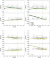 |
Fig. 11 Same as Fig. 10, but for [Pb/Eu], [Pb/O], [Eu/O], and [Eu/Fe] vs. [M/H]. |
| In the text | |
Current usage metrics show cumulative count of Article Views (full-text article views including HTML views, PDF and ePub downloads, according to the available data) and Abstracts Views on Vision4Press platform.
Data correspond to usage on the plateform after 2015. The current usage metrics is available 48-96 hours after online publication and is updated daily on week days.
Initial download of the metrics may take a while.