| Issue |
A&A
Volume 690, October 2024
|
|
|---|---|---|
| Article Number | A204 | |
| Number of page(s) | 15 | |
| Section | Astronomical instrumentation | |
| DOI | https://doi.org/10.1051/0004-6361/202450775 | |
| Published online | 10 October 2024 | |
Eighteen new fast radio bursts in the High Time Resolution Universe survey
1
INAF – Osservatorio Astronomico di Cagliari,
via della Scienza 5,
09047
Selargius (CA),
Italy
2
ARC Center of Excellence for Gravitational Wave Discovery (OzGrav), Swinburne University of Technology,
Mail H11, PO Box 218,
Hawthorn,
VIC 3122,
Australia
3
Centre for Astrophysics and Supercomputing, Swinburne University of Technology,
Hawthorn,
VIC 3122,
Australia
4
School of Physics, Trinity College Dublin, College Green,
Dublin 2,
D02 PN40,
Ireland
5
Max-Planck-Institut für Radioastronomie,
Auf dem Hügel 69,
53121
Bonn,
Germany
6
Jodrell Bank Center for Astrophysics, University of Manchester,
Alan Turing Building, Oxford Road,
Manchester
M13 9PL,
UK
7
ASTRON, Netherlands Institute for Radio Astronomy,
Oude Hoogeveensedijk 4,
7991 PD
Dwingeloo,
The Netherlands
8
Joint institute for VLBI ERIC,
Oude Hoogeveensedijk 4,
7991 PD
Dwingeloo,
The Netherlands
9
Anton Pannekoek Institute for Astronomy, University of Amsterdam,
Science Park 904,
1098 XH
Amsterdam,
The Netherlands
10
CSIRO Astronomy & Space Science, Australia Telescope National Facility,
PO Box 76,
Epping,
NSW 1710,
Australia
11
International Centre for Radio Astronomy Research, Curtin University,
Perth,
WA,
Australia
12
Australia Telescope National Facility, CSIRO Space and Astronomy,
PO Box 76,
Epping,
NSW 1710,
Australia
13
Laboratoire de Physique et Chimie de l'Environnement et de l'Espace – Université d'Orléans/CNRS,
45071,
Orléans Cedex 02,
France
14
Center for Gravitation, Cosmology, and Astrophysics, Department of Physics, University of Wisconsin-Milwaukee,
PO Box 413,
Milwaukee,
WI 53201,
USA
★ Corresponding author; This email address is being protected from spambots. You need JavaScript enabled to view it.
Received:
17
May
2024
Accepted:
23
August
2024
Abstract
Context. Current observational evidence reveals that fast radio bursts (FRBs) exhibit bandwidths ranging from a few dozen MHz to several GHz. Traditional FRB searches primarily employ matched filter methods on time series collapsed across the entire observational bandwidth. However, with modern ultrawideband receivers featuring gigahertz-scale observational bandwidths, this approach may overlook a significant number of events.
Aims. We investigate the efficacy of sub-banded searches for FRBs, whereby we look for bursts within limited portions of the bandwidth. The aim of these searches is to enhance the significance of FRB detections by mitigating the impact of noise outside the targeted frequency range, thereby improving signal-to-noise ratios.
Methods. We conducted a series of Monte Carlo simulations for the 400-MHz bandwidth Parkes 21-cm multi-beam (PMB) receiver system and the Parkes Ultra-Wideband Low (UWL) receiver, simulating bursts down to frequency widths of about 100 MHz. Additionally, we performed a complete reprocessing of the high-latitude segment of the High Time Resolution Universe South survey (HTRU-S) of the Parkes-Murriyang telescope using sub-banded search techniques.
Results. Simulations reveal that a sub-banded search can enhance the burst search efficiency by 67−42+133% for the PMB system and 1433−126+143% for the UWL receiver. Furthermore, the reprocessing of HTRU led to the confident detection of 18 new bursts, nearly tripling the count of FRBs found in this survey.
Conclusions. These results underscore the importance of employing sub-banded search methodologies to effectively address the often modest spectral occupancy of these signals.
Key words: methods: data analysis / surveys
© The Authors 2024
 Open Access article, published by EDP Sciences, under the terms of the Creative Commons Attribution License (https://creativecommons.org/licenses/by/4.0), which permits unrestricted use, distribution, and reproduction in any medium, provided the original work is properly cited.
This article is published in open access under the Subscribe to Open model. This email address is being protected from spambots. You need JavaScript enabled to view it. to support open access publication.
1 Introduction
Fast radio bursts (FRBs) are Jy-intensity radio flashes with milliseconds durations. They primarily exhibit dispersion measures (DMs) that greatly exceed the contribution from the Galaxy (Thornton et al. 2013), and are therefore (mostly) extragalactic sources (for recent reviews, see e.g. Bailes 2022; Petroff et al. 2022). After the initial discovery of the first FRB event by Lorimer et al. (2007), the first population of bursts was reported in 2013 by Thornton et al. (2013). This discovery was made by analysing a subset of data from the high-latitude portion of the High Time Resolution Universe (HTRU, Keith et al. 2010) survey conducted using the 64-m single-dish Parkes-Murriyang telescope in Australia. Subsequently, the field experienced rapid growth. Notably, the identification of repeating sources (e.g. Spitler et al. 2016; CHIME/FRB Collaboration 2019) facilitated dedicated large-scale campaigns, enabling precise localisation and host galaxy identification (Marcote et al. 2017; Tendulkar et al. 2017; Marcote et al. 2020; Kirsten et al. 2022), the discovery of periodic activity in two repeaters (Chime/FRB Collaboration 2020; Rajwade et al. 2020), and the detection of emission with nanosecond duration (Nimmo et al. 2021, 2022; Majid et al. 2021; Snelders et al. 2023).
Blind searches for these transient events are usually carried out by searching for excesses in the time series of the recorded signal via matched filtering (Cordes & McLaughlin 2003; Qiu et al. 2023). After extracting the Stokes I spectrogram from the original complex voltage of the signal, the essential steps of a FRB search pipeline are as follows: (i) The data are initially cleaned to remove radio frequency interference (RFI) signals that can disrupt the burst search if not properly eliminated. (ii) The Stokes I matrix is subsequently adjusted for several trial DMs by shifting each channel row according to the corresponding DM-induced delay. (iii) A flat spectral index is then assumed for the FRB emission and the DM-corrected matrices are averaged per frequency. (iv) The time series is then convolved with top-hat functions using various trial boxcar widths, while candidates above a given signal-to-noise ratio (S/N) threshold are retained. (v) Temporally coincident candidates are then clustered, matching DM/boxcar widths into a single event. (vi) Finally, the grouped events are vetted with either an artificial intelligence (AI) classifier (see e.g. Connor & van Leeuwen 2018; Agarwal et al. 2020) or by human inspection.
In contrast to pulsars, which display broad fractional band-widths (Jankowski et al. 2018) – in some extreme cases extending to 100 GHz (Torne et al. 2022) –, the spectral occupancy of FRBs appears in many case to be narrower. This effect seems particularly pronounced for the repeater class, and is less evident in the isolated 'one-off' bursts, suggesting the possibility of a morphological dichotomy between the two classes of FRBs (Pleunis et al. 2021).
Furthermore, the repeaters' bandwidths appear to be frequency-dependent. For instance, FRB 20121102A exhibits bandwidths of a few hundred MHz at 1.4 GHz (Hewitt et al. 2022) and broadens to the order of gigahertz for bursts at 6 GHz (Gajjar et al. 2018). A similar trend is observed for FRB 20180916B, where bursts at 0.6 GHz show bandwidths of hundreds of MHz (Sand et al. 2022), reaching bandwidths spanning GHz for bursts at 4.5 GHz (Bethapudi et al. 2023).
Observations with receivers possessing extremely large observational bandwidths could provide a definitive answer to the question of whether or not this dichotomy in bandwidths between repeaters and one-off events truly exists. If these results hold for larger samples of bursts, they could also help answer the question of whether or not repeating FRBs and one-off FRBs indeed constitute separate classes of events, as this distinction might not exist (James 2023).
Due to the narrower spectral occupancy of FRBs compared to the full observational bandwidth, searching for signal excesses in the frequency-averaged time series of the entire band might be expected to introduce excessive noise. This situation could potentially cause the burst signal to fall below the S/N threshold. This issue is particularly pronounced with modern receivers like the Parkes Ultra-Wideband Low (UWL, Hobbs et al. 2020), which boasts an observational bandwidth of approximately 3.3 GHz. A practical approach to avoid missing events that occupy a significantly smaller portion of the full observational bandwidth involves conducting a sub-banded search. This method entails searching for bursts in a manner akin to the previous discussion, but focusing on smaller portions of the data matrix in terms of frequency. This process is then iteratively applied across all sub-bands. For instance, this technique enabled Kumar et al. (2021) to identify a very narrow burst with a bandwidth of about 65 MHz from the repeater FRB 20180711A within the UWL data.
The aim of this work is to provide a comprehensive analysis of sub-banded burst searches, with a particular focus on demonstrating the potential gain in number of detections. To illustrate this concept, we conducted a Monte Carlo simulation and also performed a reprocessing of the high-latitude portion of the HTRU survey, resulting in the discovery of 18 new FRBs. The structure of this paper is as follows: Sect. 2 outlines the framework for sub-banded searches and a description of our simulations; Sect. 3 provides a concise overview of the HTRU survey and details the software pipeline we developed for processing; Sect. 4 presents the outcomes of our reprocessing; and finally, Sect. 5 provides a summary and concluding remarks.
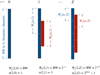 |
Fig. 1 Strategy for the FRB sub-banded search (see Sect. 2.1). The full band BW is iteratively divided up into sub-bands Wv(a, Z), given a certain partition factor and partition exponent (represented here as blue rectangles). Overlapping sub-bands (red rectangles) are considered in order to search for events that occupy adjacent sub-bands. |
2 Sub-banded search algorithm
2.1 Design
The design of a sub-banded search algorithm can be done in various ways, each tailored to specific scientific results one wants to achieve. One possible approach involves segmenting the entire observational bandwidth into distinct sub-bands of varying sizes. If the burst is fully contained in a given sub-band Wv, assuming a Gaussian-shaped spectrum with full width at half maximum (FWHM) Wv, it can be shown that (see Appendix A):
![Mathematical equation: $\[\mathrm{S} / \mathrm{N}^* \simeq \sqrt{\frac{\mathrm{BW}}{W_\nu}} \mathrm{~S} / \mathrm{N},\]$](/articles/aa/full_html/2024/10/aa50775-24/aa50775-24-eq3.png) (1)
(1)
where S/N* and S/N are the signal-to-noise ratios in the given sub-band and in the full band BW respectively. In this context, we present a procedural framework for sub-banded searches, visually outlined in Fig. 1. We consider a channelised spectrogram with Nc frequency channels, within an observational band BW. We evenly divide the total observational bandwidth into az sub-bands, where z = 0, 1,..., Z, with a the partition factor and Z the partition exponent. Consequently, for each z, each sub-band possesses a bandwidth:
![Mathematical equation: $\[W_\nu(a, z)=\mathrm{BW} \times a^{-z}.\]$](/articles/aa/full_html/2024/10/aa50775-24/aa50775-24-eq4.png) (2)
(2)
As depicted in Fig. 1, we also consider, for each z, equally large Wv(a, z) adjacent sub-bands. This is done in order to mitigate the possibility of missing events that might manifest between adjoining sub-bands. The number of sub-bands n(a, z) produced in a given exponent z is simply:
![Mathematical equation: $\[n(a, z)=2 a^z-1.\]$](/articles/aa/full_html/2024/10/aa50775-24/aa50775-24-eq5.png) (3)
(3)
The overall count of sub-bands N(a, Z) to be processed can be calculated as:
![Mathematical equation: $\[N(a, Z)=\sum_{z=0}^Z n(a, z)=\frac{2 a^{Z+1}-a(Z+1)+Z-1}{a-1}.\]$](/articles/aa/full_html/2024/10/aa50775-24/aa50775-24-eq6.png) (4)
(4)
For example, let us consider a = 2 and Z = 2. This configuration encompasses the entire observational band BW, three bands each constituting half of BW, and seven bands each occupying one-quarter of BW. Consequently, a total of 11 bands require processing.
The choice of the parameters a and Z necessitates a compromise between the desired sub-band width Wv(a, Z) one wants to search for bursts and the manageable count of total searches N(a, Z), as this exponentially increases for large values of Z.
2.2 Detection gain
To assess the increased detection capability of the sub-banded search discussed in Sect. 2.1, we conducted two Monte Carlo experiments. These simulations focused on two receivers: the Parkes 21-cm multi-beam receiver system (PMB, Staveley-Smith et al. 1996), which records data at the central frequency of 1382 MHz with an observational bandwidth of 400 MHz, and the UWL, which is centred at 2368 MHz within a 3328 MHz band. In order to have comparable results with the real data application discussed in Sect. 3.2, we consider an effective bandwidth for the PMB of 340 MHz.
In both simulations, an FRB event was generated as a Gaussian function G(v; {v0, Δv, Fv}). This function is characterised by three parameters: v0, the central emission frequency corresponding to the Gaussian centroid; Δv, the Gaussian FWHM representing the burst frequency width; and Fv, the burst fluence, calculated as ∫ G(v)dv.
In the sub-banded search, the fluence is evaluated within limited frequencies v1, v2, as described in Sect. 2.1. If the fluence ![Mathematical equation: $\[\int_{\nu_1}^{\nu_2} G(\nu) d \nu\]$](/articles/aa/full_html/2024/10/aa50775-24/aa50775-24-eq7.png) in one of the sub-bands exceeds the telescope radiometer fluence sensitivity (with a S/N threshold of 10), improved by a factor of BW/(v2 − v1) (see Eqs. (A.18), (A.19)), the event is labelled as detected.
in one of the sub-bands exceeds the telescope radiometer fluence sensitivity (with a S/N threshold of 10), improved by a factor of BW/(v2 − v1) (see Eqs. (A.18), (A.19)), the event is labelled as detected.
For both experiments, some parameters are drawn randomly, while others are kept fixed. Below, we describe the simulation parameters.
Experiment 1: We produced 104 bursts, whose parameters {v0, Δv, Fv} are randomly generated. Fluences are drawn from a power-law distribution between the receiver's sensitivity fluence of 0.6 Jy ms and 103 Jy ms, assuming a slope of −3/2. Considering current evidence for FRB bandwidths, we generated widths uniformly 𝒰 distributed in the range 70–1000 MHz for both receivers. Frequency centroids are drawn from uniform distributions 𝒰(400, 1900) MHz and 𝒰(400, 4400) MHz for the PMB and UWL, respectively. The ranges are slightly larger than the receiver's band in order to consider outside-band events whose spectral widths are large enough to significantly occupy the receiver's band. For each event, we performed a full-band search and a sub-banded search with parameters a = 2, Z = 2 for the PMB and a = 2, Z = 6 for the UWL. After counting the number of detected bursts for both searches and receivers, we repeated the experiment for 103 trials. The aim of this experiment is to provide a prediction of the gain in detections when performing a sub-banded search compared to a full-band search, given a certain sub-banded search setup and for a given dataset, and assuming no prior knowledge of the bandwidth occupancy of the putative bursts in the data.
Experiment 2: In this case, we keep fixed the percentage bandwidth occupancy of the bursts (hereafter referred to as the spectral widths), considering the following bandwidth occupancies: [10, 20, 25, 40, 50, 60, 75, 80, 90, 95, 99, 99.9, 99.99]% for the PMB and [1, 2, 2.5, 4, 5, 6, 7.5, 8, 10, 20, 25, 40, 50, 60, 75, 80, 90, 95, 99, 99.9, 99.99]% for the UWL. For each fixed occupancy, we generated 104 bursts, with fluences distributed as previously described and with frequency centroid uniformly distributed within the receiver bandwidth, ensuring that each burst is fully contained within the band. We again performed a full-band search and a sub-banded search with the same parameter setup, counted the detected events, and performed 103 repeat trials for each spectral occupancy. With this experiment, the aim is to evaluate the detection gain as a function of the burst percentage occupancy.
Figure 2 illustrates the results of the two Monte Carlo experiments. The top panel displays the detection gain distributions from Experiment 1 for both PMB and UWL. The UWL gain distribution is approximately Gaussian, centred around ~1400%, while the PMB gain distribution is positively skewed, with a median gain of 67%. This skewness in the PMB gain distribution is expected, given our priors for the width distribution. A substantial portion of the generated events occupy the entire observational bandwidth of the PMB, shifting the gain toward lower values. In contrast, for the UWL, this scenario never occurs for construction, as the widest bursts would only occupy about 30% of the UWL bandwidth.
From these results, we can establish an overall detection gain for both receivers, considering the sub-banded search setup used. Assuming the 16–84 percentile range of our distribution as a 1σ uncertainty, we obtain an overall detection gain of ![Mathematical equation: $\[\mathcal{G}_{\mathrm{PMB}}=67_{-42}^{+133} \%\]$](/articles/aa/full_html/2024/10/aa50775-24/aa50775-24-eq8.png) for the PMB and
for the PMB and ![Mathematical equation: $\[\mathcal{G}_{\mathrm{UWL}}=1433_{-126}^{+143} \%\]$](/articles/aa/full_html/2024/10/aa50775-24/aa50775-24-eq9.png) .
.
The bottom panel of Fig. 2 depicts the detection gain as a function of burst occupancy. For very low occupancies, such as the case of 2% for the UWL (as in the burst detected by Kumar et al. 2021), the detection gain becomes remarkably high, reaching ~6000%. This implies that, given a certain UWL dataset, if a full-band search detects a single event, a sub-banded search with a = 2 and Z = 6 could potentially allow the detection of 60 more events. Conversely, as we approach occupancies of greater than 90%, the detection gain for both receivers dramatically decreases to zero.
3 Reprocessing of the HTRU South survey
3.1 Observations
As a real-data application, we reprocessed the HTRU survey using the sub-banded search algorithm. The HTRU survey is an all-sky survey designed for discovering pulsars and fast transients. It consists of two parts: one carried out with the Parkes–Murriyang telescope, which covered the Southern hemisphere of the Sky (HTRU-S), and the other made by the 100-m single dish Effelsberg telescope in Germany to cover the Northern Sky (HTRU-N). In the present work, we focus on HTRU South and refer readers to Barr et al. (2013) for a complete overview of the observational setup and strategy for HTRU North.
The HTRU South survey is divided into three surveys, each covering a different region of the Sky: the low-latitude (LowLAT) survey, which covers the sky area of Galactic longitude −80° < l < +30° at Galactic latitudes −3.5° < b < +3.5°; the mid-latitude (MedLAT) survey, which comprises the region of −120° < l < +30° and −15° < b < +15°; and lastly the high-latitude (HiLAT) survey, which covers the entire region of the Southern Sky with declination δ < 10°. In this work, we focus on HiLAT, which is specifically designed for extragalactic radio transients.
The data were recorded with the PMB receiver. The PMB consists of 13 feeds centred around the prime focus of the Parkes antenna organised as two concentric sets of hexagons. The HTRU HiLat data are recorded as 2 bits total-intensity search-mode SIGPROC filterbanks (Lorimer 2011). Each filterbank file possesses 1024 frequency channels of bandwidth dv = 390.626 kHz and sampled at dt = 64 μs each. Each observation lasted 270 s.
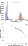 |
Fig. 2 Results of the Monte Carlo experiments (see Sect. 2.2 for more details). The top panel a displays the distribution of the detection gain obtained by performing a sub-banded search over a full-band search (Experiment 1), both for the PMB (violet, search parameters a = 2 and Z = 2) and UWL (coral, search parameters a = 2, Z = 6) receivers. The dashed vertical lines represent the distribution percentiles at 16, 50, and 84%. The bottom panel b illustrates the sub-banded search detection gain as a function of the burst bandwidth occupancy (Experiment 2). The colour code and the sub-banded search parameters are the same as the top panel. |
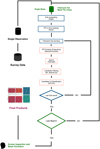 |
Fig. 3 Flow chart of the sub-band search pipeline deployed to process the HTRU HiLAT. |
3.2 Data analysis
To process the HiLAT segment of the survey, we developed a dedicated pipeline, which is outlined in Fig. 3. Data processing was executed using the OzSTAR supercomputer1 hosted at Swinburne University in Australia. Each observation comprised 13 individual SIGPROC filterbank files, one for each beam of the PMB receiver. The processing sequence for each filterbank file involved the following steps:
File upsampling. As a first step, the filterbank file is upsampled from a 2 bits file to an 8 bits file using the software routine digifil from the DSPSR software package (van Straten & Bailes 2011). This step is necessary in order to make the data readable by the AI classifier at later stages.
RFI excision in time. Accompanying each filterbank file is an RFI mask detailing the worst-affected time bins (see Keith et al. 2010, Sect. 4.1.1). Corrupted bins are replaced with random Gaussian numbers drawn from the distribution of uncorrupted time bins. This process is executed via the filedit routine from SIGPROC.
File sub-banding and processing. Each file is sub-banded according to the procedure outlined in Sect. 2.1 and we considered a partition factor of α = 2 and a partition exponent of Z = 2, which yielded the following configuration of sub-bands: 1 × 400 MHz, 3 × 200 MHz and 7 × 100 MHz. This was done in order to obtain a compromise between search sensitivity and computation time. For each sub-band, we then processed the data according to the following steps:
- (i)
For each sub-banded file, we search for the noisiest channels present in the data. We adopted a Spectral Kurtosis algorithm (provided by the python package your, Aggarwal et al. 2020). As previously mentioned in Sect. 2.2, about 60 MHz (~154 channels) of the top band is known to be always affected by RFI due to the presence of satellite telemetry. These channels were always flagged as zero.
- (ii)
We searched for FRB candidates via the software package HEIMDALL (Barsdell et al. 2012). As HEIMDALL performs its own RFI flagging, we parsed the previously computed corrupted channels via the option -zap_chans to ensure a further RFI excision. The data were searched in DM from 0 to 5000 pc cm−3, over box-car widths from 0.128 ms (2 bins) to 262.144 ms (4096 bins).
- (iii)
Before using an AI classification, we made a pre-filtering step to significantly reduce the sheer amount of candidates produced by HEIMDALL by matching the following criteria:
![Mathematical equation: $\[\begin{aligned}\mathrm{S} / \mathrm{N} & \geq 7; \\\mathrm{DM} & \geq 10 \mathrm{pc} \mathrm{~cm}^{-3}; \\N_m & \geq 3; \\N_{\mathrm{ls}} & \leq 2,\end{aligned}\]$](/articles/aa/full_html/2024/10/aa50775-24/aa50775-24-eq10.png) (5)
(5)where Nm is the minimum number of distinct boxcars/DM trials clustered into a single candidate by HEIMDALL and N1s is the maximum number of candidates permitted in a window of 1s in length. The last two criteria were used to mitigate events most likely caused by noise fluctuations and RFI storms, respectively. However, the latter could have filtered out second-long events like those reported by CHIME (Chime/FRB Collaboration 2022), a trade-off we accepted between missing some events and reducing the number of probable false positives passed to the classifier. This selection process was implemented using the software frb_detector.py (Barsdell et al. 2012).
- (iv)
Subsequently, candidates satisfying the criteria detailed in Eq. (5) were subjected to scrutiny by FETCH (Agarwal et al. 2020). FETCH is an AI classifier that offers 11 convolutional neural network architectures (referred to as models a to k), each with a distinct configuration of layers (for details, see Agarwal et al. 2020). Model a was exclusively employed, as it was reported by the authors as the most effective overall.
- (i)
Human evaluation. Lastly the candidates positively classified by FETCH are evaluated by visual inspection. The following criteria we used. As a conservative approach, all the candidates that showed bright clustered pixels in the dynamic spectrum (in addition to the clustered ones of the putative FRB candidate) were discarded. This is done conservatively to avoid possible RFI signals that are temporally too close to the single pulse candidates. Candidates with a DM compatible with the Galactic DM predicted using the NE2001 (Cordes & Lazio 2002) model and YMW16 (Yao et al. 2017) for the beam sky direction were also rejected; we plan to vet them (e.g. positively classify them as new pulsars or rotating radio transients, RRATs) as part of a future work, which will comprise the reprocessing of LoLAT and MedLAT. Candidates that appeared in multiple but non-adjacent beams according to the geometry of the PMB were not considered.
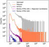 |
Fig. 4 S/N distributions (binned with an S/N bin size of 1) of the candidates: in grey, those initially detected by HEIMDALL; in coral, the HEIMDALL candidates filtered according to the criteria listed in Eq. (5); in purple, the filtered candidates positively classified by FETCH; in magenta, the sample of our 51 detections along with the 10 previously discovered FRBs in this survey (Thornton et al. 2013; Champion et al. 2016; Petroff et al. 2019, including detections in multiple sub-bands); and in blue, the same distribution as the magenta one, but with the sample of our detections limited to events with S/N ≥ 10 (see Sect. 4.2 for more details). |
4 Results and discussion
4.1 Redetected bursts
Following the complete processing, HEIMDALL identified approximately 6 × 10⁹ candidates (above a S/N ≥ 6), of which approximately 107 survived the pipeline filtering steps as discussed in Sect. 3.2. Only ~104 of these were positively classified by FETCH (See Fig. 4).
We redetected the ten previously discovered FRBs in the HiLAT region (Thornton et al. 2013; Champion et al. 2016; Petroff et al. 2019), both in the full-band and across several subbands. Notably, the S/N values of these sub-banded bursts, such as those from FRB 20110220A, provide significant insights. The burst in the full-band exhibits an S/N of approximately 49. Interestingly, this burst has an S/N of ~70% of the full-band S/N if we consider half sub-bands (see Fig. 5) and about 50% of the full-band S/N in the quarter sub-bands. We therefore observe a S/N loss rather than a gain. A similar scenario applies for FRB 20130626A. In contrast, we observe that FRB 20110127A, 20130729A, and 20110214A exhibit a higher S/N in the lower half band, as the majority of their signal is concentrated in this frequency range (this was already noted for FRB 20110214A; see Petroff et al. 2019). With the exception of these three bursts, the spectra of all published FRBs span the entire observational bandwidth. In such instances, it can be shown (see Appendix A) that if the burst fully occupies the observational bandwidth, Eq. (1) assumes the form
![Mathematical equation: $\[\mathrm{S} / \mathrm{N}^* \simeq \sqrt{\frac{W_\nu}{\mathrm{BW}}} \mathrm{~S} / \mathrm{N}.\]$](/articles/aa/full_html/2024/10/aa50775-24/aa50775-24-eq11.png) (6)
(6)
This conclusion is consistent with the aforementioned bursts from Thornton et al. (2013) and Champion et al. (2016), and it reasonably applies to all seven full-band HiLAT bursts, albeit with certain discrepancies that could arise mainly due to the presence of RFI or the limitations of the burst model. Another factor could be the assumption that, as initially discussed in Sec. 1, we assume a flat spectral index for the FRB emission, that is, when collapsing the Stokes I matrix to get the time series to be searched for, we do not weight each channel of central frequency v for a factor of the kind (v/v0)β, where v0 is a reference frequency and β the spectral index. To test this, we considered FRB 20110220A, which is the strongest burst of the HTRU sample, and recomputed the S/N of the burst by considering trial spectral index values in the range of (−10, 10). We notice that the S/N peaks at β ≃ 2, but it results in an S/N improvement of less than 1%.
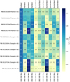 |
Fig. 5 Recomputed relative S/N (normalised for the full-band S/N) for each sub-band processed in the search and for each of the previously detected HTRU FRBs. For each burst, the relative sub-band has been considered, and the S/N computed using Eq., (A.4). |
4.2 New detections
Among the 104 candidates that successfully passed the FETCH selection, and excluding the previous 10 discovered FRBs, only 51 fulfilled the criteria outlined in the human vetting section of the pipeline. Our identified candidates exhibit sub-band S/N values ranging from 7 (the minimum allowable value according to our filtering criteria) to 12.
We first discuss the probability that these bursts are simply due to random excesses in the frequency-averaged time series. Cordes & McLaughlin (2003) showed that, for a time series of Ns samples, the average number of false detections nfalse(> S/N) -by chance due only to noise – for a single DM trial and above a certain S/N is
![Mathematical equation: $\[n_{\text {false }}(>\mathrm{S} / \mathrm{N}) \simeq 2 N_s P(>\mathrm{S} / \mathrm{N}) \text {, }\]$](/articles/aa/full_html/2024/10/aa50775-24/aa50775-24-eq12.png) (7)
(7)
where
![Mathematical equation: $\[P(>\mathrm{S} / \mathrm{N})=\int_{\mathrm{S} / \mathrm{N}}^{+\infty} \frac{1}{\sqrt{2 \pi}} e^{-\frac{x^2}{2}} d x=\frac{1}{2}\left[1-\operatorname{erf}\left(\frac{\mathrm{S} / \mathrm{N}}{\sqrt{2}}\right)\right],\]$](/articles/aa/full_html/2024/10/aa50775-24/aa50775-24-eq13.png) (8)
(8)
and erf(x) is the error function. When processing a survey of Npoint pointings of Nbeam beams each and searching for bursts via a sub-banded search processing a total number of sub-bands Nsub, the total number of false detections Nfalse(> S/N) above a certain S/N is
![Mathematical equation: $\[N_{\text {false }}(>\mathrm{S} / \mathrm{N}) \simeq 2 N_{\text {beam }} N_{\text {point }} N_s P(>\mathrm{S} / \mathrm{N}) \Pi\left(N_{\mathrm{DM}}\right),\]$](/articles/aa/full_html/2024/10/aa50775-24/aa50775-24-eq14.png) (9)
(9)
where
![Mathematical equation: $\[\Pi\left(N_{\mathrm{DM}}\right)=\sum_{\text {all sub-bands }} n_{\mathrm{DM}}\left(\nu_{\text {top }}, \nu_{\text {bot }}\right)\]$](/articles/aa/full_html/2024/10/aa50775-24/aa50775-24-eq15.png) (10)
(10)
is the total number of DM trials searched for each sub-band2 with top and bottom frequency vtop and vbot, respectively.
Employing Eq. (9) and considering our survey specifics and the sub-banded search strategy, we expect less than one candidate to be detected by random chance due to noise for sub-banded S/N > 8.2 (see Appendix B). However, it is advisable to set a slightly higher S/N threshold than the computed value in order to account for the inherent uncertainty in the S/N estimation, which has an error of 1 (see again Appendix B for further details). This adjustment helps ensure that candidates close to the noise floor are not mistakenly considered as detections.
Additionally, the presence of RFI could significantly impact the effectiveness of the S/N threshold, as the unpredictable nature of RFI can lead to an increased number of false detections. Accurately quantifying how RFI might affect our results requires a comprehensive understanding of the specific RFI environment, which is beyond the scope of this work.
Another important factor to consider is the performance of the classifier. As indicated by the authors, FETCH achieves a recall rate3 exceeding 99% for S/N values of greater than 10. Therefore, aligning the S/N threshold with this optimal range not only mitigates the effects of noise and RFI but also ensures that the classifier performs effectively.
Given this, we conservatively positively vetted candidates with S/N ≥ 10 (18 out of 51 of our candidates) as probable detections. The remaining candidates were rejected. Table C.1 shows the properties of the detected bursts (in addition to the already discovered ones), named BXX, and Fig. 6 depicts the waterfall plots of the five highest sub-band S/N bursts (see Appendix C for the remaining ones). The DM of these candidates spans a range from a minimum of approximately 200 pc cm−3 to a maximum of about 1650 pc cm−3, which is 2 to 30 times larger than the DM predictions for the Galactic contribution in their respective beam pointings (obtained using the software package PYGEDM, Price et al. 2021). With these additional 18 detections, along with the 10 previous discoveries, the sub-banded search exhibited a detection gain of 180%. Despite being notably high for the 400 MHz band of the PMB, this value still aligns well with the predicted detection gain discussed in Sect. 2.2 for the PMB, falling within the 1σ range error, further enhancing the significance of the candidates.
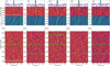 |
Fig. 6 Narrow-band bursts detected in the HTRU HiLAT sub-band search. Here, we display the five highest sub-band S/N (see Appendix C for the remaining candidates). For each burst, the bottom panel shows the dedispersed waterfall plot of the data, with two green lines delimiting the sub-band area in which the burst has been detected. The central lower panel shows the DM-time (butterfly) plot of the burst, and the central upper panel is the waterfall plot of the sub-banded dedispersed data. Lastly, the top panel shows the frequency-averaged time series along the sub-band. The blank rows in all the waterfall plots represent excised channels due to RFI. |
4.3 Parameter distributions
Figure 7 shows the parameter distribution of the HTRU bursts, which comprise the 18 new detections and the published bursts. As a comparison, for the DM and burst time width distribution, we also show the sample of one-off FRBs published in the first CHIME/FRB catalogue (CHIME/FRB Collaboration 2021), the sample of one-off bursts published by ASKAP (Shannon et al. 2018; Bannister et al. 2019; Macquart et al. 2019; Prochaska et al. 2019; Bhandari et al. 2023; Ryder et al. 2023), and the sample of FRBs discovered by UTMOST (Caleb et al. 2017; Farah et al. 2019; Gupta et al. 2019a,b,c, 2020a,b; Mandlik et al. 2021, 2022). The data were retrieved from the on-line database FRB STATS (Spanakis-Misirlis 2021). Each pair of histograms is accompanied by the Kolmogorov-Smirnov probability pKS that the two are drawn from the same distribution.
Regarding the DM distribution, from Fig. 7, we see that the Parkes HTRU distribution tends to peak at ~500 pc cm−3, with the shape being consistent with a log-normal distribution, as similarly obtained by CHIME/FRB, ASKAP, and UTMOST. This also applies for the time width distribution, with a peak around widths of 2–4 ms. In the case of the frequency width distributions, we do not make a comparison with either of the other samples, because we followed a different search strategy in order to carry out the sub-banded search. The last two histograms of Fig. 7, as well as Fig. 8, show the sky distribution of the beam pointings of the detected bursts. The distributions are relatively uniform. We notice that there are fewer detections in the range −15° < b < 15°, which is consistent with the design of HiLAT, as discussed in Sect. 3.1.
In Fig. 7 (panel f), we display the distribution of the times of arrival of our 18 detections, as local time in Australian Eastern Standard Time (AEST). This figure was built in order to check whether or not our new sample could be ascribed to the class of peryton signals (Burke-Spolaor et al. 2011; Kocz et al. 2012; Bagchi et al. 2012), an FRB-like signal that turned out to be RFI (Petroff et al. 2015) from a microwave oven. Perytons are characterised as strong bursts (usually detected in multiple non-adjacent beams of the PMB) frequency-sweeped closely to a v−2 relation, giving them an 'apparent' DM usually clustered around ~400 pc cm−3 or slightly less commonly around ~200 pc cm−3. The ultimate test to establish their terrestrial nature was in fact to display their occurrence within the time of day, noticing that they tend to cluster during the typical lunch and dinner hours at the Parkes facility (see, Petroff et al. 2015). From Fig. 7 (panel f), we see that the distribution is relatively uniform, which, in addition to our multi-beam exclusion criteria discussed in Sect. 3.2, supports the idea that it is unlikely that our candidates are weak perytons.
Lastly, using the sample of 28 FRBs, following Thornton et al. (2013) and Champion et al. (2016) we estimate an updated all-sky rate for HiLAT of
![Mathematical equation: $\[R\left(>F_\nu \sim 0.6 ~\mathrm{Jy} \mathrm{~ms}\right)=4 \pi\left(\frac{N_{\mathrm{FRBs}}}{0.0197}\right) \mathrm{sky}^{-1} \text { day }^{-1},\]$](/articles/aa/full_html/2024/10/aa50775-24/aa50775-24-eq16.png) (11)
(11)
which returns a rate of ![Mathematical equation: $\[1.8_{-0.3}^{+0.4} \times 10^4\]$](/articles/aa/full_html/2024/10/aa50775-24/aa50775-24-eq17.png) sky−1 day−1 for NFRBs = 28 (with uncertainties at 1σ c.l. assuming Poissonian statistics; Gehrels 1986). The obtained value, scaled with respect to the Parkes completeness fluence of ~2 Jy ms (Keane & Petroff 2015) and assuming a Euclidean fluence slope of −3/2, is consistent with the Parkes all-sky rate reported by Bhandari et al. (2018), of namely
sky−1 day−1 for NFRBs = 28 (with uncertainties at 1σ c.l. assuming Poissonian statistics; Gehrels 1986). The obtained value, scaled with respect to the Parkes completeness fluence of ~2 Jy ms (Keane & Petroff 2015) and assuming a Euclidean fluence slope of −3/2, is consistent with the Parkes all-sky rate reported by Bhandari et al. (2018), of namely ![Mathematical equation: $\[1.7_{-1.1}^{+1.5} \times 10^3\]$](/articles/aa/full_html/2024/10/aa50775-24/aa50775-24-eq18.png) sky−1 day−1.
sky−1 day−1.
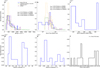 |
Fig. 7 Distributions of DM (a), burst time width (b), burst frequency width (c), Galactic Latitude b (d), and Galactic Longitude l (e). The Parkes sample (blue) consists of our 18 detections along with the 10 already discovered FRBs in this survey (Thornton et al. 2013; Champion et al. 2016; Petroff et al. 2019). For subplots (a, b), we also display, for comparison, the distribution obtained by considering the sample of the one-off FRBs published by CHIME (green, CHIME/FRB Collaboration 2021), the distribution of the sample of ASKAP one-off FRBs (orange, Shannon et al. 2018; Bannister et al. 2019; Macquart et al. 2019; Prochaska et al. 2019; Bhandari et al. 2023; Ryder et al. 2023), and the sample of FRBs detected by UTMOST (violet, Caleb et al. 2017; Farah et al. 2019; Gupta et al. 2019a,b,c, 2020a,b; Mandlik et al. 2021, 2022). For each pair of histograms in each subplot, we report the Kolmogorov-Smirnov probability pKS of being drawn from the same distribution. Panel (f) shows the distribution of the newly detected burst arrival times in AEST local time. |
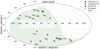 |
Fig. 8 Sky distribution (Aitoff projection) of the bursts detected in this work via the sub-banded search of HTRU HiLAT. For comparison, the bursts from Thornton et al. (2013); Champion et al. (2016); Petroff et al. (2019) are also plotted. |
5 Summary and conclusions
This work provides a comprehensive analysis of sub-banded searches for fast radio bursts (FRBs), which involve the detection of bursts within a specific portion of the full observational bandwidth spectrogram. Monte Carlo simulations show that a sub-banded search, designed to detect bursts down to spectral extensions of 100 MHz, can yield a detection gain of ![Mathematical equation: $\[67_{-42}^{+133} \%\]$](/articles/aa/full_html/2024/10/aa50775-24/aa50775-24-eq19.png) for the 400 MHz band Parkes 21-cm multi-beam (PMB) receiver system and of
for the 400 MHz band Parkes 21-cm multi-beam (PMB) receiver system and of ![Mathematical equation: $\[1443_{-126}^{+143} \%\]$](/articles/aa/full_html/2024/10/aa50775-24/aa50775-24-eq20.png) for the 3328 MHz band Parkes ultra-wideband low (UWL) receiver.
for the 3328 MHz band Parkes ultra-wideband low (UWL) receiver.
As a proof of concept, we applied a sub-banded search to the high-latitude portion of the HTRU South survey whose data were recorded with the PMB. Our results include the identification of 18 new FRBs. This sample is almost twice the previously reported set of discoveries (Thornton et al. 2013; Champion et al. 2016; Petroff et al. 2019), underscoring the value of sub-banded searches even for receivers with fairly limited bandwidths, such as that of the PMB.
As radio telescope technology continues to progress, many of the latest receiver systems are able to process considerably wider observational bandwidths. Notable examples in addition to the Parkes UWL are the ultrawideband receiver of the Robert C. Byrd Green Bank Telescope (GBT, Bulatek & White 2020) and the Ultra Broadband (UBB) receiver being commissioned at Effelsberg. This ongoing trend highlights the need to conduct burst searches within specific frequency ranges.
As these receiver systems incorporate larger bandwidths, alternative search strategies could come into play, such as the direct convolution of the spectro-temporal data matrix with a two-dimensional top-hat function template rather than collapsing the bandwidth (or a portion of it in a sub-banded search) and searching for excesses in the time domain. However, it is worth noting that such an approach could present computational challenges, particularly with regard to achieving real-time detections, which could be required in modern facilities, due to the impracticality of storing all the data products they generate. Considering a data matrix with Nc frequency channels and Ns time bins, a two-dimensional matched filter approach could have a time complexity of ![Mathematical equation: $\[\mathcal{O}\left(N_{\text {box }}^t N_{\text {box }}^\nu N_c N_s\right)\]$](/articles/aa/full_html/2024/10/aa50775-24/aa50775-24-eq21.png) when performing
when performing ![Mathematical equation: $\[N_{\text {box }}^t, N_{\text {box }}^\nu\]$](/articles/aa/full_html/2024/10/aa50775-24/aa50775-24-eq22.png) box-car trials in time and frequency, respectively. In contrast, a sub-banded search would require
box-car trials in time and frequency, respectively. In contrast, a sub-banded search would require ![Mathematical equation: $\[\mathcal{O}\left(N_{\text {sub }} N_{\text {box }}^t N_s\right)\]$](/articles/aa/full_html/2024/10/aa50775-24/aa50775-24-eq23.png) operations, where Nsub is the total number of sub-bands processed. In most scenarios, the sub-banded search approach would demand fewer computations and could be executed efficiently in parallel, further increasing the computational speed.
operations, where Nsub is the total number of sub-bands processed. In most scenarios, the sub-banded search approach would demand fewer computations and could be executed efficiently in parallel, further increasing the computational speed.
Acknowledgements
The authors thank the anonymous referee for the useful comments which significantly improved the quality of this work. Part of the research activities described in this paper were carried out with the contribution of the NextGenerationEU funds within the National Recovery and Resilience Plan (PNRR), Mission 4 – Education and Research, Component 2 – From Research to Business (M4C2), Investment Line 3.1 – Strengthening and creation of Research Infrastructures, Project IR0000026 – Next Generation Croce del Nord. The Parkes (Murriyang) radio telescope is part of the Australia Telescope, which is funded by the Commonwealth Government for operation as a National Facility managed by CSIRO. The reprocessing of the HTRU-S HiLat survey made an extensive use of the GPU accelerators on OzStar supercomputer at Swinburne University of Technology. The OzSTAR program receives funding in part from the Astronomy National Collaborative Research Infrastructure Strategy (NCRIS) allocation provided by the Australian Government. M. T. expresses his immense gratitude to R. Humble for assistance with the OzSTAR cluster.
Appendix A Signal-to-noise ratio enhancement
Let us consider a time series fn (with n = 0, 1,..., N − 1) of duration T. The series is then Fourier-transformed4 and modulus squared into a Nc frequency channels and Ns time bins spectrogram matrix ![Mathematical equation: $\[F^\alpha{ }_l\]$](/articles/aa/full_html/2024/10/aa50775-24/aa50775-24-eq24.png) (with α = 0, 1,..., Nc − 1; l = 0, 1,..., Ns − 1); within the frequency range vc ± BW/2, where vc is the observational central frequency and BW the observational bandwidth. We assume the spectrogram contains a candidate FRB and proceed to incoherently dedisperse the spectrogram at the correct DM value of the FRB candidate. The matrix
(with α = 0, 1,..., Nc − 1; l = 0, 1,..., Ns − 1); within the frequency range vc ± BW/2, where vc is the observational central frequency and BW the observational bandwidth. We assume the spectrogram contains a candidate FRB and proceed to incoherently dedisperse the spectrogram at the correct DM value of the FRB candidate. The matrix ![Mathematical equation: $\[F^\alpha{ }_l\]$](/articles/aa/full_html/2024/10/aa50775-24/aa50775-24-eq25.png) can be decomposed into the sum of two matrices:
can be decomposed into the sum of two matrices:
![Mathematical equation: $\[F^\alpha{ }_l=B^\alpha{ }_l+N^\alpha{ }_l,\]$](/articles/aa/full_html/2024/10/aa50775-24/aa50775-24-eq26.png) (A.1)
(A.1)
where ![Mathematical equation: $\[B^\alpha{ }_l\]$](/articles/aa/full_html/2024/10/aa50775-24/aa50775-24-eq27.png) contains only the FRB candidate signal and
contains only the FRB candidate signal and ![Mathematical equation: $\[N^\alpha{ }_l\]$](/articles/aa/full_html/2024/10/aa50775-24/aa50775-24-eq28.png) is the noise matrix. Furthermore, we assume that the initial noise in the time series fn follows a Gaussian distribution with a zero mean and variance σ2, i.e., ∈ 𝒩(0, σ2). In the matrix
is the noise matrix. Furthermore, we assume that the initial noise in the time series fn follows a Gaussian distribution with a zero mean and variance σ2, i.e., ∈ 𝒩(0, σ2). In the matrix ![Mathematical equation: $\[N^\alpha{ }_l\]$](/articles/aa/full_html/2024/10/aa50775-24/aa50775-24-eq29.png) , there will be Ns Fourier power spectral densities of Nc points, each following a gamma distribution Γ (κ, θ), with κ = 1 and θ = Ncσ2, which is therefore an exponential distribution, or equivalently, a chi-squared distribution with two degrees of freedom. This distribution possesses a mean and variance of Ncσ2 (see, e.g., Blackman & Tukey 1958, § 9, for a proof). Further processing could alter the nature of the noise. For instance, decimating the spectrogram matrix, due to the central limit theorem, will render the noise Gaussian-distributed.
, there will be Ns Fourier power spectral densities of Nc points, each following a gamma distribution Γ (κ, θ), with κ = 1 and θ = Ncσ2, which is therefore an exponential distribution, or equivalently, a chi-squared distribution with two degrees of freedom. This distribution possesses a mean and variance of Ncσ2 (see, e.g., Blackman & Tukey 1958, § 9, for a proof). Further processing could alter the nature of the noise. For instance, decimating the spectrogram matrix, due to the central limit theorem, will render the noise Gaussian-distributed.
To describe the FRB signal in the spectro-temporal domain, contained in the matrix ![Mathematical equation: $\[B^\alpha{ }_l\]$](/articles/aa/full_html/2024/10/aa50775-24/aa50775-24-eq30.png) , it is more convenient to approximate
, it is more convenient to approximate ![Mathematical equation: $\[B^\alpha{ }_l\]$](/articles/aa/full_html/2024/10/aa50775-24/aa50775-24-eq31.png) as a continuous real function B(v, t), considering that Nc >> 1 and Ns >> 1. A reasonable first approximation model for a dedispersed FRB is a two-dimensional Gaussian function of the kind:
as a continuous real function B(v, t), considering that Nc >> 1 and Ns >> 1. A reasonable first approximation model for a dedispersed FRB is a two-dimensional Gaussian function of the kind:
![Mathematical equation: $\[B^\alpha{}_l \simeq B(\nu, t)=A e^{-\frac{\left(\nu-\nu_0\right)^2}{2 \sigma_\nu^2}} e^{-\frac{\left(t-t_0\right)^2}{2 \sigma_t^2}},\]$](/articles/aa/full_html/2024/10/aa50775-24/aa50775-24-eq32.png) (A.2)
(A.2)
where A represents the amplitude controlling the signal intensity, v0, σv are the central frequency of emission and standard deviation in frequency of the burst and t0, σt are the time of arrival and standard deviation in the time of occurrence of the burst.
An important parameter for determining the significance of a burst is the S/N of the frequency-averaged profile, given by
![Mathematical equation: $\[p_l=\frac{1}{N_c} \sum_{\alpha=0}^{N_c-1} F^\alpha{ }_l.\]$](/articles/aa/full_html/2024/10/aa50775-24/aa50775-24-eq33.png) (A.3)
(A.3)
For calculating the S/N of the profile pl, we adopt the definition from Lorimer & Kramer (2005):
![Mathematical equation: $\[\mathrm{S} / \mathrm{N}=\frac{I}{\varepsilon_{\mathrm{off}} \sqrt{W_{\mathrm{eq}}}},\]$](/articles/aa/full_html/2024/10/aa50775-24/aa50775-24-eq34.png) (A.4)
(A.4)
where
![Mathematical equation: $\[I=\sum_{l=0}^{N_s}\left(p_l-\mu_{\mathrm{off}}\right).\]$](/articles/aa/full_html/2024/10/aa50775-24/aa50775-24-eq35.png) (A.5)
(A.5)
Here, μoff and ϵoff represent the mean and standard deviation of the off-pulse profile pl, and Weq is given by
![Mathematical equation: $\[W_{\mathrm{eq}}=\frac{1}{p_{z_{t_0}}} \sum_{\text {on pulse }}\left(p_l-\mu_{\mathrm{off}}\right),\]$](/articles/aa/full_html/2024/10/aa50775-24/aa50775-24-eq36.png) (A.6)
(A.6)
where zt0 = [t0/dt] corresponds to the discrete time bin of t0. Our objective is to assess the potential S/N gain achievable by considering a narrow window Wc (or Wv = Wcdv in physical units, with dv being the frequency resolution) that closely matches the observed frequency width of the FRB.
We now address the definition of physical widths for an FRB in time (Δt) and frequency (Δv) domains. Due to their complex structure (see e.g., Hessels et al. 2019), defining burst width is somewhat arbitrary. A common practice, assuming a Gaussianlike profile, employs the full width at half maximum (FWHM) in time and frequency. In sub-banding data for burst search, our aim is for window Wv to closely approximate Δv.
From now on, we identify the quantities computed considering sub-band of the data using an asterisk *. We want to evaluate how much the S/N* improves in comparison to the full-band S/N. To make this computation, we will evaluate step-by-step the various elements in Eq. A.4.
Let us start with the average profile pl. Substituting Eq. A.1 in Eq. A.3:
![Mathematical equation: $\[p_l=\frac{1}{N_c} \sum_{\alpha=0}^{N_c-1}\left(B^\alpha{ }_l+N^\alpha{ }_l\right).\]$](/articles/aa/full_html/2024/10/aa50775-24/aa50775-24-eq37.png) (A.7)
(A.7)
Separating the noise and signal, within the noise contribution we are summing Nc random variables distributed as Γ (1, Ncσ2). By exploiting properties of gamma-distributed random numbers we can write:
![Mathematical equation: $\[\begin{aligned}\frac{1}{N_c} \sum_{\alpha=0}^{N_c-1} N^\alpha{ }_l & \sim \frac{1}{N_c} \sum_{\alpha=0}^{N_c-1} \Gamma\left(1, N_c \sigma^2\right) \\& \sim \frac{1}{N_c} \Gamma\left(N_c, N_c \sigma^2\right) \\& \sim \Gamma\left(N_c, \sigma^2\right) \sim \mathcal{N}\left(N_c \sigma^2, N_c \sigma^4\right).\end{aligned}\]$](/articles/aa/full_html/2024/10/aa50775-24/aa50775-24-eq38.png) (A.8)
(A.8)
To obtain the result in Eq. A.8 we exploited the following properties of the gamma distribution: ∑ i Γ (κi, θ) ~ Γ (∑ i κi, θ) and Γ (κ, θ) ~ 𝒩(κθ, κθ2) for κ → ∞.
Making an abuse of notation, we evaluate now the burst term treating it as continuous function:
![Mathematical equation: $\[\begin{aligned}\frac{1}{N_c} \sum_{\alpha=0}^{N_c-1} B^\alpha{}_l & \simeq \frac{1}{\mathrm{BW}} \int_{\nu_c-\mathrm{BW} / 2}^{\nu_c+\mathrm{BW} / 2} B(\nu, t) d \nu \\& \simeq \frac{1}{\mathrm{BW}} \int_{-\infty}^{+\infty} B(\nu, t) d \nu \\& =\sqrt{2 \pi} A \frac{\sigma_\nu}{\mathrm{BW}} e^{-\frac{\left(t-t_0\right)^2}{2 \sigma_t^2}},\end{aligned}\]$](/articles/aa/full_html/2024/10/aa50775-24/aa50775-24-eq39.png) (A.9)
(A.9)
where we extended the integral to the infinity since we assume that the burst frequency width is smaller than the observational bandwidth. The average profile in the full-band, pl, is hence a Gaussian function in time, modelled as Eq. A.9 with each time bin corrupted by a Gaussian noise ∈ 𝒩(Ncσ2, Ncσ4).
In a similar fashion we can now compute the average profile considering a sub-band:
![Mathematical equation: $\[p_l^*=\frac{1}{W_c} \sum_{\alpha=z_{\nu_0}-\left[W_c / 2\right]}^{z_{\nu_0}+\left[W_c / 2\right]} F^\alpha{ }_l=\frac{1}{W_c} \sum_{\alpha=z_{\nu_0}-\left[W_c / 2\right]}^{z_{\nu_0}+\left[W_c / 2\right]}\left(B^\alpha{ }_l+N^\alpha{ }_l\right),\]$](/articles/aa/full_html/2024/10/aa50775-24/aa50775-24-eq40.png) (A.10)
(A.10)
where ![Mathematical equation: $\[z_{\nu_0}=\left[\nu_c / d \nu\right]\]$](/articles/aa/full_html/2024/10/aa50775-24/aa50775-24-eq41.png) is the corresponding discrete frequency channel of v0. Handling the burst and the noise separately we can conclude analogously to what we did in Eq. A.8 that the sub-banded profile noise will follow the statistics:
is the corresponding discrete frequency channel of v0. Handling the burst and the noise separately we can conclude analogously to what we did in Eq. A.8 that the sub-banded profile noise will follow the statistics:
![Mathematical equation: $\[\frac{1}{W_c} \sum_{\alpha=z_{\nu_0}-\left[W_c / 2\right]}^{z_{\nu_0}+\left[W_c / 2\right]} N^\alpha \sim \mathcal{N}\left(N_c \sigma^2, W_c\left(\frac{N_c}{W_c}\right)^2 \sigma^4\right),\]$](/articles/aa/full_html/2024/10/aa50775-24/aa50775-24-eq42.png) (A.11)
(A.11)
and the sub-banded FRB profile can be obtained via the integral:
![Mathematical equation: $\[\begin{aligned}\frac{1}{W_c} \sum_{\alpha=z_{\nu_0}-\left[W_c / 2\right]}^{z_{\nu_0}+\left[W_c / 2\right]} B^\alpha{}_l & \simeq \frac{1}{W_\nu} \int_{\nu_0-W_\nu / 2}^{\nu_0+W_\nu / 2} B~(\nu, t) ~d \nu \\& \simeq \sqrt{2 \pi} A \frac{\sigma_\nu}{W_\nu} e^{-\frac{\left(t-t_0\right)^2}{2 \sigma_t^2}}\end{aligned}\]$](/articles/aa/full_html/2024/10/aa50775-24/aa50775-24-eq43.png) (A.12)
(A.12)
Similarly to the full-band profile, we obtain a Gaussian function in time corrupted by a Gaussian noise.
As the next step we show that the equivalent width is the same in both cases:
![Mathematical equation: $\[W_{\mathrm{eq}}=\frac{1}{p\left(z_{t_0}\right)} \sum_{\text {on pulse }}\left(p_l-\mu_{\mathrm{off}}\right) \simeq \frac{1}{p\left(z_{t_0}\right)} p\left(z_{t_0}\right) \Delta t=\Delta t,\]$](/articles/aa/full_html/2024/10/aa50775-24/aa50775-24-eq44.png) (A.13)
(A.13)
hence when considering the ratio between S/N* and S/N that can be simplified. The standard deviations off-pulse of the profile are, thanks to Eqs. A.8 and A.11:
![Mathematical equation: $\[\begin{aligned}& \varepsilon_{\mathrm{off}}=\sqrt{N_c} \sigma^2 \\& \varepsilon_{\mathrm{off}}^*=\sqrt{W_c}\left(\frac{N_c}{W_c}\right) \sigma^2.\end{aligned}\]$](/articles/aa/full_html/2024/10/aa50775-24/aa50775-24-eq45.png) (A.14)
(A.14)
Lastly, we need to evaluate the sum of the profile I. Again, assuming the profile as continuous function, we can approximate the sum as an integral:
![Mathematical equation: $\[\begin{aligned}I \simeq \int_0^T p(t) d t \simeq \int_{-\infty}^{+\infty} p(t) d t & =\sqrt{2 \pi} A \frac{\sigma_\nu}{\mathrm{BW}} \int_{-\infty}^{+\infty} e^{-\frac{(t-t_0)^2}{2 \sigma_t^2}} d t \\& =2 \pi A \frac{\sigma_\nu}{\mathrm{BW}} \sigma_t,\end{aligned}\]$](/articles/aa/full_html/2024/10/aa50775-24/aa50775-24-eq46.png) (A.15)
(A.15)
in an analogue way, for the sub-banded profile:
![Mathematical equation: $\[I^* \simeq \int_0^T p^*(t) d t \simeq \int_{-\infty}^{+\infty} p^*(t) d t=2 \pi A \frac{\sigma_\nu}{W_\nu} \sigma_t.\]$](/articles/aa/full_html/2024/10/aa50775-24/aa50775-24-eq47.png) (A.16)
(A.16)
Considering Eq. A.4 for both profiles and taking the ratio:
![Mathematical equation: $\[\begin{aligned}\frac{\mathrm{S} / \mathrm{N}^*}{\mathrm{~S} / \mathrm{N}} & =\frac{I^*}{I} \frac{\varepsilon_{\mathrm{off}}}{\varepsilon_{\mathrm{off}}^*} \simeq \frac{N_c}{W_c} \frac{\varepsilon_{\mathrm{off}}}{\varepsilon_{\mathrm{off}}^*} \\& \simeq \sqrt{\frac{N_c}{W_c}}=\sqrt{\frac{\mathrm{BW}}{W_\nu}}.\end{aligned}\]$](/articles/aa/full_html/2024/10/aa50775-24/aa50775-24-eq48.png) (A.17)
(A.17)
In conclusion, by selecting a sub-band whose width resembles the spectral extension of an FRB, a gain in S/N of the order of ![Mathematical equation: $\[\sqrt{\mathrm{BW} / W_\nu}\]$](/articles/aa/full_html/2024/10/aa50775-24/aa50775-24-eq49.png) can be achieved. For instance, if a burst is confined to only the upper or lower half of the bandwidth and exhibits a S/N~7, its S/N* can be approximately
can be achieved. For instance, if a burst is confined to only the upper or lower half of the bandwidth and exhibits a S/N~7, its S/N* can be approximately ![Mathematical equation: $\[\sqrt{2}\]$](/articles/aa/full_html/2024/10/aa50775-24/aa50775-24-eq50.png) times larger in its respective half-band. Consequently, the significance of the burst increases, yielding S/N* ~ 10.
times larger in its respective half-band. Consequently, the significance of the burst increases, yielding S/N* ~ 10.
Equation A.17 can be directly derived by the standard radiometer equation (Lorimer & Kramer 2005). The isotropic energy of the burst in the full-band is
![Mathematical equation: $\[E=\frac{4 \pi D_{\mathrm{L}}^2}{(1+z)} S_\nu \mathrm{BW} \Delta t,\]$](/articles/aa/full_html/2024/10/aa50775-24/aa50775-24-eq51.png) (A.18)
(A.18)
where DL, z and Sv are, respectively, the luminosity distance, the red-shift and the peak flux density of the burst. This energy will be the same in the sub-band Wv where the burst resides,
![Mathematical equation: $\[E^*=\frac{4 \pi D_{\mathrm{L}}^2}{(1+z)} S_\nu^* W_\nu \Delta t.\]$](/articles/aa/full_html/2024/10/aa50775-24/aa50775-24-eq52.png) (A.19)
(A.19)
The radiometer equation allows to translate the burst's S/N into physical unit of flux density:
![Mathematical equation: $\[S_\nu=\mathrm{S} / \mathrm{N} \frac{\left(T_{~\text {sky }}+T_{~\text {sys }}\right)}{G \sqrt{n_p \Delta t \mathrm{BW}}}\]$](/articles/aa/full_html/2024/10/aa50775-24/aa50775-24-eq53.png) (A.20)
(A.20)
![Mathematical equation: $\[S_\nu^*=\mathrm{S} / \mathrm{N}^* \frac{\left(T_{\mathrm{~sky}}+T_{\mathrm{~sys}}\right)}{G \sqrt{n_p \Delta t W_\nu}}\]$](/articles/aa/full_html/2024/10/aa50775-24/aa50775-24-eq54.png) (A.21)
(A.21)
where Tsky is the sky temperature, Tsys is the system temperature, G is the telescope gain and np the number of polarisations. Replacing Eqs. A.20,A.21 in the respective sides we obtain Eq. A.17.
It is noteworthy that if the noise matrix followed a Gaussian distribution, where each pixel is represented by a Gaussian random number with a mean μN and variance ![Mathematical equation: $\[\sigma_N^2\]$](/articles/aa/full_html/2024/10/aa50775-24/aa50775-24-eq55.png) , Eq. A.17 would still remain valid. This assertion can be verified by following the analogous steps as demonstrated in Eqs. A.8 and A.10. Specifically, if
, Eq. A.17 would still remain valid. This assertion can be verified by following the analogous steps as demonstrated in Eqs. A.8 and A.10. Specifically, if ![Mathematical equation: $\[N^\alpha{ }_l \in \mathcal{N}\left(\mu_N, \sigma_N^2\right)\]$](/articles/aa/full_html/2024/10/aa50775-24/aa50775-24-eq56.png) , then
, then ![Mathematical equation: $\[\varepsilon_{\mathrm{off}}=\sigma_N / \sqrt{N_c}\]$](/articles/aa/full_html/2024/10/aa50775-24/aa50775-24-eq57.png) and
and ![Mathematical equation: $\[\varepsilon_{\mathrm{off}}^*=\sigma_N / \sqrt{W_c}\]$](/articles/aa/full_html/2024/10/aa50775-24/aa50775-24-eq58.png) , thus obtaining again the same relationship between S/N and S/N*.
, thus obtaining again the same relationship between S/N and S/N*.
To perform this calculation, we employed a number of significant approximations, ranging from assumptions about the noise's nature to the Gaussian-bell shape of the burst and the complete absence of other spurious signals. Consequently, Eq. A.17 will rarely hold in real-world scenarios. However, when considering the observational bandwidth of the receiver and the burst spectral occupancy of interest, it offers a reasonable metric for evaluating the potential gain in S/N achievable through a sub-banded search.
From Eq. A.17, it becomes evident that the burst from FRB 20190711A, detected with the UWL receiver as reported by Kumar et al. (2021), would have eluded detection without a sub-banded search. The reported S/N in its specific sub-band is ~12, which, given its spectral extension relative to the full bandwidth, would correspond to a full-band S/N of approximately ~1.7. This value falls considerably below the detection thresholds employed by search pipelines, due to the lack of statistical significance and the remarkably large number false positives to be inspected.
When the burst fully spans the observational bandwidth, where σv ~ BW, we can make the assumption that σv ≫ 1. Under this assumption, we can Taylor expand at the first order Eq. A.2 with respect to (v − v0)/σv, yielding:
![Mathematical equation: $\[B(\nu, t) \simeq A e^{-\frac{\left(t-t_0\right)^2}{2 \sigma_t^2}},\]$](/articles/aa/full_html/2024/10/aa50775-24/aa50775-24-eq59.png) (A.22)
(A.22)
This implies that in each frequency channel, we have a Gaussian function in time, as modeled by Eq. A.22. Consequently, the expressions for I and I* in Eqs. A.15,A.16 become equivalent since the profiles p(t) and p*(t) are the same. However, the off-pulse standard deviation of the noise is still described by Eq. A.14. Therefore, we arrive at:
![Mathematical equation: $\[\frac{\mathrm{S} / \mathrm{N}^*}{\mathrm{~S} / \mathrm{N}}=\frac{I^*}{I} \frac{\varepsilon_{\text {off }}}{\varepsilon_{\mathrm{off}}^*}=\frac{\varepsilon_{\text {off }}}{\varepsilon_{\mathrm{off}}^*}=\sqrt{\frac{W_\nu}{\mathrm{BW}}}.\]$](/articles/aa/full_html/2024/10/aa50775-24/aa50775-24-eq60.png) (A.23)
(A.23)
That is, when the burst fully encompasses the observational bandwidth, we have a S/N loss rather than a gain.
Appendix B Signal-to-noise ratio threshold
We derive the minimum S/N required to make noise false alarms negligible. Suppose the noise is Gaussian with a mean of zero and a standard deviation of one. If we search for significant excesses over Ntrial trials, the number of noise false alarms will be simply NtrialP(> S/N), where P(> S/N) is given by Eq. 8. To ensure a negligible number of noise false alarms, we impose the condition:
![Mathematical equation: $\[\mathrm{N}_{\text {trial }} P(>\mathrm{S} / \mathrm{N})<1.\]$](/articles/aa/full_html/2024/10/aa50775-24/aa50775-24-eq61.png) (B.1)
(B.1)
Substituting Eq. 8 and inverting the error function yields:
![Mathematical equation: $\[\mathrm{S} / \mathrm{N}_{\text {thresh }}>\sqrt{2} \operatorname{erf}^{-1}(z),\]$](/articles/aa/full_html/2024/10/aa50775-24/aa50775-24-eq62.png) (B.2)
(B.2)
where
![Mathematical equation: $\[z=\frac{\mathrm{N}_{\text {trial }}-2}{\mathrm{~N}_{\text {trial }}}.\]$](/articles/aa/full_html/2024/10/aa50775-24/aa50775-24-eq63.png) (B.3)
(B.3)
Equation B.2 can be directly computed using standard Python packages such as SciPy (Virtanen et al. 2020). Additionally, for a large number of trials where z ~ 1, Eq. B.2 can be asymptotically expanded obtaining a good approximation (Blair et al. 1976):
![Mathematical equation: $\[\mathrm{S} / \mathrm{N}_{\text {thresh }}>\sqrt{2 \eta-\ln \eta},\]$](/articles/aa/full_html/2024/10/aa50775-24/aa50775-24-eq64.png) (B.4)
(B.4)
where
![Mathematical equation: $\[\eta=-\ln ~[\sqrt{\pi}~(1-z)].\]$](/articles/aa/full_html/2024/10/aa50775-24/aa50775-24-eq65.png) (B.5)
(B.5)
Equation B.2 provides a reasonable value for the S/N of a candidate to be unlikely noise, thereby defining the “noise floor.” However, after computing this S/N threshold, it is prudent to raise it slightly. This adjustment accounts for two important factors.
First, the S/N itself has an inherent error of 1, meaning that even under ideal conditions (e.g., Gaussian noise and perfect signal matching), some events might be missed purely due to this uncertainty. For instance, a strict threshold at 10σ could result in missing 50 % of events with a “real” S/N (that is the one obtained by the radiometer equation) of 10, 16 % of those with an S/N of 11σ, and so on.
Second, the presence of non-Gaussian noise and spurious RFI signals in real data further complicates detection. By setting the threshold slightly above the theoretical noise floor, one can reduce the likelihood of false detections caused by RFI, improving the overall reliability of the detected signals.
While Equation B.2 offers a good baseline, raising the threshold helps to compensate for the inherent uncertainties in S/N estimation and the challenges posed by real-world observational data.
Appendix C Properties of the bursts and remaining waterfall plots
Properties of the 10 rediscovered HTRU FRBs adn the 18 bursts discovered.
References
- Agarwal, D., Aggarwal, K., Burke-Spolaor, S., Lorimer, D. R., & Garver-Daniels, N. 2020, MNRAS, 497, 1661 [Google Scholar]
- Aggarwal, K., Agarwal, D., Kania, J. W., et al. 2020, J. Open Source Softw., 5, 2750 [NASA ADS] [CrossRef] [Google Scholar]
- Bagchi, M., Nieves, A. C., & McLaughlin, M. 2012, MNRAS, 425, 2501 [NASA ADS] [CrossRef] [Google Scholar]
- Bailes, M. 2022, Science, 378, abj3043 [NASA ADS] [CrossRef] [Google Scholar]
- Bannister, K. W., Deller, A. T., Phillips, C., et al. 2019, Science, 365, 565 [NASA ADS] [CrossRef] [Google Scholar]
- Barr, E. D., Champion, D. J., Kramer, M., et al. 2013, MNRAS, 435, 2234 [NASA ADS] [CrossRef] [Google Scholar]
- Barsdell, B. R., Bailes, M., Barnes, D. G., & Fluke, C. J. 2012, MNRAS, 422, 379 [CrossRef] [Google Scholar]
- Bethapudi, S., Spitler, L. G., Main, R. A., Li, D. Z., & Wharton, R. S. 2023, MNRAS, 524, 3303 [NASA ADS] [CrossRef] [Google Scholar]
- Bhandari, S., Keane, E. F., Barr, E. D., et al. 2018, MNRAS, 475, 1427 [Google Scholar]
- Bhandari, S., Gordon, A. C., Scott, D. R., et al. 2023, ApJ, 948, 67 [NASA ADS] [CrossRef] [Google Scholar]
- Blackman, R. B., & Tukey, J. W. 1958, Bell Syst. Tech. J., 37, 185 [CrossRef] [Google Scholar]
- Blair, J. M., Edwards, C. A., & Johnson, J. H. 1976, Math. Computat., 30, 827 [CrossRef] [Google Scholar]
- Bulatek, A., & White, S. 2020, in American Astronomical Society Meeting Abstracts, 235, 175.17 [NASA ADS] [Google Scholar]
- Burke-Spolaor, S., Bailes, M., Ekers, R., Macquart, J.-P., & Crawford, Fronefield, I. 2011, ApJ, 727, 18 [NASA ADS] [CrossRef] [Google Scholar]
- Caleb, M., Flynn, C., Bailes, M., et al. 2017, MNRAS, 468, 3746 [NASA ADS] [CrossRef] [Google Scholar]
- Champion, D. J., Petroff, E., Kramer, M., et al. 2016, MNRAS, 460, L30 [Google Scholar]
- CHIME/FRB Collaboration (Andersen, B. C., et al.) 2019, ApJ, 885, L24 [Google Scholar]
- Chime/FRB Collaboration (Amiri, M., et al.) 2020, Nature, 582, 351 [NASA ADS] [CrossRef] [Google Scholar]
- CHIME/FRB Collaboration (Amiri, M., et al.) 2021, ApJS, 257, 59 [NASA ADS] [CrossRef] [Google Scholar]
- Chime/FRB Collaboration (Andersen, B. C., et al.) 2022, Nature, 607, 256 [NASA ADS] [CrossRef] [Google Scholar]
- Connor, L., & van Leeuwen, J. 2018, AJ, 156, 256 [NASA ADS] [CrossRef] [Google Scholar]
- Cordes, J. M., & Lazio, T. J. W. 2002, arXiv e-prints, [arXiv:astro-ph/0207156] [Google Scholar]
- Cordes, J. M., & McLaughlin, M. A. 2003, ApJ, 596, 1142 [NASA ADS] [CrossRef] [Google Scholar]
- Farah, W., Flynn, C., Bailes, M., et al. 2019, MNRAS, 488, 2989 [Google Scholar]
- Gajjar, V., Siemion, A. P. V., Price, D. C., et al. 2018, ApJ, 863, 2 [NASA ADS] [CrossRef] [Google Scholar]
- Gehrels, N. 1986, ApJ, 303, 336 [Google Scholar]
- Gupta, V., Bailes, M., Jameson, A., et al. 2019a, ATel, 12610, 1 [NASA ADS] [Google Scholar]
- Gupta, V., Bailes, M., Jameson, A., et al. 2019b, ATel, 12995, 1 [NASA ADS] [Google Scholar]
- Gupta, V., Bailes, M., Jameson, A., et al. 2019c, ATel, 13363, 1 [NASA ADS] [Google Scholar]
- Gupta, V., Bailes, M., Jameson, A., et al. 2020a, ATel, 13715, 1 [NASA ADS] [Google Scholar]
- Gupta, V., Bailes, M., Jameson, A., et al. 2020b, ATel, 13788, 1 [NASA ADS] [Google Scholar]
- Hessels, J. W. T., Spitler, L. G., Seymour, A. D., et al. 2019, ApJ, 876, L23 [Google Scholar]
- Hewitt, D. M., Snelders, M. P., Hessels, J. W. T., et al. 2022, MNRAS, 515, 3577 [NASA ADS] [CrossRef] [Google Scholar]
- Hobbs, G., Manchester, R. N., Dunning, A., et al. 2020, PASA, 37, e012 [NASA ADS] [CrossRef] [Google Scholar]
- James, C. W. 2023, PASA, 40, e057 [NASA ADS] [CrossRef] [Google Scholar]
- Jankowski, F., van Straten, W., Keane, E. F., et al. 2018, MNRAS, 473, 4436 [Google Scholar]
- Keane, E. F., & Petroff, E. 2015, MNRAS, 447, 2852 [NASA ADS] [CrossRef] [Google Scholar]
- Keith, M. J., Jameson, A., van Straten, W., et al. 2010, MNRAS, 409, 619 [Google Scholar]
- Kirsten, F., Marcote, B., Nimmo, K., et al. 2022, Nature, 602, 585 [NASA ADS] [CrossRef] [Google Scholar]
- Kocz, J., Bailes, M., Barnes, D., Burke-Spolaor, S., & Levin, L. 2012, MNRAS, 420, 271 [NASA ADS] [CrossRef] [Google Scholar]
- Kumar, P., Shannon, R. M., Flynn, C., et al. 2021, MNRAS, 500, 2525 [Google Scholar]
- Lorimer, D., & Kramer, M. 2005, Handbook of Pulsar Astronomy, Cambridge Observing Handbooks for Research Astronomers (Cambridge University Press) [Google Scholar]
- Lorimer, D. R. 2011, Astrophysics Source Code Library [record ascl:1107.016] [Google Scholar]
- Lorimer, D. R., Bailes, M., McLaughlin, M. A., Narkevic, D. J., & Crawford, F. 2007, Science, 318, 777 [Google Scholar]
- Macquart, J. P., Shannon, R. M., Bannister, K. W., et al. 2019, ApJ, 872, L19 [NASA ADS] [CrossRef] [Google Scholar]
- Majid, W. A., Pearlman, A. B., Prince, T. A., et al. 2021, ApJ, 919, L6 [NASA ADS] [CrossRef] [Google Scholar]
- Mandlik, A., Bailes, M., Deller, A., et al. 2021, ATel, 14745, 1 [NASA ADS] [Google Scholar]
- Mandlik, A., Bailes, M., Deller, A., et al. 2022, ATel, 15783, 1 [NASA ADS] [Google Scholar]
- Marcote, B., Paragi, Z., Hessels, J. W. T., et al. 2017, ApJ, 834, L8 [CrossRef] [Google Scholar]
- Marcote, B., Nimmo, K., Hessels, J. W. T., et al. 2020, Nature, 577, 190 [NASA ADS] [CrossRef] [Google Scholar]
- Nimmo, K., Hessels, J. W. T., Keimpema, A., et al. 2021, Nat. Astron., 5, 594 [NASA ADS] [CrossRef] [Google Scholar]
- Nimmo, K., Hessels, J. W. T., Kirsten, F., et al. 2022, Nat. Astron., 6, 393 [NASA ADS] [CrossRef] [Google Scholar]
- Petroff, E., Keane, E. F., Barr, E. D., et al. 2015, MNRAS, 451, 3933 [NASA ADS] [CrossRef] [Google Scholar]
- Petroff, E., Oostrum, L. C., Stappers, B. W., et al. 2019, MNRAS, 482, 3109 [Google Scholar]
- Petroff, E., Hessels, J. W. T., & Lorimer, D. R. 2022, A&A Rev., 30, 2 [NASA ADS] [CrossRef] [Google Scholar]
- Pleunis, Z., Good, D. C., Kaspi, V. M., et al. 2021, ApJ, 923, 1 [NASA ADS] [CrossRef] [Google Scholar]
- Price, D. C., Flynn, C., & Deller, A. 2021, PASA, 38, e038 [NASA ADS] [CrossRef] [Google Scholar]
- Prochaska, J. X., Macquart, J.-P., McQuinn, M., et al. 2019, Science, 366, 231 [NASA ADS] [CrossRef] [Google Scholar]
- Qiu, H., Keane, E. F., Bannister, K. W., James, C. W., & Shannon, R. M. 2023, MNRAS, 523, 5109 [NASA ADS] [CrossRef] [Google Scholar]
- Rajwade, K. M., Mickaliger, M. B., Stappers, B. W., et al. 2020, MNRAS, 495, 3551 [NASA ADS] [CrossRef] [Google Scholar]
- Ryder, S. D., Bannister, K. W., Bhandari, S., et al. 2023, Science, 382, 294 [NASA ADS] [CrossRef] [Google Scholar]
- Sand, K. R., Faber, J. T., Gajjar, V., et al. 2022, ApJ, 932, 98 [NASA ADS] [CrossRef] [Google Scholar]
- Shannon, R. M., Macquart, J. P., Bannister, K. W., et al. 2018, Nature, 562, 386 [NASA ADS] [CrossRef] [Google Scholar]
- Snelders, M. P., Nimmo, K., Hessels, J. W. T., et al. 2023, Nat. Astron., 7, 1486 [NASA ADS] [CrossRef] [Google Scholar]
- Spanakis-Misirlis, A. 2021, FRBSTATS: A web-based platform for visualization of fast radio burst properties, Astrophysics Source Code Library [record ascl:2106.028] [Google Scholar]
- Spitler, L. G., Scholz, P., Hessels, J. W. T., et al. 2016, Nature, 531, 202 [NASA ADS] [CrossRef] [Google Scholar]
- Staveley-Smith, L., Wilson, W. E., Bird, T. S., et al. 1996, PASA, 13, 243 [NASA ADS] [CrossRef] [Google Scholar]
- Tendulkar, S. P., Bassa, C. G., Cordes, J. M., et al. 2017, ApJ, 834, L7 [NASA ADS] [CrossRef] [Google Scholar]
- Thornton, D., Stappers, B., Bailes, M., et al. 2013, Science, 341, 53 [NASA ADS] [CrossRef] [Google Scholar]
- Torne, P., Bell, G. S., Bintley, D., et al. 2022, ApJ, 925, L17 [NASA ADS] [CrossRef] [Google Scholar]
- van Straten, W., & Bailes, M. 2011, PASA, 28, 1 [Google Scholar]
- Virtanen, P., Gommers, R., Oliphant, T. E., et al. 2020, Nature Methods, 17, 261 [CrossRef] [Google Scholar]
- Yao, J. M., Manchester, R. N., & Wang, N. 2017, ApJ, 835, 29 [NASA ADS] [CrossRef] [Google Scholar]
The trial DM array is usually computed in such a way as to obtain a compromise between sensitivity loss and computing time. In this respect, the sensitivity loss depends on the broadening effect of the burst width due to the choice of an incorrect DM trial, which is frequency dependent because of the dispersion delay between the two considered frequencies vbot and vtop. This makes the size of the DM step dependent on the frequency window (vtop, vbot). For a detailed discussion of this topic, see e.g. Lorimer & Kramer (2005).
Recall in binary classification represents the ratio of true events correctly identified by the classifier (true positives, TP) to the sum of true positives and false events mistakenly identified as true events (false positives, FP). Mathematically, recall = TP/(TP + FN).
All Tables
All Figures
|
Fig. 1 Strategy for the FRB sub-banded search (see Sect. 2.1). The full band BW is iteratively divided up into sub-bands Wv(a, Z), given a certain partition factor and partition exponent (represented here as blue rectangles). Overlapping sub-bands (red rectangles) are considered in order to search for events that occupy adjacent sub-bands. |
| In the text | |
|
Fig. 2 Results of the Monte Carlo experiments (see Sect. 2.2 for more details). The top panel a displays the distribution of the detection gain obtained by performing a sub-banded search over a full-band search (Experiment 1), both for the PMB (violet, search parameters a = 2 and Z = 2) and UWL (coral, search parameters a = 2, Z = 6) receivers. The dashed vertical lines represent the distribution percentiles at 16, 50, and 84%. The bottom panel b illustrates the sub-banded search detection gain as a function of the burst bandwidth occupancy (Experiment 2). The colour code and the sub-banded search parameters are the same as the top panel. |
| In the text | |
|
Fig. 3 Flow chart of the sub-band search pipeline deployed to process the HTRU HiLAT. |
| In the text | |
|
Fig. 4 S/N distributions (binned with an S/N bin size of 1) of the candidates: in grey, those initially detected by HEIMDALL; in coral, the HEIMDALL candidates filtered according to the criteria listed in Eq. (5); in purple, the filtered candidates positively classified by FETCH; in magenta, the sample of our 51 detections along with the 10 previously discovered FRBs in this survey (Thornton et al. 2013; Champion et al. 2016; Petroff et al. 2019, including detections in multiple sub-bands); and in blue, the same distribution as the magenta one, but with the sample of our detections limited to events with S/N ≥ 10 (see Sect. 4.2 for more details). |
| In the text | |
|
Fig. 5 Recomputed relative S/N (normalised for the full-band S/N) for each sub-band processed in the search and for each of the previously detected HTRU FRBs. For each burst, the relative sub-band has been considered, and the S/N computed using Eq., (A.4). |
| In the text | |
|
Fig. 6 Narrow-band bursts detected in the HTRU HiLAT sub-band search. Here, we display the five highest sub-band S/N (see Appendix C for the remaining candidates). For each burst, the bottom panel shows the dedispersed waterfall plot of the data, with two green lines delimiting the sub-band area in which the burst has been detected. The central lower panel shows the DM-time (butterfly) plot of the burst, and the central upper panel is the waterfall plot of the sub-banded dedispersed data. Lastly, the top panel shows the frequency-averaged time series along the sub-band. The blank rows in all the waterfall plots represent excised channels due to RFI. |
| In the text | |
|
Fig. 7 Distributions of DM (a), burst time width (b), burst frequency width (c), Galactic Latitude b (d), and Galactic Longitude l (e). The Parkes sample (blue) consists of our 18 detections along with the 10 already discovered FRBs in this survey (Thornton et al. 2013; Champion et al. 2016; Petroff et al. 2019). For subplots (a, b), we also display, for comparison, the distribution obtained by considering the sample of the one-off FRBs published by CHIME (green, CHIME/FRB Collaboration 2021), the distribution of the sample of ASKAP one-off FRBs (orange, Shannon et al. 2018; Bannister et al. 2019; Macquart et al. 2019; Prochaska et al. 2019; Bhandari et al. 2023; Ryder et al. 2023), and the sample of FRBs detected by UTMOST (violet, Caleb et al. 2017; Farah et al. 2019; Gupta et al. 2019a,b,c, 2020a,b; Mandlik et al. 2021, 2022). For each pair of histograms in each subplot, we report the Kolmogorov-Smirnov probability pKS of being drawn from the same distribution. Panel (f) shows the distribution of the newly detected burst arrival times in AEST local time. |
| In the text | |
|
Fig. 8 Sky distribution (Aitoff projection) of the bursts detected in this work via the sub-banded search of HTRU HiLAT. For comparison, the bursts from Thornton et al. (2013); Champion et al. (2016); Petroff et al. (2019) are also plotted. |
| In the text | |
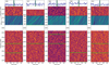 |
Fig. C.1 The same as Fig. 6 for B06-10. |
| In the text | |
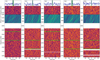 |
Fig. C.2 The same as Fig. 6 for B11-15. |
| In the text | |
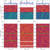 |
Fig. C.3 The same as Fig. 6 for B16-18. |
| In the text | |
Current usage metrics show cumulative count of Article Views (full-text article views including HTML views, PDF and ePub downloads, according to the available data) and Abstracts Views on Vision4Press platform.
Data correspond to usage on the plateform after 2015. The current usage metrics is available 48-96 hours after online publication and is updated daily on week days.
Initial download of the metrics may take a while.