| Issue |
A&A
Volume 690, October 2024
|
|
|---|---|---|
| Article Number | A319 | |
| Number of page(s) | 12 | |
| Section | Atomic, molecular, and nuclear data | |
| DOI | https://doi.org/10.1051/0004-6361/202450588 | |
| Published online | 18 October 2024 | |
The quantum yield of O(1S) in CO2 photolysis retrieved from the Martian atmosphere
The quantum yield of O(1S) in CO2 photolysis
1
Ludwig Maximilian University, Faculty of Physics, University Observatory,
Scheinerstrasse 1,
Munich
81679, Germany
Corresponding author; This email address is being protected from spambots. You need JavaScript enabled to view it.
2
ARTORG Center for Biomedical Engineering Research, University of Bern,
Murtenstrasse 50,
3008
Bern, Switzerland
3
University College London, Department of Physics & Astronomy,
Gower St,
London
WC1E 6BT, UK
4
University of Warwick, Department of Physics, Astronomy & Astrophysics Group,
Coventry
CV4 7AL, UK
Received:
2
May
2024
Accepted:
5
September
2024
Abstract
Photochemistry studies the interactions between light and molecules. Ultraviolet radiation interacts with the atmosphere, and due to its energy, it can dissociate, excite, or ionize its constituents, which initiate other processes. A good knowledge of the interaction between photons of different energies with molecules and atoms is crucial for accurately modeling the atmospheric physics and for climate predictions. Despite its importance, photo-fragment dynamics lacks data because the experimental setup is difficult. We used the upper Martian atmosphere as a natural laboratory to measure the quantum yield O(1S) from CO2 + hv as a function of wavelength. We analyzed 4 years of continuous remote-sensing observations from the NASA MAVEN/IUVS spectrograph within a Bayesian framework analysis tool. We retrieved the quantum yield for the first time through its entire production spectral range, ≈80–126 nm, and achieved uncertainty from 10% to 20% on average. While at Lyman-α (121.6 nm), we achieved a precision of 2% by taking advantage of the properties of the upper Martian atmosphere.
Key words: atomic data / atomic processes / molecular data / Sun: UV radiation / planets and satellites: atmospheres / ultraviolet: planetary systems
© The Authors 2024
 Open Access article, published by EDP Sciences, under the terms of the Creative Commons Attribution License (https://creativecommons.org/licenses/by/4.0), which permits unrestricted use, distribution, and reproduction in any medium, provided the original work is properly cited.
This article is published in open access under the Subscribe to Open model. This email address is being protected from spambots. You need JavaScript enabled to view it. to support open access publication.
1 Introduction
Atmospheric chemistry is one of the fundamental physical processes that shape the evolution and climate of planetary atmospheres and eventually plays a crucial role in the emergence and maintenance of life. In most of the planets, the chemistry is driven by the interaction of the atmosphere with the space environment, both with the stellar wind and incoming radiation. While energetic particles interact high up in the atmospheric layers, the exact height depends on whether the atmosphere is shielded by a magnetic field. The energetic part of the radiation spectrum (<250 nm) will penetrate deeper, down to 50–60 km in the Martian atmosphere, and causes photodissociation or photoionization. This interaction causes disequilibrium in the atmosphere and initiates chemical reactions that lead to what we describe as photochemistry. In a more expansive context, our comprehension, derived from laboratory experiments, that assists in explaining atmospheric phenomena, primarily centers on the accessible chemical pathways involved in photodissociation processes, the quantum efficiencies linked to these pathways, and how these quantum efficiencies are influenced by the wavelength of the photolysis. Nonetheless, it is clear that the way in which energy is distributed among the fragments and their chemical composition can significantly impact various aspects of atmospheric chemistry. Undoubtedly, electronic excitation plays a crucial role in altering chemical reactivity, and the emissions originating from electronically excited states contribute to the airglow observed in the atmospheres of numerous planets. These airglow emissions frequently offer valuable insights into the underlying chemistry at work and are used as tracers of atmospheric dynamics and other physical processes (e.g., Gérard et al. 2019b,a; Ritter et al. 2019; Gkouvelis et al. 2020b,a). Moreover, quantum yields (Φ(λ)) of photolysis rates are the basis of photochemical modeling in a wide range of scientific topics. Φ(λ) measurements use a variety of techniques that usually involve a narrow energetic beam of light that is able to photolyze the molecule and a detector aimed to receive secondary radiation from the photofragments that end up emitting photons from de-excitations. These secondary products stay in the excited state long enough that a large port of them collide with the chamber walls, resulting in de-excitation without emitting a photon. The fraction can vary significantly depending on several factors, including the type of atom, the conditions of the experiment, the material, and the temperature of the chamber walls. This can cause large uncertainties in the measurement. For the forbidden oxygen transitions, the quenched fraction can reach up to 50% (Lawrence 1972b; Slanger & Black 1978). Furthermore, Φ(λ) strongly depends on the energy of the photon, with efficiency changes across wavelengths from 100% to 0.1% that cause the signal to the detector to vary from very faint to a saturation level. These laboratory experiments require expensive and sophisticated instruments, but still have large uncertainties. The expansion of atmospheric sciences, climate studies, planetary systems, exoplanet research, and related fields, which require precise data for an accurate modeling and predictions, is driving the demand for more and better measurements in fundamental atomic and molecular properties, such as photofragment dynamics.
In this work, we focus on CO2 photolysis photofragments, and more specifically, on the portion that leads to atomic oxygen in the 1S excited state. We show that instead of creating the laboratory environment for measuring CO2 photofragments, we used the middle to upper atmosphere of Mars (70–180 km above surface) as a natural laboratory to retrieve the most precise Φ(λ) as a function of wavelength.
As we demonstrate, the literature on the photodissociation dynamics of carbon dioxide is considerable poorer than for other molecules, for example, ozone, even though it is a relatively uncomplicated triatomic molecule and has a fundamental importance in our understanding of the chemistry that occurs in planets, whose atmospheres are based on it.
The lower Martian thermosphere, ≈120 km, has the same composition as the bulk atmosphere (Fox & Dalgarno 1979; Fox & Bougher 1991), which consists of more than 95% CO2. Photodissociation of CO2 already acts from the homopause, ≈80 km, and in combination with diffusion to the gravitational field causes the products of photolysis (CO and O) to become relatively more abundant (Fox & Sung 2001; Fox & Dalgarno 1981; Fox & Bougher 1991; Gronoff et al. 2008; Simon et al. 2009; Gronoff et al. 2012). The main oxygen channels of CO2 photolysis products, which are of interest of this work, are summarized in Sect. 2. The metastable 1S and 1D excited states of atomic oxygen lie 1.98 and 4.19 eV, respectively, above the ground 3P state. The O(1S) decays to the O(1D) by emitting a green line at 557.7 nm. The transition from O(1D) to O(3P) produces red doublet (630 and 636.4 nm) lines, and the emission we are interested here extends from 1S to 3P, which leads to the ultraviolet 297.2 nm spectral line. O(1S) and O(1D) have a lifetime of 0.8 and 110 seconds, respectively (Baluja & Zeippen 1988; Froese Fischer & Tachiev 2004). The thresholds of O(1S) and O(1D) production in dissociative excitation of CO2 are 128.6 and 167.1 nm, respectively (Huebner et al. 1992). Photodissociative (PD) excitation of CO2 is the main production mechanism of O(1S) in the dayglow of Mars and Venus (Fox & Dalgarno 1979; Gkouvelis et al. 2018).
The photodissociative yield of O(1S) from CO2 was measured in various works, all in the 1970s (Lawrence 1972b; Koyano et al. 1975; Slanger et al. 1977; Bibinov et al. 1979). These measurements are plotted together in Fig. 1 with the uncertainty proposed from each work. Each of the laboratory measurements covers part of the spectral range where the O(1S) production channel is open, and the measurements were made in different resolutions. Slanger et al. (1977) conducted experiments to measure the quantum yield of O(1S) within the 106–117 nm wavelength range. Their findings revealed that the yield was consistently one between 110 and 115 nm. However, they observed a sharp decrease in yield to lower than 0.15% below 110 nm, at 108.9 nm, corresponding to a strong Rydberg transition in CO2. Slanger et al. (1977) emphasized that the maximum yield of O(1S) at 108.9 nm could not exceed 0.2%, and the minimum might even be zero. Lawrence (1972b) also measured the yield across wavelengths from 81 to 121.6 nm. In this range, the yield was consistently one between 108 and 115 nm. However, these measurements did not show a sudden drop around 108.9 nm. This discrepancy may have been due to the narrow absorption feature at 108.9 nm, which might have gone undetected in the Lawrence (1972b) measurements, which were conducted at a lower resolution of 0.8 nm. Bibinov et al. (1979) extended the measurement of the quantum yield within the wavelength range of 102–128 nm. They reported a nonzero O(1S) yield for wavelengths up to 128.6 nm, but their measurements beyond 115 nm were less reliable, with an estimated uncertainty of 50% according to the authors.
Especially the measurement of the O(1S) yield at 121.6 nm is challenging due to the very low absorption coefficient of CO2. At 121.6 nm lies the Lyman-a line, and special attention is given to this line. The accepted value by the community that uses these data comes from Lawrence (1972b), who measured a yield of 13% at this wavelength. Ly-α almost solely determines the magnitude of the O(1S) production at altitudes below 100 km in the Martian atmosphere and below 120 km at Venus (Fox & Dalgarno 1979; Simon et al. 2009; Gronoff et al. 2012; Gkouvelis et al. 2018).
For the Φ(λ) of the O(1D) channel, laboratory measurements are more challenging. There is no direct measurement of the O(1D) yield in photodissociation of CO2 because the long lifetime (110 s) makes it difficult to measure in the laboratory. Slanger & Black (1978) studied CO2 photolysis at wavelengths below 167 nm and concluded that the total photodissociation yield of CO2 is unity between 106.7 and 167 nm. Using an indirect method, they estimated that O(1D) would be the primary product in the photodissociation of CO2 between 125 and 167 nm with a unit yield. Below 125 nm, the O(1D) yield decreases because another photodissociation channel opens (O(1S) + CO(X)). Between 115 and 110 nm, the O(1D) yield becomes zero since the O(1S) yield is one in this region. Below 110 nm, the O(1D) + CO(X) channel opens up again with an O(1D) yield of 0.65 ± 0.1. At 108.9 nm, where the O(1S) yield is suddenly reduced (to lower than 0.15), Slanger et al. (1977) suggested that the O(1D) yield can reach a maximum value of one. Slanger & Black (1978) also noted that at 106.7 nm, the O(1S) and O(1D) yields would be 0.6 and 0.35, respectively, with a value of 0.05 for the CO(α3Π) yield (Lawrence 1972a).
We summarize the quantum yields of excited photofragments in the CO2 photolysis in the lower part of Fig. 2. These values are presented without error estimates and are the values accepted by the scientific community, at least used widely for atmospheric modeling of planetary atmospheres (Huestis et al. 2010). From all the information mentioned above, it is evident that Φ(λ) of the 1S and lD channels are connected to each other, since the latter is mainly an indirect estimate based on the first. 1S has very large uncertainties across its entire spectral range, however.
The Martian atmosphere produces a unique environment for the observation and study of the metastable oxygen lines. It is mainly composed of CO2. In the upper mesosphere – lower thermosphère, higher than 60 km, the densities are such that collisional quenching is negligible, at least for the O(1S) de-excitation and production of the ultraviolet 297.2 nm line. Moreover, we show that the attenuation of the solar UV spectrum, that is, Fig. 4, in combination with the solar cycle and Martian atmospheric variability can provide us with enough information to extract the O(1S) quantum yield from CO2 photolysis.
In summary, our method is based on two important factors. The first factor is the simplicity of the fundamental physics that produce the forbidden atomic oxygen transition from 0(1S) to the ground state, O(3P), which occurs in the upper atmosphere of Mars. The second factor is the enormous number of remote-sensing observations from the Imaging Ultraviolet Spectrograph (IUVS) on board the Mars Atmosphere and Volatile Evolution (MAVEN) orbiter (hundreds of thousands of spectra) we have at our disposition. With the combination of these two factors, we can solve the inverse problem to analyze the observational data in order to retrieve the quantum yield of CO2 + hv into O(1S), spanning the wavelength range homogeneously from 80 to 130 nm.
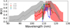 |
Fig. 1 Summary of the published laboratory results for the quantum yield, Φ(λ). The actual measurements are represented by dots, and the uncertainty is shown by the shadowed area, except for S1977 and K1975, for which we plot no errors for clarity. Their error values are about 15–30%. L1972: Lawrence (1972b), B1979: Bibinov et al. (1979), S1977: Slanger et al. (1977), K1975: Koyano et al. (1975). |
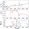 |
Fig. 2 Range of spectral interest. Top and middle: same as Fig. 3, but zoomed in the Φ(λ) spectral region. Bottom: Φ(λ) as adopted by Huestis et al. (2010) based on all laboratory measurements that are shown in Fig. 1. The uncertainties of the proposed values are shown in Fig. 7. |
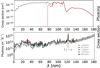 |
Fig. 3 Solar input spectra. Top: photo-absorption cross section of CO2 at 250 K as the gray line. Overplotted as the dashed red line is the photodissociation cross section. For shorter wavelengths of the spectrum, the photoionizing energies have a threshold ≈80 nm. Bottom: Typical solar EUV/UV spectrum at 1 nm resolution, as observed by the MAVEN/EUM spectrograph, scaled at 1 AU, at different dates of the solar cycle. |
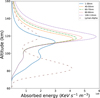 |
Fig. 4 Typical photon penetration and energy deposition for a variety of spectral bands. The shape and intensity of each wavelength depend on the vertical distribution and variability of CO2 in the solar spectrum. |
2 Approach
We based our method on the combination of three basic components.
Modern remote-sensing observations. The NASA MAVEN satellite that orbits Mars simultaneously observes the solar XUV spectrum and far-/mid-UV from the Martian airglow.
The observed 297.2 nm emission line is solely produced from O(1S) → O(3P) + hv(297.2nm) and the O(1S) is ≈100% produced by CO2 photodissociation at altitudes lower than 100 km and ~90 to 95% at higher altitudes.
The conditions in the Martian thermosphère are such that collisional quenching is practically absent (the loss frequency due to quenching is always lower than the photon emission relaxation; see, e.g., Raghuram et al. 2021) and the O(1S) state has enough time to de-excite through photon emission.
These three components can be combined in a Bayesian analysis framework (see Appendix B), so that by fitting a forward model (see Appendix A) to the observations, we can retrieve two quantities. One quantity is the vertical distribution of the CO2 density, and the other quantity is the quantum yield (Φ(λ)) as a function of wavelength. The CO2 density profile presents seasonal and diurnal variations. Φ(λ), in contrast, is expected to have a time-independent function.
Photolysis of the CO2 molecule can lead to the following products of CO(X) + O(Y), where X and Y are different states of CO and O. Focusing on the oxygen fragments, we can write
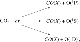
where 3P is the fundamental atomic oxygen state, and 1D and 1S are excited states whose transitions to lower energetic levels lead to emission of photons, or they can be deactivated through quenching (collisional deactivation). The 1D →3P transition leads to the so-called optical green line at 557.7 nm wavelength. The 1S can transition either directly as 1S →3P, which is the 0297.2 nm or through two-step emission 1S →1D →3P (see Fig. 5). The first step is the oxygen red line at 630 nm. These metastable atomic oxygen transitions cause the thin dayglow layer in the upper atmosphere of Earth at ≈90 km (Zhang & Shepherd 2005; Witasse et al. 1999) and the polar aurora. The optical red and green lines were recently discovered on another planetary body, Mars (Gérard et al. 2021, 2020). The ultraviolet 297.2 nm line was first detected in the Martian atmosphere with the ultraviolet spectrometer during the Mariner 6 and 7 flybys (Barth et al. 1971; Stewart 1972), but its detailed vertical profile was revealed only few years before by the IUVS instrument (McClintock et al. 2015) on board the MAVEN Mars orbiter. It presents a double peak, one peak at about 120 km, and another deeper peak at 70–80 km that is much stronger. This double peak is the result of two factors. A minimum in the CO2 photoabsorption cross section at about 121 nm and of the Lyman-α solar emission line at the same wavelength that is two orders of magnitude stronger than the background energy spectrum (Fig. 3). This causes Lyman-α to become absorbed deeper in the CO2 atmosphere and accordingly, to produce photofragments. This double-peak structure was predicted for the Martian atmosphere by Fox & Dalgarno (1979), but its detailed structure and the seasonal variation presented in the observations was explained by Gkouvelis et al. (2018). They performed direct forward Monte Carlo (DFMC) simulations to account for all sources and sinks of the O(1S)) excited state in order to calculate the vertical emission in the oxygen UV 297.2 nm line. The main conclusion about the production of this line is that it is mainly generated by photodissociation of CO2 (Fig. 6). Later studies agreed with these results (Raghuram et al. 2021; Evans et al. 2023; Aoki et al. 2022; Gérard et al. 2021; Soret et al. 2023).
In order to model the observations, we neglected any other minor sources (orders of magnitude lower) and concentrated on the CO2 photolysis products. It follows that the photons contributing to the O297.2 nm line per altitude in the vertical grid can be calculated as
![Mathematical equation: $\matrix{ \hfill {\eta {{(297.2nm)}_z} = {P_z}\left[ {{\rm{O}}\left( {^1{\rm{S}}} \right)} \right]{{{A_{297.2}}} \over {{A_{Total}}}}} \cr \hfill { \times \left[ {{A_{Total}} + {K_{{\rm{C}}{{\rm{O}}_2}}}\left( {{A_{Total}} + {K_{{\rm{C}}{{\rm{O}}_2}}}{{\left[ {{\rm{C}}{{\rm{O}}_2}} \right]}_z} + {K_{\rm{O}}}{{[{\rm{O}}]}_z}} \right.} \right.} \cr \hfill {\left. {\left. { + {K_{{\rm{CO}}}}{{[{\rm{CO}}]}_z}} \right)} \right],} \cr } $](/articles/aa/full_html/2024/10/aa50588-24/aa50588-24-eq1.png) (1)
(1)
where Pz[O(1S)] is the total volume production rate of O(1S) atoms at each altitude z, and ATotal is the sum A297.2 nm + A557.7 nm of the transition probabilities of the O(1S) → O(3P) and O(1S) → O(1D) transitions. The branching ratio of the two transitions was modeled from quantum mechanics ab initio principles (NIST; Kramida et al. 2018) and measured from remote-sensing spectroscopic observations (Gérard et al. 2020). They both agree to a value of A555.7 nm/A297.2 nm = 16.7. K are the quenching coefficients for CO2, O, and CO. We adopted the values  cm3/s, KCO = 7.4 × 10⁻¹⁴exp(−957/r)cm3/s from Capetanakis et al. (1993), and KO < 1.2 × 10⁻¹⁴cm3/s from Krauss & Neumann (1975) and Slanger & Black (1981). The total transition probability from the 1S state is 1.34 s. The deactivation through collisional quenching in the Martian atmosphere becomes important below 70 km. The total production rate of oxygen atoms in the 1S state can be written as
![Mathematical equation: $P{\left[ {{\rm{O}}\left( {^1{\rm{S}}} \right)} \right]_z} = {\left[ {{\rm{C}}{{\rm{O}}_2}} \right]_z} \times \mathop \smallint \nolimits^ _{{\lambda _a}}^{{\lambda _b}}{\sigma _\lambda }{{\rm{\Phi }}_\lambda }{I_{\lambda ,z}}d\lambda ,$](/articles/aa/full_html/2024/10/aa50588-24/aa50588-24-eq3.png) (2)
(2)
where [CO2]z is the CO2 number density at z altitude, σλ is the total photoabsorption cross section, Φλ is the quantum yield to the 1S state from the CO2 photolysis, and Iλ,z is the attenuated solar spectrum as
 (3)
(3)
Here,  is the solar spectrum at the top of the atmosphere (TOA), which is directly observed by the EUVM spectrograph on board MAVEN (Eparvier et al. 2015), and τ is the optical depth. One final step in order to be able to directly fit the observations is to account for the line-of-sight integration considering the limb geometry of the observation (see Sect. 2.1).
We used the above simple modeling approach with the given input parameters of the time of the observations, which we can write as y, to be described as F(x). x are the parameters of the model that are not well constructed and produce discrepancies in the fit of the observation to the model. We then inverted the problem by means of iterations to retrieve the lesser known parameters with confidence and account for all errors involved in the process. For our specific problem, the vertical distribution of the CO2 number density and the Φ(λ) quantum yield are the parameters that we considered to be free and that we retrieved. The CO2 number density and its variation is an important parameter for the climatology of the middle and upper Martian atmosphere. However, this is beyond the scope of this work, which is focused on determining Φ(λ) at all wavelengths, which is nonzero and is a novel approach for the estimation of these molecular/atomic properties, which so far were purely measured in laboratories.
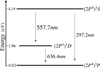 |
Fig. 5 Oxygen energy configuration of the 2P4 state. The three emission lines are a product of the population at the levels 1S and 1D. |
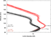 |
Fig. 6 Typical constructed vertical oxygen 297.2 nm scans as observed from MAVEN/IUVS. The mean solar zenith angle is indicated as 〈SZA〉 for the two profiles, where red shows observations around orbit 970 and black shows observations around orbit 2483. |
2.1 Observations
2.1.1 MAVEN/IUVS
The IUVS is one of the eight scientific instruments on board the MAVEN satellite, which is in Mars orbit since October 2014. By now, more than 8 years of quasi-continuous airglow observations from IUVS are publicly available. It has collected data for more than 20 000 orbits, including hundreds of thousands of vertical limb scans. It supports two spectroscopic modes, using two separate gratings that provide the required resolving powers. One of the two modes operates near normal incidence and covers the 110–340 nm range with a resolving power of 250. The second mode uses a prism cross-disperser and an echelle grating to cover the 120–131 nm range. IUVS is operated in five different observation modes: stellar occultation, atmospheric limb scans, echelle, disk mapping, and Martian corona observations. This project only focuses on the limb-scan observations and only uses normal incidence spectroscopy, which is divided into two channels, the far-UV (FUV) and the mid-UV (MUV). The ultraviolet light is dispersed by the grating into the above two diffraction orders. Finally, the light passes through the entrance slit with a 0.06 deg ×11 deg field of view and reaches the detector. The emission of interest here is detected in the MUV channel with a spectral resolution of 1.2 nm and a dispersion of 7.27 nm/mm. The noise sources are photon-counting noise, detector dark current noise, quantization noise, intensifier excess noise, and detector read-out noise (McClintock et al. 2015).
The calibration of the spectra is based on ground tests as well as in-flight measurements using UV-bright stellar targets with well-known spectral fluxes. For the MUV channel, the systematic uncertainties are estimated to be about 25% (Jain et al. 2015; Schneider et al. 2015; Stevens et al. 2015). For this study, we applied a correction factor of 0.69 to the O297.2 nm absolute intensities, following the calibration revision made in November 2018 (Gkouvelis et al. 2018, see Sect. 2). More details of the instrument properties and the observation modes may be found in the instrument review publication McClintock et al. (2015). During periapsis observations, the altitude of the spacecraft is lower than 500 km. The observations were made with the detector looking in a direction almost parallel to the surface and the slit oriented horizontally. IUVS is equipped with a rotating mirror that allows 21 different positions, so that it can perform limb observations at different altitudes as it passes close to or inside the atmosphere. Therefore, each scan provides a limb profile of the different spectral features.
During each orbit, IUVS performs a maximum of 14 scans. However, two of the scans are in inbound and outbound mode, where the observing geometry cannot be used for our analysis. An example of multiple limb-scan observations is shown in Fig. 3. Level 1c data include the calibrated brightness of individual emissions that has been reduced by isolating emission features and spatial binning to facilitate processing: the dayglow spectra include many different atomic and molecular emissions, including the spectral feature from oxygen at 297.2 nm. Each emission may be identified by its wavelength and its expected relative intensity. The brightness of any atomic or molecular feature is determined by using a multiple linear regression method to fit the various components of each observed spectrum following convolution with the instrumental line spread function (Stevens et al. 2015; Gkouvelis et al. 2018). In addition to these atomic and molecular emissions, the fit templates also include a reflected solar spectrum component. This solar scattered-light component becomes important for limb observations with tangent point altitudes below about 100 km, especially in the longer-wavelength segment of the MUV spectra. In this region, reflection by high-altitude clouds and dust as well as stray light within the instrument can contribute to the background signal (Stevens et al. 2015; Schneider et al. 2015; Jain et al. 2015). For the IUVS output products, a high signal-to-noise ratio average solar spectrum was used, measured by the IUVS instrument, in the multiple linear regression analysis to calculate the brightness of various emissions provided in the level 1c data. The shape of this solar scattered-light component is an excellent estimate of the scattered light embedded in the airglow signal, and it efficiently removes the solar stray light at these altitudes. The altitude range of the observations varies in each scan, depending on the position of the spacecraft in its orbit at the time of the observation. We used the level 1C version 13 of the data. The data needed for this study can be downloaded from the NASA Planetary Data System (PDS)1 archives.
2.1.2 MAVEN/EUVM
The retrieval method requires an accurate solar energy source. This is a vital observational input because the ultraviolet solar energy reaches the upper Mars atmosphere and controls all the UV airglow emissions. The Extreme Ultraviolet Monitor (EUVM) spectrograph on board MAVEN is collecting solar energy in three bands, and based on these observations, a detailed spectrum was constructed with a resolution of 1 nm (Eparvier et al. 2015; Thiemann et al. 2017). The data are provided with a temporal resolution down to 1 minute as well as daily averages for the whole MAVEN observing period. We used the one-minute observations to construct average spectra that temporally correspond to the IUVS observations. We used the latest available version. This can vary from version 23 for the first years of the mission to version 1 for the most recent observations. These spectra were introduced into the forward model together with all the appropriate observational conditions. All data are available from PDS2.
2.1.3 Binning of the data
All the available datasets from PDS and PSA were downloaded in order to clean the nightside observations. We used data up to SZA = 80°. In order to retrieve the optimal atmospheric information from the data and to increase the signal-to-noise ratio, the observations were binned in groups of solar zenith angle and latitude in temporal space. For SZA, we binned them together in degrees 0–40 and then every 10 degrees. For the latitude, we binned every 10 degrees, and we used 1 sol per profile, which correspond to 4 orbits. The vertical resolution of the observations is 5 km. A quality control was performed for each bin/mean vertical profile based on the shape of the profile, and the emission in altitude is higher than 180 km, which is expected to be close to zero. The total uncertainties of the observations are given in Sect. 3. As an example, Fig. A.1 shows two vertical profiles that were constructed from a binning of vertical scans with 4 orbits each (1 sol) for two different solar longitudes. The overall IUVS data set includes observations from about 15 000 orbits, covering all ranges of latitudes, solar zenith angles, and solar longitudes. For this study, samples corresponding to various conditions can therefore be selected in order to create average limb profiles that were used to characterize the emission and its variations.
3 Analysis
We analyzed more than 20 000 spectra taken in a period of 4 years, ≈2 Martian years, and we constructed more than 2000 vertical profiles. Since the target was to retrieve Φ(λ) , which is expected to be a constant function of wavelength over all of the analysis, we chose to filter out incomplete vertical profiles in order to facilitate the analysis. By incomplete we mean that instead of constructing the vertical profiles as seen in Fig. A.1 only part of it was been able to be observed, only one peak or less. These partial observations where due to observing geometry or data reduction pipeline rejection due to the quality of the outcome product (McClintock et al. 2015; Jain et al. 2015). Approximately 70% of the constructed profiles were complete, covering 16 vertical grid points, and they had at least five vertical scans.
Every vertical profile was constructed for each sol (Martian day) as  with Δyi the random error from the detector. It follows that
  and Δ〈y〉 ≫ <σn , where <σn is the standard deviation of the mean. We assigned then <σn as the noise of the observations as it is found for each altitude layer. A typical mean profile with σn assigned as noise is shown in Fig. B.2a, where the shadowed gray area is the noise as σn, and the blue line curve indicates the mean vertical profile as constructed from all the scans that corresponds to a sol. In the same plot, we show the forward-model simulation of the vertical profile, using the a priori information, background atmosphere, and quantum yield as shown in Fig. 7 with the total uncertainty of all the parameters involved in the forward model in the shadowed red area. In a first approach, the agreement between the observations and the model is within 5–10% in terms of brightness and within 20% in terms of the vertical density profile, as was shown in previous studies (Gkouvelis et al. 2020b; Gérard et al. 2020). This is expected because all the physics are controlled with confidence. The remaining differences are due to the stochastic diurnal variations of the CO2 vertical number densities and to our poor knowledge of the quantum yield laboratory measurements, which is a sensitive factor in these processes. Fig. B.2b shows a typical difference of the first guess, a priori, for the CO2 vertical number densities, and the final output is shown and differences in percentage are plotted in Fig. B.2c.
The final result of the Φ(λ) in comparison with the currently accepted values is shown in Fig. 7 with red dots. The resolution is 1 nm, and this is bound to the solar spectrum resolution. The error bars are plotted for each point and vary significantly for various wavelengths. The errors are calculated as
 (4)
(4)
where ϵnoise is the noise error covariance matrix, and ϵi is the standard deviation of all the retrieved Φ(λ) profiles and is calculated as
 (5)
(5)
where N is the total number of retrievals,  is the mean profile, and Wi is the weight of each individual profile, which is an indicator of how many vertical profiles were used to construct it per sol.
Error evaluation. Special attention was given to the propagation of the uncertainties on the final products, CO2 profiles, and Φ(λ) from all the errors involved in the analysis pipeline, both from the forward model and the observational data. For the forward model, the general propagation equation used is
 (6)
(6)
where F(p) is the forward model depending on the p parameters, and pi is the uncertainty of each individual parameter.
All the parameters involved are given in Table 1, which summarizes the path of the error analysis to the total uncertainty propagation. We have three types of errors in this work: Obs. comes directly from the observational measurements and was given together with the processed data. FM is the propagation of errors within the forward model. Output is the uncertainties of our output products.
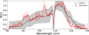 |
Fig. 7 Retrieved Φ(λ) against proposed curve from Huestis et al. (2010) with the uncertainties involved as a function of wavelength. The shaded gray area is a simplified 1er error estimate combining all previous works. |
Error magnitude of various parameters in our analysis pipeline.
4 Discussion
We have analyzed hundreds of thousands of ultraviolet spectra, constructing vertical limb profiles of the O297.2 nm dayglow emission line of the middle and upper Martian atmosphere. The physical conditions of the Martian atmosphere are ideal for observations of metastable oxygen transitions, especially from the O(1S) excited state, because due to the low pressure, the maximum quenching effect is smaller than 5% at 60 km and vanishes exponentially upward. Our high confidence of understanding the physical processes that produce the O297.2 nm emission in combination with the observational data of the solar input spectrum at the top of the atmosphere can enable the solution of the inverse problem. We retrieved the quantum yield,Φ(λ), of O(1S) from the photolysis of CO2 at all the producing wavelengths, ~80–128 nm. This is the first time that a quantum yield was retrieved using remote-sensing observations. We confined the uncertainty to lower than 20% and even to 2% for various channels. The differences occur within the combination of two main factors. First, the dependence of the O(1S) production at a given channel overlaps with other channels, so that it is uncertain which channels contribute to the observed profile, and the variability of the CO2 column distribution in combination with the solar spectrum did not give us sufficient information. Conversely, the channels that we are able to retrieve more precisely are the vertical domains, in which we can have high feedback. As an example, the Lyman-a line almost solely produces the lower peak, which is typically brighter than the upper peak by ≈2.5 times. This mechanism of one wavelength, Lyman-α, and one absorber, CO2, is similar to the so-called Chapman function , which explains the rate of photoionization in planetary atmospheres (Chapman 1931). This combination of a strong signal and monocromaticity make this specific channel our best measurement with 1σ down to 2%.
The overall spectral structure of the retrieved quantum yield agrees well with previous laboratory measurements in the 1960s and 1970s. There are three main differences: The first two differences are the two peaks, which are present around 90–95 nm and 105 nm. The third difference is the Lyman-α line, for which we are able to retrieve the value Φ(121.6) = 0.09 ± 2%. This disagrees with our previous semi-empirically constructed value 0.075 (Gkouvelis et al. 2018) and was used by various groups (Raghuram et al. 2021; Aoki et al. 2022; Evans et al. 2023). The two peaks are both present in a region in which various wavelengths overlap, and the variation in minor production mechanisms of O(1S)) might be a source of error. In contrast, the Lyman-a region was retrieved from wavelengths that penetrate deep into the atmosphere, where the signal is bright and secondary production sources are negligible, and we therefore consider the retrieved value to be robust.
Method limitations and future improvement strategies. We described above that in order to gain feedback information about Φ(λ), a combination of strong solar radiation and the difference in the cross-section between channels is required, so that we can catch different wavelengths in the vertical domain. The cross-section will essentially be the same within the small temperature variation that we considered in the Martian thermosphere. The overlapping cross-sections gives us less information. Nevertheless, having observations from 5 years, almost half a solar cycle, our solar input spectrum will change so that we can gain information about the shape of the solar spectrum. Especially in short periods in which solar flares occurred (e.g., Jain et al. 2018), the shape of the solar spectrum shows the strongest change, and thus, we can gain valuable information by adding this information to our analysis scheme.
A key assumption of this method is that Mars mainly has a CO2 dominated atmosphere. This assumption is valid up to ≈150 km. Even starting from ≈120 km the photodissociation starts playing an important role. In the composition of the neutral atmosphere, the CO2 mixing ratio decreases with altitude. However, other species do not introduce additional O(1S) production or loss mechanisms. Instead, the error is introduced when the attenuation of the solar spectrum is calculated. In order to achieve more precise results, in situ measurements of the background atmosphere have to be adopted simultaneously with the observations of this work. It is possible that these measurements exist from the MAVEN deep-dip mass-spectroscopy experiment. These deep dips are spacecraft aerobraking maneuvers in which the orbital distance from the surface of the planet can reach 100 km of altitude (Bougher et al. (2015); Mahaffy et al. (2015)). For wavelengths higher than Lyman-a, the errors increase to 20%, while the mean value goes to zero. These wavelengths penetrate deepest into the Martian mesosphere, and the detected signal is weak. Furthermore, in the reduction of IUVS data, the solar scattered-light removal might cause an overcorrection in the treatment of the data. Even though our results agree with previous works on these wavelengths, we note that the values should be considered as low confidence.
Our results have consequences for future studies of the middle Martian atmosphere climatology retrieval processes that are based on the airglow emissions of oxygen metastable states that use these emissions as proxies of atmospheric property variations. Furthermore, in the new era of precise exoplanetary spectroscopy and the necessity of good knowledge of chemical reactions and a standard base of comparison between models, quantum yield libraries can be used to minimize our errors in the modeling and interpretation of distant worlds.
Acknowledgements
L.G. would like to thank Prof. Jean-Claude Gérard for the insightfull discussions on airglow emissions and the literature of experimental measurements. The authors would like to thank the Theoretical astrophysics for extrasolar planets Munich chair members for their comments on this work.
Appendix A Forward model
The forward model plays a vital role in every inversion process. When it comes to extracting atmospheric parameters from air-glow observations, it is crucial to replicate the observations with a high degree of confidence in the underlying physical mechanisms. To support this endeavor, we employed a comprehensive photochemical model designed for airglow emissions analysis. our model has previously been successfully applied to analyze various emissions, including the UV emissions of O(1S)) at 297.2 nm, the  UV doublet, and the newly discovered green and red optical emission lines on Mars as documented in Gkouvelis et al. (2018), Gérard et al. (2019b), Gérard et al. (2020), Gérard et al. (2021) and Soret et al. (2022). In Fig. A.1, a simulation is showing all the production mechanisms of the O(1S)) for a snapshot of time at the Martian atmosphere. It follows that all the sources can be neglected and only photodissociation can be taken into account. We can then construct our forward model for this work based on Eqs. (1) to (3). Where the inputs needed are the cross sections, solar spectrum, the background atmosphere and the geometry of the observation.
Total photo-absorption cross-sections was taken from Venot et al. (2018) for CO2 and the proposed parametrizations for temperature dependence were adopted accordingly and Rayleigh scattering is accounted for in the appropriate wavelengths. For other molecules total photo-absorption cross sections were taken from Heays et al. (2017) and references therein. Spherical geometry is assumed with an onion pealing layers for the calculation of the optical depth path of each wavelength when the sun is at solar zenith angle χ given as
 (A.1)
(A.1)
where nz is the number density of the atmosphere within a layers of altitude z′ and z′ + Δz’.σλ the cross section and ds is the length that the beam of light travel between the layers with an incident angle χ′. It follows that
 (A.2)
(A.2)
where R is the radius of the planet, z is the studied altitude at each step, z′ and z′ + Δz′ are the outer limits of the layer the light travel ds length. This adoption enables us to avoid the parallel plane approximation and be able to include observational data up to 80o degrees of SZA.
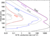 |
Fig. A.1 O(1S)) production mechanisms in the Martian middle and upper atmosphere. Photo-dissociation is responsible for 97% of the production for altitudes higher than 100km as have been calculated using direct forward Monte Carlo simulations described by Gkouvelis et al. (2018) and Shematovich et al. (2008). |
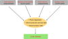 |
Fig. A.2 Synopsis of the forward model calculating the limb intensity profiles imitating the observation geometry of the measurements. |
While we model the production and emission rate at the vertical grid, in order to directly compare with the observation at vertical limb scans we have to account for the line-of-sight integration. The detector is measuring photons not only from the vertical domain we consider, but instead across the line of sight of each vertical tangent point have to be considered. The abscissa r along the horizontal line of sight is calculated as
 (A.3)
(A.3)
This will provide direct comparable units and geometry to the observations. Multiplication by a factor of 2 is due to symmetry along the line of sight with respect to the tangent point. This symmetric assumption is valid for the following reasoning. Since the most important contribution to the intensity is the tangent point and the layers very close to it. The tangent point is always from 100 to 200km away from MAVEN. The periapsis of the spacecraft was ≈ 175km for those observations. All our vertical profiles are approaching zero brightness above 150km. Observational campaigns that MAVEN went in ‘deep-dip’ mode were not used in this work.
While calculating limb intensity it is assumed that the emission rate is constant along local longitude/latitude. For the emission line considered in the this work the effect of absorption in the atmosphere is found to be negligible. A simplified flow chart of the forward model is given in Fig. A.2
Appendix B Inversion problem
In order to derive atmospheric quantities from remote sensing observations we have to invert the so-called forward problem. Our limb scan observations can be written as y with m dimensions, which are the vertical grid in altitude defined by the data. Given that we have confident physical understanding of the processes producing y we can write
 (B.1)
(B.1)
where F(x) represents a non-linear function that describes the physical processes, or in other words, the forward model that fits the observations. the inverse solution can then be found as
 (B.2)
(B.2)
The approach to the inversion problem in atmospheric physics is well described by Rodgers (2000) and have been widely used for planetary atmospheres of the solar system. A few successful examples of retrievals of atmospheric abundances are given by Grassi et al. (2005), Jurado-Navarro et al. (2015), and Jiménez-Monferrer et al. (2021).
The forward model can be linearized by accounting for a reference state, xo, and include a term that accounts for all the uncertainties involved in the instrument, ϵ . Equation (B.1) then becomes
 (B.3)
(B.3)
where the K is the Jacobian matrix which describes the sensitivity of the measurements in regards to changes of a given parameter in the forward model:
 (B.4)
(B.4)
An example of the Jacobian kernels in our retrieval process is shown in B.1. Given the non-linearity of the above equations, the solution to the problem is given numerically by an iteration process, following Rodgers (2000), von Clarmann et al. (2003), and von Clarmann & Glatthor (2019):
![Mathematical equation: ${{\bf{x}}_{{\bf{i}} + 1}} = {{\bf{x}}_{\bf{i}}} + {\left[ {{K^T}S_y^{ - 1}K} \right]^{ - 1}} \times \left[ {{K^T}S_y^{ - 1}({\bf{y}} - F({\bf{x}}))} \right],$](/articles/aa/full_html/2024/10/aa50588-24/aa50588-24-eq28.png) (B.5)
(B.5)
where y is the vector of limb observed measurements given at a grid of certain altitudes with dimension m which are the tangent heights where the observations are available. x are the retrieved parameters, in this case are the CO2 abundances within the altitude range of ≈70–150km and the Quantum Yield, Φ, across 80-130nm spectral range. F(x) is the non-linear function that represents the photochemical model solution to the airglow emission of the 297.2nm ultraviolet line. For a reasonable solution of the state vector, some a priori information, xα , is required. The inverse problem is usually an ill-posed problem, and its solution is very sensitive to noise propagation. Therefore, a smoothing constraint is included by means of a 1st-order Tikhonov reg-ularization matrix, R, which ensured independence from the a priori absolute values. The a priori absolute values in the form of vertical composition and temperature atmospheric input, as first guess, adapted to the time and location of the IUVS limb measurements will be obtained from a public database dependent on a global climate model (Forget et al. 2009; Millour et al. 2015; González-Galindo et al. 2005, 2015).
Finally, to avoid problems with strong non-linearities during the iteration process, a Levenberg-Marquardt (LM) damping (Levenberg 1944; Marquardt 1963) is used, following the same method described in von Clarmann et al. (2003). Considering all these terms, the solution to the inverse method is given by
![Mathematical equation: ${{\bf{x}}_{i + 1}} = {{\bf{x}}_i} + {\left[ {{K^T}S_y^{ - 1}K + R + \lambda I} \right]^{ - 1}} \times \left[ {{K^T}S_y^{ - 1}({\bf{y}} - F({\bf{x}})) - R\left( {{x_i} - {{\bf{x}}_{\bf{\alpha }}}} \right)} \right],$](/articles/aa/full_html/2024/10/aa50588-24/aa50588-24-eq29.png) (B.6)
(B.6)
where λ is the Levenberg-Marquardt damping factor, which is forced to be zero in the last iteration.
Equation (B.6) is iteratively solved starting from an initial guess and using spectra and Jacobians calculated by the forward model. The measurement covariance matrix was calculated from the noise-equivalent spectral radiance of the measurements. Convergence is reached when the change of the retrieval parameters with respect to the previous iteration becomes smaller than a given fraction of the retrieval noise error (60%). The main outputs are the quantum yield, CO2 number density and diagnostics, such as the averaging kernels, the noise error covariance matrix of the vertical resolution.
The retrieval scheme is broken down into four steps:
The a priori information on the background atmosphere was introduced in the forward model.
The forward model calculates radiances and the Jacobians, i.e the derivatives of the radiances with respect to the retrieval parameters.
The simulated profiles are passed into the retrieval control algorithm for iteration.
If the result does not satisfy the convergence criterion, the result is sent back to the forward model for recalculation, otherwise the retrieved profile has been obtained. The convergence is reached if the residuals are within a fraction of the measurements noise. By construction (see Sect. 2.1.3) all of the profiles were converged. We only include complete vertical profiles into the retrieval process. If a profile is incomplete or has fewer than five vertical scans, we removed it from the analysis. From the complete dataset, this was about 20% of the observations.
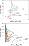 |
Fig. B.1 Typical Jacobian kernels. Top: Sensitivity of the forward model in the vertical distribution of CO2 number density. The different colours correspond to each altitude bin that is defined by the observational measurements. Bottom: Sensitivity of the quantum yield to the corresponding altitude grid. Different colours correspond to different wavelengths with lnm resolution from 80 to 128nm. With dashed black line we show the Ly – α line divided by a factor of 10. It is not surprising that Ly – α shows this sensitivity, since the production of the lower peak is almost solely produced by it. |
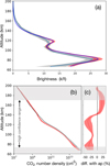 |
Fig. B.2 Demonstration of the algorithm in a case study profile from IUVS observations is shown as the light blue line and the data uncertainty is the grey shading, in panel (a) together with the forward model simulation using the a priori CO2 vertical density together with the total model uncertainty in shaded red. (b) The CO2 number densities: the black dashed line represents the a priori, the dashed red the final vertical distribution of CO2 number density where the fit satisfies the algorithm and Φ(λ) can be retrieved. The shaded red region is the total uncertainty, (c) The difference in percentage of the final vertical profile with the a priori and the total uncertainty, same as (b). |
References
- Aoki, S., Gkouvelis, L., Gérard, J. C., et al. 2022, J. Geophys. Res. (Planets), 127, e07206 [NASA ADS] [Google Scholar]
- Baluja, K. L., & Zeippen, C. J. 1988, J. Phys. B At. Mol. Phys., 21, 2441 [NASA ADS] [CrossRef] [Google Scholar]
- Barth, C. A., Hord, C. W., Pearce, J. B., et al. 1971, J. Geophys. Res., 76, 2213 [NASA ADS] [CrossRef] [Google Scholar]
- Bibinov, N. K., Vilesov, F. I., Vinogradov, I. P., Mikheev, L. D., & Pravilov, A. M. 1979, Quant. Electron., 9, A10 [NASA ADS] [Google Scholar]
- Bougher, S., Jakosky, B., Halekas, J., et al. 2015, Science, 350, 0459 [NASA ADS] [CrossRef] [Google Scholar]
- Capetanakis, F. P., Sondermann, F., Hoeser, S., & Stuhl, F. 1993, J. Chem. Phys., 98, 7883 [NASA ADS] [CrossRef] [Google Scholar]
- Chapman, S. 1931, Proc. Phys. Soc., 43, 26 [NASA ADS] [CrossRef] [Google Scholar]
- Eparvier, F. G., Chamberlin, P. C., Woods, T. N., & Thiemann, E. M. B. 2015, Space Sci. Rev., 195, 293 [NASA ADS] [CrossRef] [Google Scholar]
- Evans, J. S., Soto, E., Jain, S. K., et al. 2023, J. Geophys. Res. (Planets), 128, e2022JE007325 [CrossRef] [Google Scholar]
- Forget, F., Montmessin, F., Bertaux, J.-L., et al. 2009, J. Geophys. Res. (Planets), 114, E01004 [CrossRef] [Google Scholar]
- Fox, J. L., & Dalgarno, A. 1979, J. Geophys. Res., 84, 7315 [NASA ADS] [CrossRef] [Google Scholar]
- Fox, J. L., & Dalgarno, A. 1981, J. Geophys. Res., 86, 629 [CrossRef] [Google Scholar]
- Fox, J. L., & Bougher, S. W. 1991, Space Sci. Rev., 55, 357 [CrossRef] [Google Scholar]
- Fox, J. L., & Sung, K. Y. 2001, J. Geophys. Res., 106, 21305 [NASA ADS] [CrossRef] [Google Scholar]
- Froese Fischer, C., & Tachiev, G. 2004, At. Data Nucl. Data Tables, 87, 1 [NASA ADS] [CrossRef] [Google Scholar]
- Gérard, J. C., Bonfond, B., Mauk, B. H., et al. 2019a, J. Geophys. Res. (Space Phys.), 124, 8298 [CrossRef] [Google Scholar]
- Gérard, J. C., Gkouvelis, L., Ritter, B., et al. 2019b, J. Geophys. Res. (Space Phys.), 124, 5816 [CrossRef] [Google Scholar]
- Gérard, J. C., Aoki, S., Willame, Y., et al. 2020, Nat. Astron., 4, 1049 [CrossRef] [Google Scholar]
- Gérard, J. C., Aoki, S., Gkouvelis, L., et al. 2021, Geophys. Res. Lett., 48, e92334 [Google Scholar]
- Gkouvelis, L., Gérard, J. C., Ritter, B., et al. 2018, J. Geophys. Res. (Planets), 123, 3119 [CrossRef] [Google Scholar]
- Gkouvelis, L., Gérard, J. C., González-Galindo, F., Hubert, B., & Schneider, N. M. 2020a, Geophys. Res. Lett., 47, e87468 [NASA ADS] [CrossRef] [Google Scholar]
- Gkouvelis, L., Gérard, J. C., Ritter, B., et al. 2020b, Icarus, 341, 113666 [CrossRef] [Google Scholar]
- González-Galindo, F., López-Valverde, M. A., Angelats i Coll, M., & Forget, F. 2005, J. Geophys. Res. (Planets), 110, E09008 [CrossRef] [Google Scholar]
- González-Galindo, F., López-Valverde, M. A., Forget, F., et al. 2015, J. Geophys. Res. (Planets), 120, 2020 [CrossRef] [Google Scholar]
- Grassi, D., Ignatiev, N. I., Zasova, L. V., et al. 2005, Planet. Space Sci., 53, 1017 [NASA ADS] [CrossRef] [Google Scholar]
- Gronoff, G., Lilensten, J., Simon, C., et al. 2008, A&A, 482, 1015 [CrossRef] [EDP Sciences] [Google Scholar]
- Gronoff, G., Simon Wedlund, C., Mertens, C. J., et al. 2012, J. Geophys. Res. (Space Phys.), 117, A05309 [NASA ADS] [Google Scholar]
- Heays, A. N., Bosman, A. D., & van Dishoeck, E. F. 2017, A&A, 602, A105 [NASA ADS] [CrossRef] [EDP Sciences] [Google Scholar]
- Huebner, W. F., Keady, J. J., & Lyon, S. P. 1992, Ap&SS, 195, 1 [NASA ADS] [CrossRef] [Google Scholar]
- Huestis, D. L., Slanger, T. G., Sharpee, B. D., & Fox, J. L. 2010, Faraday Discuss., 147, 307 [NASA ADS] [CrossRef] [Google Scholar]
- Jain, S. K., Stewart, A. I. F., Schneider, N. M., et al. 2015, Geophys. Res. Lett., 42, 9023 [NASA ADS] [CrossRef] [Google Scholar]
- Jain, S. K., Deighan, J., Schneider, N. M., et al. 2018, Geophys. Res. Lett., 45, 7312 [NASA ADS] [CrossRef] [Google Scholar]
- Jiménez-Monferrer, S., López-Valverde, M. Á., Funke, B., et al. 2021, Icarus, 353, 113830 [CrossRef] [Google Scholar]
- Jurado-Navarro, Á. A., López-Puertas, M., Funke, B., et al. 2015, J. Geophys. Res. (Atmos.), 120, 8002 [NASA ADS] [CrossRef] [Google Scholar]
- Koyano, I., Wauchop, T. S., & Welge, K. H. 1975, J. Chem. Phys., 63, 110 [NASA ADS] [CrossRef] [Google Scholar]
- Kramida, A., Ralchenko, Y., Nave, G., & Reader, J. 2018, in APS Meeting Abstracts, 2018, APS Division of Atomic, Molecular and Optical Physics Meeting Abstracts, M01.004 [Google Scholar]
- Krauss, M., & Neumann, D. 1975, Chem. Phys. Lett., 36, 372 [NASA ADS] [CrossRef] [Google Scholar]
- Lawrence, G. M. 1972a, J. Chem. Phys., 56, 3435 [NASA ADS] [CrossRef] [Google Scholar]
- Lawrence, G. M. 1972b, J. Chem. Phys., 57, 5616 [NASA ADS] [CrossRef] [Google Scholar]
- Levenberg, K. 1944, Q. Appl. Math., 2, 164 [Google Scholar]
- Mahaffy, P. R., Benna, M., Elrod, M., et al. 2015, Geophys. Res. Lett., 42, 8951 [NASA ADS] [CrossRef] [Google Scholar]
- Marquardt, D. W. 1963, J. Soc. Ind. Appl. Math., 11, 431 [Google Scholar]
- McClintock, W. E., Schneider, N. M., Holsclaw, G. M., et al. 2015, Space Sci. Rev., 195, 75 [NASA ADS] [CrossRef] [Google Scholar]
- Millour, E., Forget, F., Spiga, A., et al. 2015, in European Planetary Science Congress, EPSC2015-438 [Google Scholar]
- Raghuram, S., Jain, S. K., & Bhardwaj, A. 2021, Icarus, 359, 114330 [NASA ADS] [CrossRef] [Google Scholar]
- Ritter, B., Gérard, J. C., Gkouvelis, L., et al. 2019, J. Geophys. Res. (Space Phys.), 124, 4809 [NASA ADS] [CrossRef] [Google Scholar]
- Rodgers, C. D. 2000, Inverse Methods for Atmospheric Sounding: Theory and Practice [Google Scholar]
- Schneider, N., McClintok, W. E., Stewart, A. I. F., et al. 2015, in European Planetary Science Congress, EPSC2015-410 [Google Scholar]
- Shematovich, V. I., Bisikalo, D. V., Gérard, J. C., et al. 2008, J. Geophys. Res. (Planets), 113, E02011 [CrossRef] [Google Scholar]
- Simon, C., Witasse, O., Leblanc, F., Gronoff, G., & Bertaux, J. L. 2009, Planet. Space Sci., 57, 1008 [NASA ADS] [CrossRef] [Google Scholar]
- Slanger, T. G., & Black, G. 1978, J. Chem. Phys., 68, 1844 [NASA ADS] [CrossRef] [Google Scholar]
- Slanger, T. G., & Black, G. 1981, Geophys. Res. Lett., 8, 851 [NASA ADS] [CrossRef] [Google Scholar]
- Slanger, T. G., Sharpless, R. L., & Black, G. 1977, J. Chem. Phys., 67, 5317 [NASA ADS] [CrossRef] [Google Scholar]
- Soret, L., Gérard, J. C., Aoki, S., et al. 2022, J. Geophys. Res. (Planets), 127, e07220 [NASA ADS] [Google Scholar]
- Soret, L., Gérard, J. C., Hubert, B., et al. 2023, J. Geophys. Res. (Planets), 128, e2023JE007762 [CrossRef] [Google Scholar]
- Stevens, M. H., Evans, J. S., Schneider, N. M., et al. 2015, Geophys. Res. Lett., 42, 9050 [NASA ADS] [CrossRef] [Google Scholar]
- Stewart, A. I. 1972, J. Geophys. Res., 77, 54 [CrossRef] [Google Scholar]
- Thiemann, E. M. B., Chamberlin, P. C., Eparvier, F. G., et al. 2017, J. Geophys. Res. (Space Phys.), 122, 2748 [NASA ADS] [CrossRef] [Google Scholar]
- Venot, O., Bénilan, Y., Fray, N., et al. 2018, A&A, 609, A34 [NASA ADS] [CrossRef] [EDP Sciences] [Google Scholar]
- von Clarmann, T., & Glatthor, N. 2019, Atmos. Meas. Tech., 12, 5155 [NASA ADS] [CrossRef] [Google Scholar]
- von Clarmann, T., Ceccherini, S., Doicu, A., et al. 2003, J. Geophys. Res. (Atmos.), 108, 4746 [Google Scholar]
- Witasse, O., Lilensten, J., Lathuillère, C., & Blelly, P. L. 1999, J. Geophys. Res., 104, 24639 [NASA ADS] [CrossRef] [Google Scholar]
- Zhang, S. P., & Shepherd, G. G. 2005, SPIE Conf. Ser., 5979, 315 [NASA ADS] [Google Scholar]
All Tables
All Figures
|
Fig. 1 Summary of the published laboratory results for the quantum yield, Φ(λ). The actual measurements are represented by dots, and the uncertainty is shown by the shadowed area, except for S1977 and K1975, for which we plot no errors for clarity. Their error values are about 15–30%. L1972: Lawrence (1972b), B1979: Bibinov et al. (1979), S1977: Slanger et al. (1977), K1975: Koyano et al. (1975). |
| In the text | |
|
Fig. 2 Range of spectral interest. Top and middle: same as Fig. 3, but zoomed in the Φ(λ) spectral region. Bottom: Φ(λ) as adopted by Huestis et al. (2010) based on all laboratory measurements that are shown in Fig. 1. The uncertainties of the proposed values are shown in Fig. 7. |
| In the text | |
|
Fig. 3 Solar input spectra. Top: photo-absorption cross section of CO2 at 250 K as the gray line. Overplotted as the dashed red line is the photodissociation cross section. For shorter wavelengths of the spectrum, the photoionizing energies have a threshold ≈80 nm. Bottom: Typical solar EUV/UV spectrum at 1 nm resolution, as observed by the MAVEN/EUM spectrograph, scaled at 1 AU, at different dates of the solar cycle. |
| In the text | |
|
Fig. 4 Typical photon penetration and energy deposition for a variety of spectral bands. The shape and intensity of each wavelength depend on the vertical distribution and variability of CO2 in the solar spectrum. |
| In the text | |
|
Fig. 5 Oxygen energy configuration of the 2P4 state. The three emission lines are a product of the population at the levels 1S and 1D. |
| In the text | |
|
Fig. 6 Typical constructed vertical oxygen 297.2 nm scans as observed from MAVEN/IUVS. The mean solar zenith angle is indicated as 〈SZA〉 for the two profiles, where red shows observations around orbit 970 and black shows observations around orbit 2483. |
| In the text | |
|
Fig. 7 Retrieved Φ(λ) against proposed curve from Huestis et al. (2010) with the uncertainties involved as a function of wavelength. The shaded gray area is a simplified 1er error estimate combining all previous works. |
| In the text | |
|
Fig. A.1 O(1S)) production mechanisms in the Martian middle and upper atmosphere. Photo-dissociation is responsible for 97% of the production for altitudes higher than 100km as have been calculated using direct forward Monte Carlo simulations described by Gkouvelis et al. (2018) and Shematovich et al. (2008). |
| In the text | |
|
Fig. A.2 Synopsis of the forward model calculating the limb intensity profiles imitating the observation geometry of the measurements. |
| In the text | |
|
Fig. B.1 Typical Jacobian kernels. Top: Sensitivity of the forward model in the vertical distribution of CO2 number density. The different colours correspond to each altitude bin that is defined by the observational measurements. Bottom: Sensitivity of the quantum yield to the corresponding altitude grid. Different colours correspond to different wavelengths with lnm resolution from 80 to 128nm. With dashed black line we show the Ly – α line divided by a factor of 10. It is not surprising that Ly – α shows this sensitivity, since the production of the lower peak is almost solely produced by it. |
| In the text | |
|
Fig. B.2 Demonstration of the algorithm in a case study profile from IUVS observations is shown as the light blue line and the data uncertainty is the grey shading, in panel (a) together with the forward model simulation using the a priori CO2 vertical density together with the total model uncertainty in shaded red. (b) The CO2 number densities: the black dashed line represents the a priori, the dashed red the final vertical distribution of CO2 number density where the fit satisfies the algorithm and Φ(λ) can be retrieved. The shaded red region is the total uncertainty, (c) The difference in percentage of the final vertical profile with the a priori and the total uncertainty, same as (b). |
| In the text | |
Current usage metrics show cumulative count of Article Views (full-text article views including HTML views, PDF and ePub downloads, according to the available data) and Abstracts Views on Vision4Press platform.
Data correspond to usage on the plateform after 2015. The current usage metrics is available 48-96 hours after online publication and is updated daily on week days.
Initial download of the metrics may take a while.