| Issue |
A&A
Volume 690, October 2024
|
|
|---|---|---|
| Article Number | A303 | |
| Number of page(s) | 9 | |
| Section | Stellar structure and evolution | |
| DOI | https://doi.org/10.1051/0004-6361/202450568 | |
| Published online | 17 October 2024 | |
Variable circularly polarized radio emission from the young stellar object [BHB2007]-1: Another ingredient of a unique system
1
Institut de Ciències de I’Espai (ICE-CSIC), Campus UAB, Carrer de Can Magrans s/n, E-08193 Barcelona, Catalonia, Spain
2
Institut d’Estudis Espacials de Catalunya (IEEC), E-08860 Barcelona, Catalonia, Spain
3
Institute of Applied Computing & Community Code (IAC3), Universitat de les Illes Balears, Palma E-07122, Spain
4
Department of Astronomy, University of Virginia, Charlottesville, VA 22904, USA
5
Instituto de Estudios Astrofísicos, Facultad de Ingeniería y Ciencias, Universidad Diego Portales, Av. Ejército Libertador 441, Santiago, Chile
6
Millennium Nucleus on Young Exoplanets and their Moons (YEMS), Chile
7
INAF, Osservatorio Astrofisico di Catania, Via Santa Sofia, 78 Catania, Italy
8
Thaltegos GmbH – part of the Plan.netGroup, Serviceplan Group, House of Communication, Friedenstraße 24, 81671 München, Germany
Received:
30
April
2024
Accepted:
6
August
2024
The young stellar object [BHB2007]-1 has been extensively studied in the past at radio, millimeter, and infrared wavelengths. It has revealed a gap in the disk and previous observations have claimed possible emission from a sub-stellar object undergoing formation, in correspondence to the disk gap. In this work, we analyzed a set of eight Karl G. Jansky Very Large Array (VLA) observations at 15 GHz and spread out over a month. We inferred a slowly variable emission from the star, with a ∼15 − 20% circular polarization detected in two of the eight observations. The latter can be related to the magnetic fields in the system, while the unpolarized and moderately varying component can be indicative of free–free emission associated with jet induced shocks or interactions of the stellar wind, with dense surrounding material. We discarded any relevant short-flaring activities when sampling the radio light curves down to 10 seconds and found no clear evidence of emission from the sub-stellar object inferred from past observations, although deeper observations could shed further light on this.
Key words: protoplanetary disks / stars: flare / stars: low-mass / stars: magnetic field / stars: winds / outflows / radio continuum: stars
© The Authors 2024
 Open Access article, published by EDP Sciences, under the terms of the Creative Commons Attribution License (https://creativecommons.org/licenses/by/4.0), which permits unrestricted use, distribution, and reproduction in any medium, provided the original work is properly cited.
This article is published in open access under the Subscribe to Open model. Subscribe to A&A to support open access publication.
1. Introduction
Young stellar objects (YSOs) are often found in dusty regions of the universe and key to understanding star formation and the development of planetary systems. These objects, which emerge from clouds of gas and dust, are highly active and emit radiation across a broad electromagnetic spectrum, from X-rays to radio waves (Vargas-González et al. 2023; Lovell et al. 2024; Feeney-Johansson et al. 2019; Scaife 2012; Forbrich et al. 2006; Shang et al. 2004). This broad emission spectrum makes them excellent subjects for studies using different wavelengths, especially radio and millimeter interferometry. Such studies can provide important insights into the magnetic environments near these young stars (Feeney-Johansson et al. 2019), their flaring activities (Lovell et al. 2024; Vargas-González et al. 2023), and the characteristics of the material surrounding them. Such approaches also help to identify early stages of star formation when the object is still deeply embedded in its original dust cloud (Scaife 2012).
A significant contribution to the YSO emission is thermal in nature, at both radio and millimeter wavelengths. At millimeter wavelengths, this is mainly dominated by thermal dust emission (Scaife 2012; Shang et al. 2004), while at centimeter wavelengths, the prime contributor is bremsstrahlung radiation in ionized gas (Scaife 2012; Shang et al. 2004). In cases of high-mass YSOs, this ionized gas is produced as a result of UV radiation, whereas shocks produced by jets can lead to ionization of gas in both high-mass and low-mass YSOs (Anglada et al. 2018).
Besides thermal emission, YSOs emit at radio frequencies also via non-thermal processes. A recent study detected such emission in 50% of a sample of 15 high-mass YSOs, with clear non-thermal lobes in 40% of them (Obonyo et al. 2019). Another survey in the Perseus star-forming region revealed that nearly 60% of YSOs in the region exhibit radio properties indicative of a non-thermal origin (Pech et al. 2016). For instance, a recent VLA study concluded that the emission in G14.2-N is mainly dominated by non-thermal sources (Díaz-Márquez et al. 2024). The non-thermal radio emission is generally attributed to processes involving magnetic fields (Dulk 1985). The synchrotron, gyrosynchrotron, and gyroresonance radiation caused by the gyration of ultra, mildly, non-relativistic particles, respectively, is incoherent, with a slightly negative spectral slope, and can present a modest circular polarization (if the particles are not ultra-relativistic). This kind of emission has been observed in shocks in jets (Obonyo et al. 2019; Anglada et al. 2018), accreting disks, and YSO photospheres (Anglada 2017), in addition to HII regions (Meng et al. 2019). Additionally, plasma emission and electron cyclotron maser are two coherent mechanisms which give rise to coherent, highly circular polarized emission, which is seen in YSOs (e.g., T-Tauri star Loinard et al. 2007), cool dwarfs (Yiu et al. 2024; Pineda & Villadsen 2023), and planets (Zarka 2007; Farrell et al. 1999; Stevens 2005).
In this article, we present a comprehensive study of radio emission at 15 GHz, from [BHB2007]-01, a K7-type YSO located in Barnard 59, which is the only active star formation site in the otherwise quiescent Pipe nebula at a distance of 163 ± 5 pc (Dzib et al. 2018) from Earth. This system is probably less than 1 Myr old (Covey et al. 2010; Alves et al. 2020) and comprises a low-mass young star surrounded by a 107 au-wide, almost edge-on (i ≃ 75°) disk with a vast 70 au-wide gap that potentially harbors a very young sub-stellar object (Alves et al. 2020; Zurlo et al. 2021). The YSO has been reported to have Brγ and Paβ emission lines in the near-infrared (NIR), indicating ongoing accretion (Covey et al. 2010), while the observed gap is devoid of large dust particles, but probably full of molecular gas and small dust particles. Observations at 226 GHz with Atacama Large Millimeter/submillimeter Array (ALMA) revealed a warm (100 K) and compact molecular gas component (traced by CO) near a cm-wave radio emission seen at 22.2 GHz with the VLA in the south-eastern (SE) part of the disk gap (Alves et al. 2020). This has pointed toward the presence of a very young, possibly still accreting sub-stellar object in the dusty gap. A subsequent near-IR study conducted by the Very Large Telescope/NACO revealed a point source at a distance of 50 au (Zurlo et al. 2021) in the L′ band, coinciding with the position of the faint emission seen in radio by the VLA. This marked the first potential radio detection of a sub-stellar companion of a very young star. Using evolutionary models (Zurlo et al. 2021), the mass of the point source was constrained to be between 37 and 47 MJ, while it may be lower if the object is found to be surrounded by a circumplanetary disk. This result is consistent with 1D hydrodynamical modeling (Alves et al. 2020), which requires an object of 4–70 MJ to carve out a 70 au gap in the disk.
Here, we analyze new VLA data in Ku band (15 GHz) to shed more light on the system. We performed a detailed analysis of eight observations, focusing on the time variability and polarization properties from the central star, while looking for the emission from the sub-stellar object. The paper is organized as follows. In Sect. 2, we provide a detailed account of the observations and the associated data reduction strategy. In Sect. 3, we present the results, segmented into distinct subsections focusing on time variability of the observed signal, circularly polarized emission, the spectral energy distribution, and the sub-stellar object. Finally, we conclude with a discussion in Sect. 4.
2. Observations and data reduction
The target [BHB2007]-1 ( ,
,  ) was the subject of eight dedicated VLA observations in March 2022, each lasting 1.5 h (12 h in total, VLA/22A-086). Table 1 summarizes the observations, indicating the date, size and orientation of the synthesized beam, along with the background root-mean-square value (rms) σ in Stokes I and V. As the nature and origin of radio emission from our target is an open question, we chose tthe Ku band (15 GHz, covering a frequency range between 12 and 18 GHz) to detect emission by various possible mechanisms, both thermal and non-thermal. The continuum standard mode was chosen to allow for maximum bandwidth coverage and the observation made use of the telescope’s most extended configuration, A. The combination of the frequency band and the telescope configuration accounted for an angular resolution of ∼0.20″. The spectral set-up consisted of 48 spectral windows, each having a bandwidth of 128 MHz and composed of 64 channels across 2 MHz.
Parameters of VLA observations (Project ID: 22A-086).
The first observation (March 5th) potentially suffered from some issues on the pointing (priv. comm.), so we analyzed this particular dataset with extra care, looking for hints of unreliable results. We find that the images and statistics are consistent with the properties of those for the other days. Along with the absence of warning issues in the typical diagnostics, this suggests that the data quality is not negatively impacted.
2.1. Calibration and Imaging
During each observation, J1700−2610 was used for gain calibration. Additionally, 3C286 and J1650−2943 were observed as absolute flux and band-pass calibrators, respectively, once per observing session. The on-source time was ∼ 0.91 hr in each epoch.
The entire dataset underwent processing via Common Astronomy Software Applications (CASA; CASA Team 2022). The calibration of the data adheres to the standard CASA VLA pipeline. The maps have been constructed with the CASA tclean task by using the standard gridding algorithm and employing a natural weighting scheme across all image planes to optimize the sensitivity, while Cube Analysis and Rendering Tool for Astronomy (CARTA; Ott et al. 2022; Comrie et al. 2021) was used for visualizing the maps. During the deconvolution process, we used the multi-frequency synthesis and fit the frequency dependence of the observed emission with a Taylor series expansion, with nterms = 2, to account for the spectral index of the emission.
By stacking together the target scans from the eight observations, we reached a background rms of σI = 1.2 μJy beam−1 in Stokes I and σV = 1.1 μJy beam−1 in Stokes V. Table 1 shows the characteristics of the resultant clean beam for each observation, along with the position angle (PA), and the corresponding σ values for Stokes I and Stokes V.
Statistics of fluxes and deconvolved emission, from Gaussian fitting of the clean images of each day.
2.2. Flux-extraction, time-variability, and further reduction
We employed the CASA task imfit to conduct measurements on the flux densities, sizes, and positions of the Stokes I and Stokes V components of the emission.
We also used the maxfit function in CASA to derive the peak flux intensity values, which were in accordance with the peak values obtained from 2D Gaussian fitting.
Furthermore, to investigate the time variability in the signal in each session, we used the CASA task visstat, which calculates the flux statistics in the visibility plane. We looked for potential variability in the real part of the amplitude by splitting the data corresponding to our target field over small time intervals of 10 s and 30 s and integrating over all the spectral windows. Following this, the possible periodicity in the flux was determined by applying the generalized Lomb-Scargle (GLS) periodogram, which is a commonly used statistical tool designed to detect periodic signals in unevenly spaced observations (Zechmeister & Kürster 2018). It must be noted that there were no major bright sources in the target’s field of view to potentially interfere with the flux measurements of the target. Another segment of the analysis also focused on studying the variation of flux with frequency.
Since the young stellar object ([BHB2007]-1) is more radio-bright than the plausible sub-stellar companion, the emission from the former can potentially overpower the emission from the latter to significant levels, thereby making the latter undetectable in the maps. Taking this into consideration, we also produced the images of the target field after subtracting the emission from the YSO with the CASA task uvsub. To do so, a clean model of the YSO emission was made for each observation and then subtracted from the individual visibility sets.
3. Results
3.1. Combined image
Figure 1 shows the cleaned image produced by combining all observing days and all channels (Fig. 1). We obtained a clear detection of the YSO, with a peak intensity of ∼127 μJy beam−1 in Stokes I, corresponding to a signal-to-noise ratio of S/N ∼ 100. The YSO has also been detected in Stokes V with a peak flux of ∼9.4 μJy beam−1, indicating an average polarization fraction of ∼7.5%. The ∼20% disparity in the peak versus the integrated fluxes and the sizes of the deconvolved components, which are just larger than the clean beam (see Table 2), suggest that the emission might be slightly resolved.
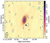 |
Fig. 1. Continuum map, centered at the position of the YSO, combining the eight observations of this work. The color scale indicates the Stokes I emission. Contours identify the Stokes V emission, at a level of −3, −2, 2, 3, 5, and 7 times the Stokes V rms, which is σV ∼ 1.1 μJy beam−1. Negative contours are shown in purple dashes, and positive ones in green-yellow solid lines. The cross (+) marks the position of the tentative brown draft seen in previous VLA observations. The synthesized beam is shown in the lower-left corner. |
There is no conclusive indication of emission from the tentative position of the brown dwarf (marked by a cross in Fig. 1). The expected position has been calculated considering the previous radio observation by Alves et al. (2020) on 2016, October 15th (VLA 16B/260), from which we adopted the coordinates for the tentative sub-stellar object ( ,
,  1) and applied the correction considering the relative shift in the position of YSO compared to the previous VLA detection (Alves et al. 2020). The shift in the position of the YSO is within the proper motion reported for Gaia DR3 (Gaia Collaboration 2016, 2023), source ID 4108624199978985984 (adopted by Zurlo et al. 2021 as well): μα = −3.67 ± 0.60 mas yr−1, μδ = −17.94 ± 0.41 mas yr−1. Also, we can estimate the orbital period of the putative brown dwarf to be ∼2.3 centuries, assuming a Keplerian circular orbit at ∼50 au separation and stellar mass of M ∼ 2.2 M⊙ (Alves et al. 2020). The corresponding orbital motion covered in ∼5.5 years would be ∼2.4% of the orbit (meaning ∼40 mas), comparable with the proper motion of the system. We account for an overall ∼40 mas uncertainty in the position of the sub-stellar object, which is indicated by the size of the cross.
The 2σ contour in Stokes V in Fig. 1 are nearly in agreement with such location. This is suggestive, but statistically not sufficient to claim a detection of the sub-stellar object. Considering the rms for the total integrated map, we set a 3σ upper limit of ∼3.6 μJy to the 15 GHz emission from the putative sub-stellar object.
3.2. Variable flux in Stokes I across the different epochs
As the observations were spread over a month, we also searched for possible variability in the signal from the YSO over different observing days and within each of them. A detailed description is presented in the following sections. We report in Table 2 the detailed analysis for each epoch and for the combined image discussed above. We show the images of Stokes I (in color) and Stokes V (in contours) for each observing run in Fig. 2. The YSO is clearly detected in all of them in Stokes I. A right circular polarized signal is clearly detected on March 5 and March 26, with a marginal detection on March 9, and no detections in the other five observations.
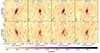 |
Fig. 2. Images for each observation (day indicated in the label) for Stokes I, with Stokes V overlaid in contours. The contour levels are color coded and represent −3, −2, 2, 3, 5, 7, and 8 times the σ, which ranges from 3 to 4 μJy beam−1 (see Table 1). The synthesized beam for each day is shown in the lower left corner, while the cross + marks the position of the potential sub-stellar companion as seen in previous observations. The position has been corrected, taking into consideration the proper motion of the YSO from the Gaia database. |
In correspondence with the position of the sub-stellar object (marked by a cross with the width corresponding to the aforementioned uncertainty), we only see a marginal and insignificant detection during the first observation of March 10 and March 27 in Stokes V (S/N ∼ 2 − 3σ). In Stokes I, it is much more difficult to evaluate excess at few tens μJy level at the same position because of the brighter central emission (we have also tried to use a briggs weighting to enhance the resolution); visually, the only suggestive case is on March 30th with a S/N ∼ 5σ (possibly helped by the lowest flux from the central star on that day). We can neither claim or discard the possibility of an excess at the plausible sub-stellar position.
Figure 3 shows the total flux density in Stokes I, with significant variability across the observational window spanning 27 days. During these eight epochs, the flux values fluctuated, from the highest on the first day, March 5, with an integrated flux of 216 μJy, to the minimum value of ∼108 μJy on March 30. Such variations can rise up to a factor of ∼2 – and much higher than the flux errors. The variable behavior is seen in both peak and integrated fluxes. Overall, the variations did not exhibit any discernible or predictable pattern. As a matter of fact, between the observations of March 26–27, the integrated flux decreased by ∼1/4 in 22 h, pointing to substantial variations in ≲1 day. Similarly, there is a significant flux increase between March 30–31. On the other hand, the three closest observations between March 9th and 10th show integrated fluxes compatible within 2σ to each other. These erratic, variability timescales (on the order of about a day) can be indicative of processes coming from the YSO itself or the immediate surroundings.
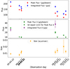 |
Fig. 3. Variability over the over the eight observational epochs. We show the peak flux intensity and the integrated flux density in Stokes I (top) and Stokes V (middle), and the size of the deconvolved component of the emission in Stokes I, calculated by using the values and errors of the major and minor axes in Table 2. Vertical bars show 1σ errors. For the days without a Stokes V detection, we have provided 3σ upper limits for the peak flux. |
The signs for a slightly resolved extended emission, discussed above for the combined images, are consistently seen in each observation as well: the peak flux is systematically ∼20 − 30% lower than the integrated flux and the reconstructed values of the deconvolved Stokes I components are slightly larger than the clean beams (see Table 2). A complementary analysis of the amplitude versus uv-distance profiles did not shed further light in this aspect, because the fluctuations are not small enough to distinguish between a point source and slightly resolved emission.
3.3. Circularly polarized signal in two epochs
To look for a circularly polarized signal, we analyzed the Stokes V images as well. We obtained significant Stokes V detections with ∼9σ and ∼6σ in the March 5 and March 26 observations, with a polarization fraction of about 16 − 18%. For the rest of the days without a detection, we set 3σ upper limits of the order of 10 μJy/beam, corresponding to circular polarization upper limits in the range between ∼5 and 12%. We also combined the remaining six datasets without a Stokes V detection, in order to slightly improve their rms, but only found a non significant S/N ∼ 2σ Stokes V signal.
Table 2 also shows the peak and integrated flux densities of the Stokes V signal (or the 3σ upper limit in the absence of detection) for each epoch. The sporadicity of the emission seen here is typical of circularly polarized radiation driven by plasma emission or electron cyclotron maser (ECM) emission. High polarization fractions are expected for these mechanisms (Dulk 1985), which may be consistent with the moderate values observed here if we consider the superposition with a persistent, unpolarized component. In this sense, it is significant to note that the difference of Stokes I flux between the days (March 5 and 26) with Stokes V detection and the following available observations (March 9 and 27) are positive and of the same order of the detected Stokes V. We do not have enough observational cadence to confirm this suggestion, that would point to a ∼100% polarized component in addition to the persistent one.
Alternatively, incoherent gyro-synchrotron emission from mildly relativistic electrons can also provide modest circular polarization. We also note that, considering a tentative 3σ detection during the March 9 observation and the upper limits in the remaining observations, we cannot discard a persistent but variable weak polarization, which would again favour gyro-synchrotron.
3.4. Frequency dependence of the emission
We investigated the frequency dependence of the emission, by combining all days, using the CASA task specflux. As shown in the lower panel of Fig. 4, the flux-frequency curve looks flat within the uncertainties, with the flux density only slightly increasing with frequencies. Additionally, we inferred the spectral index on a scan-by-scan basis, by looking at the slope between 12–15 GHz and 15–18 GHz flux density. All spectral indexes are close to flat or slightly positive (−0.16 < α < 0.5) and compatible with each other within the (large) errors.
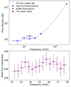 |
Fig. 4. Broadband spectrum of flux density for the YSO in Stokes I (top), considering all available VLA (4–35 GHz) and ALMA (230 GHz) data (Dzib et al. 2016; Alves et al. 2020; Zurlo et al. 2021). The horizontal bars represent the bandwidth for each observed band. Spectral distribution of mean flux in Stokes I for the current VLA observations (bottom) averaged over all days and over three spectral windows, i.e., 384 MHz. The vertical error bars correspond to the 1σ, while the width of the horizontal bars is equivalent to the bandwidth of 384 MHz over which each data point has been averaged. |
To set these results in the context of a broader frequency range, we also show in Fig. 4 the global spectrum where past VLA and ALMA observations are considered, from 4 to 230 GHz (Dzib et al. 2016; Alves et al. 2020). Overall, there is an apparent change of slope seen just around the 15 GHz band studied here. Indeed, this is consistent with the almost flat spectrum seen in our data. The change in slope is probably due to the co-existence of the (gyro-)synchrotron emission (negative slope, dominating at low frequencies) and free-free emission (positive slope, higher frequencies). We also note that the flux detected in the current observations is slightly higher than in the past.
3.5. Short-term variability
We investigated the possible contributions to the flux variability from short flaring events. We examined fluctuations in the peak flux intensity during individual observing sessions.
First, we looked at the dynamic spectra, shown in Fig. 5 for March 26, one of the two days with a clear Stokes V detection. We show the results for Stokes I (top panel) and Stokes V (bottom). It is possible that due to the rms fluctuations, there is no visible spike (in time) or spectral features for both Stokes I and V. The emission seems to increase slightly with frequency, in agreement with the slightly positive spectral index found in that day’s observation when split into two bands, as mentioned before (α = 0.33 ± 0.25).
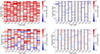 |
Fig. 5. Dynamic spectrum of a region encompassing the source (left) and another region away from the phase center for the March 26th observation, in Stokes I (top) and Stokes V (bottom). The dynamic spectrum has been obtained selecting the source from the image plane and integrating over 256 MHz-wide spectral windows, for each scan (approximately 6 min long). On average, the rms in each pixel is ∼70 μJy beam−1 for each scan in both Stokes I and Stokes V. The thin vertical black lines between target scans represent the time spent on the phase calibrator (∼48 s). The panels on the right side have been plotted only to present a visual comparison between the flux values during the presence and absence of a radio source. To obtain these spectra, we used the CASA task specflux and imstat after generating the cube images with tclean, for every source scan. |
To investigate this on shorter timescales, we divided the data from each session into shorter integration times of 10, 30, and 60 s, by integrating the data over all the channels to have a high enough S/N. For this purpose, we used the CASA task visstat to calculate the statistics separately for the LL and RR correlators and obtained Stokes I ((RR+LL)/2) and Stokes V ((RR-LL)/2) statistics. We did not find any clear, structured spikes in any epoch, although there were a few single-point spikes with S/N > 5, but with no conclusive periodic behavior (see Appendix A for the plots showing the time series for an integration time of 60 s for all the days). To look for periodicity in these data sets, we also obtained the GLS periodogram (Zechmeister & Kürster 2018), which gave us no statistically significant peak (False Alarm Probability < 1%) in the Fourier space at any epoch. In summary, we did not find any sign of short (minutes or sub-minutes) clear variability or spikes.
4. Discussion and conclusions
YSO [BHB2007]-1 is a peculiar object, showing interesting properties across the radio/mm spectrum. Here, we present a detailed analysis of eight observations taken with VLA at 15 GHz. We clearly detected the radio emission from the central YSO, with a slightly resolved emission. The observed radio emission also has a mild variability on timescales of a few days, with no clear minute or sub-minute variability trend.
The spectral index is slightly positive – and not entirely incompatible with being flat in nature. Combined with previous data from VLA and ALMA between 10 and 230 GHz, there does indeed seem to be a spectral turning point right at the Ku band (15 GHz), which is being explored in this study. This is compatible with the presence of two components: a free–free emission component and a non-thermal component. The free–free emission is probably related with collimated winds observed in CO (Alves et al. 2020) and tentatively detected in the near-IR (Zurlo et al. 2021), while the non-thermal component, predominantly (gyro-)synchrotron, has a negative slope and dominates at lower frequencies. Therefore, the detection of a non-thermal component becomes more difficult at higher frequencies where free free emission becomes prominent (Güdel 2002).
In agreement with this interpretation, we found two epochs with a clear Stokes V detection of ∼16 − 18%. The lack of such detection in other epochs is compatible with the presence of a sporadic, possibly moderate or highly circularly polarized non-thermal component, coming on top of the persistent, thermal one. Among non-thermal processes, gyro-synchrotron emission can provide moderate values of circular polarization (Dulk 1985; Andre 1996), while the coherent plasma emission or ECM would tend to exhibit larger polarization fractions (Dulk 1985; Treumann 2006; Bastian et al. 2022; Berger et al. 2008; Yiu et al. 2024; Callingham et al. 2021).
The Stokes V emission seems to be slightly resolved as well. In this scenario, the non-thermal component would originate from electrons in the surroundings, which gyrate around the magnetic fields. The resulting polarization fraction strongly depends on the electron energy and may be characterized by moderate values for mildly relativistic electrons, with Lorentz factors of γ ≤ 2 − 3 (Dulk 1985). In this context, the jet-induced shocks could also be accelerating the electrons to such mildly relativistic energies, thereby contributing to the observed non-thermal emission (Feigelson & Montmerle 1999; Miettinen et al. 2008; Ainsworth et al. 2014). It is worth noting that in the epochs where we have clearly detected circularly polarized emission, the integrated flux density for Stokes I emission appears to have increased by a similar amount (within the errors) of the Stokes V, with respect to the observations made just after the stokes V detection (see Table 2). Since the observed level of circular polarization depends also on the contemporaneous presence of the unpolarized components, in this regard, we cannot discard the possible sporadic presence of an additional highly circularly polarized component that is possibly disconnected from the main one and driven by coherent mechanisms akin to ECM or plasma emission. If driven by the ECM, the radio emission holds direct information about the magnetic fields at play, with ν = 2.8 B[G] MHz (ν is the cut-off frequency). This suggests the local magnetic field to be < 6.4 kG, assuming a cut-off frequency ∼18 GHz (upper limit of Ku band).
The slightly resolved emission also hints at the possibility that the emission is composed by more than one component: one of them contributing to the thermal emission and the other one responsible for the (partially sporadic) non-thermal component. This may be compatible with both a single or a binary star. The possibility of a radio binary (unresolved so far) would be supported by the fact that the dynamical mass of the source is twice the mass expected from near-IR observations (Zurlo et al. 2021; Alves et al. 2020). Since the emission patterns from [BHB2007]-1 have been previously seen in other radio binaries (Girart et al. 2000, 2004), this scenario deserves further investigation. A very well known example, with some analogies to our case, is the southern radio source (T Tau Sr) in the T Tauri multiple star system (Loinard et al. 2007). One of this components produces time-variable, circularly polarized radio emission as also observed for two epochs of [BHB2007]-1, while the other component is extended, unpolarized and only moderately variable, with a spectral index typical of optically thin free-free radiation. Past studies have proposed that this variable, polarized emission may have a magnetic origin (Phillips et al. 1993; Smith et al. 2003); whereas the free-free component may have been produced by the interaction of a supersonic stellar wind driven by T Tau Sb and dense surrounding material that is possibly associated with the circumbinary structure around the pair (Loinard et al. 2007).
Finally, we could not clearly detect the sub-stellar object that is said to be opening up a visible gap in the disk (Alves et al. 2020; Zurlo et al. 2021), although we do see marginal Stokes V signals in two of the epochs, as explained in Sect. 3. Apart from that, there also appears a weak Stokes I signal around the proposed position of the sub-stellar object in one of the observations taken on March 30, 2022, but the emission does not coincide exactly with the position of the sub-stellar object.
In this respect, we suggest that it would be ideal to cover both the low-frequency (GHz and below) and the 50–200 GHz window in the future to monitor the variability and the overall spectrum of this YSO. In particular, additional data in Stokes V might shed some light on the nature of the polarized component. Finally, it would be very important to search for signatures of the tentative radio companion.
Acknowledgments
SK, JMG, DV, ASM, OM and FDS’s work is partially supported by the program Unidad de Excelencia María de Maeztu, awarded to the Institut de Ciències de l’Espai (CEX2020-001058-M). SK carried out this work within the framework of the doctoral program in Physics of the Universitat autònoma de Barcelona. SK, DV and OM are supported by the European Research Council (ERC) under the European Union’s Horizon 2020 research and innovation programme (ERC Starting Grant “IMAGINE” No. 948582, PI: DV). JMG acknowleges support by grant PID2020-117710GB-I00(MCI-AEI-FEDER,UE). AZ acknowledges support from ANID – Millennium Science Initiative Program – Center Code NCN2021_080. FDS acknowledges support from a Marie Curie Action of the European Union (Grant agreement 101030103). T.B. acknowledges financial support from the FONDECYT postdoctorado project number 3230470. This work has also made use of data from the European Space Agency (ESA) mission Gaia (https://www.cosmos.esa.int/gaia), processed by the Gaia Data Processing and Analysis Consortium (DPAC, https://www.cosmos.esa.int/web/gaia/dpac/consortium) Funding for the DPAC has been provided by national institutions, in particular the institutions participating in the Gaia Multilateral Agreement.
References
- Ainsworth, R. E., Scaife, A. M. M., Ray, T. P., et al. 2014, ApJ, 792, L18 [Google Scholar]
- Alves, F. O., Cleeves, L. I., Girart, J. M., et al. 2020, ApJ, 904, L6 [NASA ADS] [CrossRef] [Google Scholar]
- Andre, P. 1996, ASP Conf. Ser., 93, 273 [NASA ADS] [Google Scholar]
- Anglada, G. 2017, in Highlights on Spanish Astrophysics IX, eds. S. Arribas, A. Alonso-Herrero, F. Figueras, C. Hernández-Monteagudo, A. Sánchez-Lavega, & S. Pérez-Hoyos, 1 [Google Scholar]
- Anglada, G., Rodríguez, L. F., & Carrasco-González, C. 2018, A&ARv, 26, 3 [Google Scholar]
- Bastian, T. S., Cotton, W. D., & Hallinan, G. 2022, ApJ, 935, 99 [NASA ADS] [CrossRef] [Google Scholar]
- Berger, E., Gizis, J. E., Giampapa, M. S., et al. 2008, ApJ, 673, 1080 [NASA ADS] [CrossRef] [Google Scholar]
- Callingham, J. R., Vedantham, H. K., Shimwell, T. W., et al. 2021, Nat. Astron., 5, 1233 [NASA ADS] [CrossRef] [Google Scholar]
- CASA Team (Bean, B., et al.) 2022, PASP, 134, 114501 [NASA ADS] [CrossRef] [Google Scholar]
- Comrie, A., Wang, K. S., Hsu, S. C., et al. 2021, Astrophysics Source Code Library [record ascl:2103.031] [Google Scholar]
- Covey, K. R., Lada, C. J., Román-Zúñiga, C., et al. 2010, ApJ, 722, 971 [NASA ADS] [CrossRef] [Google Scholar]
- Díaz-Márquez, E., Grau, R., Busquet, G., et al. 2024, A&A, 682, A180 [NASA ADS] [CrossRef] [EDP Sciences] [Google Scholar]
- Dulk, G. A. 1985, ARA&A, 23, 169 [Google Scholar]
- Dzib, S. A., Loinard, L., Medina, S. N. X., et al. 2016, Rev. Mex. Astron. Astrofis., 52, 317 [Google Scholar]
- Dzib, S. A., Loinard, L., Ortiz-León, G. N., Rodríguez, L. F., & Galli, P. A. B. 2018, ApJ, 867, 151 [Google Scholar]
- Farrell, W. M., Desch, M. D., & Zarka, P. 1999, J. Geophys. Res., 104, 14025 [NASA ADS] [CrossRef] [Google Scholar]
- Feeney-Johansson, A., Purser, S. J. D., Ray, T. P., et al. 2019, ApJ, 885, L7 [Google Scholar]
- Feigelson, E. D., & Montmerle, T. 1999, ARA&A, 37, 363 [Google Scholar]
- Forbrich, J., Preibisch, T., & Menten, K. M. 2006, A&A, 446, 155 [NASA ADS] [CrossRef] [EDP Sciences] [Google Scholar]
- Gaia Collaboration (Prusti, T., et al.) 2016, A&A, 595, A1 [NASA ADS] [CrossRef] [EDP Sciences] [Google Scholar]
- Gaia Collaboration (Vallenari, A., et al.) 2023, A&A, 674, A1 [NASA ADS] [CrossRef] [EDP Sciences] [Google Scholar]
- Girart, J. M., Rodríguez, L. F., & Curiel, S. 2000, ApJ, 544, L153 [NASA ADS] [CrossRef] [Google Scholar]
- Girart, J. M., Curiel, S., Rodríguez, L. F., et al. 2004, AJ, 127, 2969 [NASA ADS] [CrossRef] [Google Scholar]
- Güdel, M. 2002, ARA&A, 40, 217 [Google Scholar]
- Loinard, L., Rodríguez, L. F., D’Alessio, P., Rodríguez, M. I., & González, R. F. 2007, ApJ, 657, 916 [NASA ADS] [CrossRef] [Google Scholar]
- Lovell, J. B., Keating, G. K., Wilner, D. J., et al. 2024, ApJ, 962, L12 [NASA ADS] [CrossRef] [Google Scholar]
- Meng, F., Sánchez-Monge, Á., Schilke, P., et al. 2019, A&A, 630, A73 [NASA ADS] [CrossRef] [EDP Sciences] [Google Scholar]
- Miettinen, O., Kontinen, S., Harju, J., & Higdon, J. L. 2008, A&A, 486, 799 [NASA ADS] [CrossRef] [EDP Sciences] [Google Scholar]
- Obonyo, W. O., Lumsden, S. L., Hoare, M. G., et al. 2019, MNRAS, 486, 3664 [Google Scholar]
- Ott, J., Raba, R., & Hibbard, J. 2022, Am. Astron. Soc. Meet. Abstr., 54, 215.05 [Google Scholar]
- Pech, G., Loinard, L., Dzib, S. A., et al. 2016, ApJ, 818, 116 [Google Scholar]
- Phillips, R. B., Lonsdale, C. J., & Feigelson, E. D. 1993, ApJ, 403, L43 [NASA ADS] [CrossRef] [Google Scholar]
- Pineda, J. S., & Villadsen, J. 2023, Nat. Astron., 7, 569 [NASA ADS] [CrossRef] [Google Scholar]
- Scaife, A. 2012, Astron. Rev., 7, 26 [Google Scholar]
- Shang, H., Lizano, S., Glassgold, A., & Shu, F. 2004, ApJ, 612, L69 [NASA ADS] [CrossRef] [Google Scholar]
- Smith, K., Pestalozzi, M., Güdel, M., Conway, J., & Benz, A. O. 2003, A&A, 406, 957 [NASA ADS] [CrossRef] [EDP Sciences] [Google Scholar]
- Stevens, I. R. 2005, MNRAS, 356, 1053 [NASA ADS] [CrossRef] [Google Scholar]
- Treumann, R. A. 2006, A&ARv, 13, 229 [Google Scholar]
- Vargas-González, J., Forbrich, J., Rivilla, V. M., et al. 2023, MNRAS, 522, 56 [CrossRef] [Google Scholar]
- Yiu, T. W. H., Vedantham, H. K., Callingham, J. R., & Günther, M. N. 2024, A&A, 684, A3 [NASA ADS] [CrossRef] [EDP Sciences] [Google Scholar]
- Zarka, P. 2007, Planet. Space Sci., 55, 598 [Google Scholar]
- Zechmeister, M., & Kürster, M. 2018, Astrophysics Source Code Library [record ascl:1807.019] [Google Scholar]
- Zurlo, A., Garufi, A., Pérez, S., et al. 2021, ApJ, 912, 64 [NASA ADS] [CrossRef] [Google Scholar]
Appendix A: Time series for all the observations
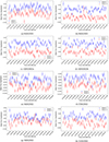 |
Fig. A.1. 60-second time series for all the epochs in Stokes I and Stokes V. These plots have been generated by plotting the real part of the amplitude versus time for the target field, using CASA task visstat. The error bars represent the statistically calculated standard deviation in the data. |
All Tables
Statistics of fluxes and deconvolved emission, from Gaussian fitting of the clean images of each day.
All Figures
|
Fig. 1. Continuum map, centered at the position of the YSO, combining the eight observations of this work. The color scale indicates the Stokes I emission. Contours identify the Stokes V emission, at a level of −3, −2, 2, 3, 5, and 7 times the Stokes V rms, which is σV ∼ 1.1 μJy beam−1. Negative contours are shown in purple dashes, and positive ones in green-yellow solid lines. The cross (+) marks the position of the tentative brown draft seen in previous VLA observations. The synthesized beam is shown in the lower-left corner. |
| In the text | |
|
Fig. 2. Images for each observation (day indicated in the label) for Stokes I, with Stokes V overlaid in contours. The contour levels are color coded and represent −3, −2, 2, 3, 5, 7, and 8 times the σ, which ranges from 3 to 4 μJy beam−1 (see Table 1). The synthesized beam for each day is shown in the lower left corner, while the cross + marks the position of the potential sub-stellar companion as seen in previous observations. The position has been corrected, taking into consideration the proper motion of the YSO from the Gaia database. |
| In the text | |
|
Fig. 3. Variability over the over the eight observational epochs. We show the peak flux intensity and the integrated flux density in Stokes I (top) and Stokes V (middle), and the size of the deconvolved component of the emission in Stokes I, calculated by using the values and errors of the major and minor axes in Table 2. Vertical bars show 1σ errors. For the days without a Stokes V detection, we have provided 3σ upper limits for the peak flux. |
| In the text | |
|
Fig. 4. Broadband spectrum of flux density for the YSO in Stokes I (top), considering all available VLA (4–35 GHz) and ALMA (230 GHz) data (Dzib et al. 2016; Alves et al. 2020; Zurlo et al. 2021). The horizontal bars represent the bandwidth for each observed band. Spectral distribution of mean flux in Stokes I for the current VLA observations (bottom) averaged over all days and over three spectral windows, i.e., 384 MHz. The vertical error bars correspond to the 1σ, while the width of the horizontal bars is equivalent to the bandwidth of 384 MHz over which each data point has been averaged. |
| In the text | |
|
Fig. 5. Dynamic spectrum of a region encompassing the source (left) and another region away from the phase center for the March 26th observation, in Stokes I (top) and Stokes V (bottom). The dynamic spectrum has been obtained selecting the source from the image plane and integrating over 256 MHz-wide spectral windows, for each scan (approximately 6 min long). On average, the rms in each pixel is ∼70 μJy beam−1 for each scan in both Stokes I and Stokes V. The thin vertical black lines between target scans represent the time spent on the phase calibrator (∼48 s). The panels on the right side have been plotted only to present a visual comparison between the flux values during the presence and absence of a radio source. To obtain these spectra, we used the CASA task specflux and imstat after generating the cube images with tclean, for every source scan. |
| In the text | |
|
Fig. A.1. 60-second time series for all the epochs in Stokes I and Stokes V. These plots have been generated by plotting the real part of the amplitude versus time for the target field, using CASA task visstat. The error bars represent the statistically calculated standard deviation in the data. |
| In the text | |
Current usage metrics show cumulative count of Article Views (full-text article views including HTML views, PDF and ePub downloads, according to the available data) and Abstracts Views on Vision4Press platform.
Data correspond to usage on the plateform after 2015. The current usage metrics is available 48-96 hours after online publication and is updated daily on week days.
Initial download of the metrics may take a while.