| Issue |
A&A
Volume 690, October 2024
|
|
|---|---|---|
| Article Number | A294 | |
| Number of page(s) | 20 | |
| Section | Interstellar and circumstellar matter | |
| DOI | https://doi.org/10.1051/0004-6361/202450530 | |
| Published online | 17 October 2024 | |
The [O I] fine structure line profiles in Mon R2 and M17 SW: The puzzling nature of cold foreground material identified by [12C II] self-absorption
1
I. Physikalisches Institut, Universität zu Köln,
Zülpicher Str. 77,
50937
Köln,
Germany
2
Instituto de Astronomía, Universidad Católica del Norte,
Av. Angamos 0610,
1270398
Antofagasta,
Chile
3
Jet Propulsion Laboratory, California Institute of Technology,
4800 Oak Grove Drive,
Pasadena,
CA
91109-8099,
USA
4
European Southern Observatory,
Alonso de Córdova 3107,
Vitacura, Santiago,
Chile
5
Institute of Optical Sensor Systems, German Aerospace Center (DLR),
Rutherfordstr. 2,
12489
Berlin,
Germany
6
Max-Planck-Institut für Radioastronomie,
Auf dem Hügel 69,
53121
Bonn,
Germany
7
Centro de Astro-Ingeniería UC, Instituto de Astrofísica, Pontificia Universidad Católica de Chile,
Avda Vicuña Mackenna 4860,
Macul, Santiago,
Chile
★ Corresponding author; This email address is being protected from spambots. You need JavaScript enabled to view it.
Received:
26
April
2024
Accepted:
16
September
2024
Abstract
Context. Recent studies of the optical depth comparing [12C II] and [13C II] line profiles in Galactic star-forming regions have revealed strong self-absorption in [12C II] by low excitation foreground material. This implies a high column density for C+, corresponding to equivalent AV values of a few (up to about 10) mag.
Aims. As the nature and origin of such a great column of cold C+ foreground gas are difficult to determine, it is essential to constrain the physical conditions of this material.
Methods. We conducted high-resolution observations of [O I] 63 μm and [O I] 145 μm lines in M17 SW and Mon R2. The [O I] 145 μm transition traces warm PDR-material, while the [O I] 63 μm line traces the foreground material, as manifested by the absorption dips.
Results. A comparison of both [O I] line profiles with [C II] isotopic lines confirm warm PDR-origin background emission and a significant column of cold foreground material, causing the self-absorption to be visible in the [12C II] and [O I] 63 μm profiles. In M17 SW, the C+ and O0 column densities are comparable for both layers. Mon R2 exhibits larger O0 columns compared to C+, indicating additional material where the carbon is neutral or in molecular form. Small-scale spatial variations in the foreground absorption profiles and the large column density (~1018 cm−2) of the foreground material suggest the emission is coming from high-density regions associated with the cloud complex – and not a uniform diffuse foreground cloud.
Conclusions. The analysis confirms that the previously detected intense [C II] foreground absorption is attributable to a large column of low-excitation dense atomic material, where carbon is ionized and oxygen is in a neutral atomic form.
Key words: ISM: atoms / ISM: clouds / ISM: general / ISM: lines and bands / photon-dominated region (PDR) / ISM: structure
© The Authors 2024
 Open Access article, published by EDP Sciences, under the terms of the Creative Commons Attribution License (https://creativecommons.org/licenses/by/4.0), which permits unrestricted use, distribution, and reproduction in any medium, provided the original work is properly cited.
This article is published in open access under the Subscribe to Open model. This email address is being protected from spambots. You need JavaScript enabled to view it. to support open access publication.
1 Introduction
The fine structure emission lines of [O I], together with the [C II] 158 μm emission line and high-J CO lines, are the main cooling lines for photodissociation regions (PDRs, Tielens & Hollenbach 1985; Hollenbach & Tielens 1999) in the interstellar medium (ISM). The spin-orbit coupling in neutral atomic oxygen leads to three fine-structure levels and, correspondingly, two [O I] fine structure transitions. The lower transition, [O I] 3P1 → 3P2, has a wavelength of 63.2 μm, corresponding to an energy of its upper level of 227.7 K; the collisional rate coefficients with H give a critical density at 77 K of 7.8×105 cm−3, and with H2 as collision partner, the critical density is 5×105 cm−3 (Goldsmith 2019). The upper transition, [O I] 3P0 →3P1, has a wavelength of 145.5 μm. Its upper state energy is 326.6 K above the ground state, or 98.9 K above the mid-level, with a critical density of 5.8×106 cm−3 for H2 as collision partner (Goldsmith 2019). The [O I] fine structure emission from PDRs is thus bright if the gas is dense. It is, therefore, together with the [C II] 158 μm fine structure line, commonly used for tracing the warm and dense gas in star-forming regions, locally and out to high red-shift galaxies. The [O I] 63 μm transition rapidly reaches a high optical depth in low-temperature gas (T≪ 230 K), so high that the intensity is no longer a measure of the column density. The fine structure lines of the oxygen isotopes (in particular 18O) are so close in frequency that they blend with the Doppler-broadened main isotope transition in astronomical sources so that the iso-topic line ratios cannot be used to determine the [O I] optical depth. Early indications of high optical depth have been reported by Stacey et al. (1983) and Boreiko & Betz (1996) based on a comparison of the integrated line intensity ratio of the [O I] lines, but the optical depth could be only inferred indirectly. High signal-to-noise (S/N) line profiles are required to directly measure the fine structure line optical depth, showing saturation or self-absorption. With the high spectral resolution and high S/N available with the GREAT (Heyminck et al. 2012) instrument on the Stratospheric Observatory for Infrared Astronomy (SOFIA, Young et al. 2012; Temi et al. 2018), several authors Leurini et al. (2015); Schneider et al. (2018); Mookerjea et al. (2019); Kirsanova et al. (2020); Goldsmith et al. (2021) have recently reported velocity resolved [O I] 63 μm observations displaying complex line profiles. A recent survey of [O I] 63 μm line profiles towards 12 star-forming cores in the Milky Way by Goldsmith et al. (2021) showed self-absorption by foreground material for half of the sources. In addition, high optical depth and self-absorption in [O I] are often invoked to explain the observed too-low [O I] 63 μm intensities compared to model predictions from other observed lines.
In a recent study of several Galactic star-forming regions comparing the [12 Cii] and [13C II] line profiles at high S/N (Guevara et al. 2020), we have shown that the [C II] 158 μm emission is optically thick in a wide range of physical conditions. The two sources, Monoceros R2 (Mon R2) and M17 SW, were studied and showed deep and narrow self-absorption in the line profiles against the bright and broad background line emission. The analysis of those spectra showed that the bright background line emission, derived from the optically thin [13C II] line profile and compatible with originating in PDRs, is absorbed by a large column density of ionized carbon in cold foreground material, with a low excitation temperature (Tex ≲ 25 K). A lower limit for the foreground material, derived under the assumption that all carbon is in the form of C+, gives a corresponding visual extinction of several (up to ten) magnitudes. The amount of material can be considerably larger if the carbon is only partially ionized and the foreground gas contains more carbon in the form of neutral atoms or bound in molecules, particularly CO. However, the velocities and line widths of these foreground absorption features do not match with any features in the spectral lines of carbon monoxide, indicating that the foreground absorbing material presents a component of the ISM that is separate from the molecular gas traced by CO. To present knowledge, ionized carbon is present mainly in PDR layers at temperatures above 60. Hence, the nature of such large amounts of ionized carbon in low excitation layers of gas is very puzzling. Low excitation may imply low density (well below the critical density of [C II]), but such diffuse gas would need to fill large volumes to explain the observed total column density. Kabanovic et al. (2022) presented a scenario for the source RCW 120, where the carbon is present in a diffuse envelope with neutral hydrogen.
Mon R2 is a star-forming region at a distance of 778 pc (Zucker et al. 2019). The region contains a reflection nebula, and the UCH II region is surrounded by several PDRs with different physical conditions. The molecular cloud associated with Mon R2 has a hub-filament structure and contains clumps of density up to 106 cm−3. The radiation field in the interface region between the H II region and the cloud is about 105 Go (Pilleri et al. 2012). The sources have been studied through several atomic and molecular tracers (e.g., Pilleri et al. 2012, 2013; Treviño-Morales et al. 2014; Rayner et al. 2017; Treviño-Morales et al. 2019).
M17 is one of the brightest and most massive star-forming regions in the Galaxy, located at a distance of 1.9 kpc (Wu et al. 2019). M17 SW is the sub-region located in the southwest, where an H II region is localized and is associated with a giant molecular cloud and PDR interface. M17 SW is considered a prototype of an edge-on PDR. The H II region is ionized by a highly obscured (with a visual extinction AV > 10 mag) cluster of many (>100) OB stars (Hoffmeister et al. 2008). The gas near the H II region is distributed in high density clumps (n ≤ 105 cm−3) embedded in interclump material (n ~ 103 cm−3) surrounded by diffuse gas (n ~ 300 cm−3), irradiated by a strong UV field of Go = 5.6×10⁴ (Meixner et al. 1992). Recently, using non-velocity resolved observations of several infrared lines such as [C II], both [O I] lines, [O III], or [N III] from FIFI-LS (Colditz et al. 2018; Fischer et al. 2018), Klein et al. (2023) derived hydrogen nuclei density and UV radiation maps, with an average hydrogen density of 105.9 cm−3 for the molecular cloud. They found that the ionization and photodissociation fronts are nearly merged with a sharp density jump from the ionized region to the neutral one.
To characterize the nature of the absorbing layer in these two sources, Mon R2 and M17 SW, we followed up on the investigation we started in Guevara et al. (2020) by observing the two sources in both [O I] fine structure lines with the upGREAT1 instrument (Risacher et al. 2016) on board SOFIA along the same lines of sight, as previously observed in [C II].
The paper is organized as follows. Section 2 details the observational setup and data reduction. Section 3 shows the observed [O I] 145 μm and [O I] 63 μm line profiles and a comparison against [12C II] and [13C II] profiles. Section 4 presents a multi-component double-layered Gaussian profile analysis using both [O I] lines to estimate oxygen column densities and excitation temperature. Section 5 discusses the results and the possible nature of the background and foreground layers. Finally, Sec. 6 summarizes the present work.
2 Observations and data reduction
We observed the [O I] 63 μm and [O I] 145 μm fine-structure lines in Mon R2 and M17 SW with the 7-pixel High-Frequency Array (HFA) and the 7x2-pixel Low-Frequency Array (LFA) arrays of the upGREAT receiver on board SOFIA. Mon R2 was observed in December 2018, and M17 SW in June 2019 and April 2022. For Mon R2, the LFA was tuned to observe the [O I] 145 μm in the H-polarization array (LFAH) and [C II] 158 μm line in the V-polarization (LFAV) simultaneously. The single-sideband (SSB) system temperatures at the source velocity (Tsys) were 3500 and 3050 K, respectively. In parallel, the HFA was tuned to [O I] 63 μm, with a Tsys(SSB) of 4700 K. The parameters are summarized in Table 1. As the former [C II] spectra (Guevara et al. 2020) were observed with the old singlepixel configuration of the GREAT instrument at two discrete positions, we had no information on the spatial variation of the [C II] line profiles. Hence, we first observed a small, fully sampled map (for the three lines) of 180″×180″ extent in on-the-fly mode with a grid separation of 3″ in the horizontal and vertical directions. Then, we performed deep integrations in total power mode of 5 min ON-source time for the two positions previously observed in [C II] (Fig. 1). Appendix A lists the coordinates of each position in detail and the OFF positions used. The two [C II] positions were selected to follow the peak emission. The average precipitable water vapor column was 7 μm. The OFF position presented some weak contamination of ~2 K, corrected through the same procedure for [C II] as described by Guevara et al. (2020), Appendix B, fitting a Gaussian profile to the OFF position spectra and then adding the fitted profile into the ON spectra to recover the lost emission.
In June 2019, we observed a fully sampled small [O I] map for M17 SW using upGREAT in OTF mode with a grid separation of 3″ in horizontal and vertical directions. The LFA was tuned to simultaneously observe the [O I] 145 μm in LFAH and [C II] 158 μm in LFAV, with a Tsys(SSB) at the velocity of the source of 3000 and 2000 K, respectively. The map has an extent of 220″×220″. The average precipitable water vapor was 8 μm. The HFA was tuned to [O I] 63 μm, but the telluric line was located in the central velocities of the emission profile, rendering the observations useless. Hence, we repeated the same observations in April 2022 at a different time to avoid the telluric line contamination for the [O I] 63 μm emission. The observations were successful, but this time [O I] 145 μm was the line affected by the telluric feature in the central velocities. The average precipitable water vapor was 6.5 μm with a Tsys(SSB) at 63 μm of 5100 K. The [C II] integrated intensity map shown in Fig. 2 is the combination of the observations referred above and a map observed within the SOFIA Feedback Legacy Project2 (Schneider et al. 2020). We note that the full [C II] map will be discussed in a separate publication3. The positions for the analysis below were selected following the [C II] peak emission along the ridge. The seven positions were previously observed in [12C II] and [13C II], already analyzed in Guevara et al. (2020). The OFF position was apparently free of emission.
The data were calibrated to an intensity scale in main beam brightness temperature, Tmb, with the kalibrate task (Guan et al. 2012), part of the standard GREAT pipeline. Then, we subtracted baselines with the CLASS 90 package, part of the GILDAS4 software, and resampled the data to 0.3 km s−1 channel width, the same as used for the [C II] data.
For Mon R2, the atmospheric 63 μm atomic oxygen line at the time of the observation was located at −10 km s−1 LSR-velocity, sufficiently far away from the emission of the source; hence, it did not affect the analysis of the line profile. For an inter-comparison, we have convolved the three maps to a 15 ″ beam size from the nominal 6.3″ for the [O I] 63 μm and 14.1″ for the [O I] 145 μm and [C II] lines. For M17 SW, the maps observed at different times of the year allowed us to avoid the telluric line. Hence, both [O I] maps were convolved to a 15″ beam size on a 5″ grid with a velocity resolution of 0.3 km s−1. All the maps were gridded and convolved into a joint resolution to compare them in identical conditions, avoiding the difference in intensities given by the dissimilar beam sizes.
Observational parameters.
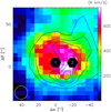 |
Fig. 1 Mon R2 [C II] integrated intensity map for the velocity range between 0 and 30 km s−1 with the two [C II] single pointings (in black) from Guevara et al. (2020). [O I] 63 μm integrated intensity map in blue contours covering the same velocity range of [C II] (levels at 100, 150, 200, 240, 270, and 300 K km s−1). The white circle represents the FWHM beam size of both maps, 15″. |
3 [O I] line profiles
The [C II] and [O I] emission in Mon R2 is compact (see Fig. 1), extending over ≈60″ in all three lines, in contrast to M17 SW, where the emission in both lines is extended along the PDR edge (see Fig. 2). Figure 3 compares the line profiles of the newly observed [O I] spectra in Mon R2 obtained in deep integration and the previously observed [12C II] and [13C II] spectra, the [13C II] profiles shown are the average of the two outer hfs-satellites, as explained in Guevara et al. (2020). The [O I] 145 μm profiles are very similar to those of the [13C II] line, though the latter, being very weak, have a lower S/N. The line profiles agree in peak position and width but also show similarities in the detailed profile structure, which is composed of two Gaussian components overlapping in velocity and added together, as expected for optically thin emission. In contrast, the [O I] 63 μm profile shows deep absorption notches at 8 and 12 km s−1 velocity and possibly a number of additional weaker ones. The overlay with the [12C II] profiles shows that the [O I] absorption matches in center velocity and line width with the self-absorption notches visible in the [12C II] line.
The match in the absorption notches between [12C II] and [O I] 63 μm is present not only in the two positions mentioned above. As shown in Fig. 4, the self-absorption notches are strong across the source and show spatial variation over distances as close as 10″−20″, corresponding to 0.6–0.12 pc at the distance of Mon R2, with changes in intensity at this distances (see Sect. 5.3 for a discussion of this variation).
The absorption to negative intensities (after baseline subtraction) at 11 km s−1 can be explained by a weak 63 μm dust continuum. Additional diffuse gas is present in the line of sight. Pilleri et al. (2013) found foreground absorption through observations of small hydrocarbons at the referenced velocity, with an equivalent AV of 1 magnitude, detached from the source. The absorption by this component is insufficient to explain the absorption dips. However, it may weakly contribute to the absorption at this velocity (see Sec. 3 for an analysis of the absorption dips). The self-absorption notches strongly reduce the [O I] 63 μm integrated intensity. The [O I] 63 μm emission is almost completely absorbed out between 10 and 12 km s−1.
The comparison of the line profiles shows a similar behavior for M17 SW (Fig. 5): the [O I] 145 μm line profile is very similar to the formerly observed [13C II] profiles (where, in this case, the similarity can be confirmed in detail, because of the high S/N of the deep [13C II] integrations). The [O I] 63 μm profiles are heavily affected by self-absorption, and the absorption features are well correlated in position and width with those identified in [12C II] (see the next section for more details). Only the lower velocity component at around 11 km s−1 in the [12C II] line is not reproduced in [O I] 63 μm. As discussed in Guevara et al. (2020), this component is associated with the [N II] emission and also visible in H I, thus presumably associated with diffuse and ionized gas. It is also not traced by the low-J CO lines (Pérez-Beaupuits et al. 2015a,b).
To check for positional variations of the [O I] self-absorption profiles at small angular scales, we plotted a mosaic of the observed line profiles on a grid with 10″ separation, smoothed to the common spatial resolution of 15″. Figure 6 shows the spectra in [O I] 63 μm, [O I] 145 μm and [C II]. The [C II] spectra show spatial variations in their profiles from position to position, namely across 10″, respectively, 0.10 pc, both in the absorption depth and the velocity of the absorption dips. The variations are similarly present in the [O I] 63 μm spectra, although the deep absorption down to close to the zero intensity level makes the variations less pronounced in intensity. The velocities of the absorption dips are well correlated between the [O I] 63 μm and the [C II] emission (same as above, see Sec. 5.3). In contrast, the [O I] 145 μm shows a relatively simple profile of smoothly superimposed emission components.
Table 2 compares the peak and integrated intensities between both [O I] line transitions for both sources. In general, the [O I] 145 μm peak intensity overshoots the [O I] 63 μm peak intensity by a factor of a few due to the self-absorption effect, except for M17 SW position 4. The latter shows a comparable peak intensity but at different velocities, again a result of self-absorption. The difference is more evident in the integrated intensity, with relatively greater [O I] 145 μm integrated intensities, giving a 145/63 integrated intensity ratio between 1.2 and 7. The self-absorption effects thus significantly enhance the integrated intensity ratio. This effect must be considered when analyzing data, particularly non-resolved data without velocity information, such as high-redshift extragalactic observations. Although this self-absorption effect has already been observed under different environments of Galactic molecular clouds (such as Leurini et al. 2015; Gusdorf et al. 2017; Kristensen et al. 2017; Schneider et al. 2018, and references there in), it has also been observed in the large scale [O I] 63 μm spectra of extragalactic sources such as Arp 220, NGC 4945, NGC 4418, and even in the [O III] 88 μm of IRAS17208- 0014 (e.g. González-Alfonso et al. 2012; Fernández-Ontiveros et al. 2016).
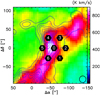 |
Fig. 2 M17 SW [C II] integrated intensity map for the velocity range between 0 and 40 km s−1 with the original [C II] single pointings (in black) from Guevara et al. (2020) (equivalent to a LFA array pointing). [O I] 63 μm integrated intensity map in blue contours covering the same velocity range of [C II] (levels at 40, 70, 100, 120, 140, and 160 and 200 K km s−1). The black circle shows the FWHM beam size for both maps, 15″. |
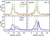 |
Fig. 3 Mon R2 [O I] 63 μm, [O I] 145 μm, [12C II] and [13C II] spectra for the single pointings previously observed in [C II]. All spectra have been convolved to a beam size of 15″. The vertical dashed lines at the 8 and 11 km s−1 absorption dip are present in both spectra, below the horizontal dashed line at 0 K. The [13C II] has been smoothed in velocity for a matter of display. |
4 Gaussian multi-component analysis
For a quantitative comparison, we utilized a two-layer radiative transfer model (Gaussian multi-component fit to the [O I] profiles) that is similar to what we introduced in our previous [12C II] and [13C II] study (Guevara et al. 2020). The formal solution of the radiative transfer equation for a two-layer model with b = 1... B number of background components and f = 1...F number of foreground components gives for the brightness temperature of the line transition t (t = 145, 63 denoting the [O I] 145 μm and the [O I] 63 μm transition respectively):
![Mathematical equation: $\[\begin{aligned}T_{\mathrm{mb}, t}(v)= & {\left[\mathcal{J}_v\left(T_{\mathrm{ex}_t}\right)\left(1-\exp \left(-\sum_b \tau_{b, t}(v)\right)\right)\right] \exp \left(-\sum_f \tau_{f, t}(v)\right) } \\& +\mathcal{J}_v\left(T_{\mathrm{ex}_t}\right)\left(1-\exp \left(-\sum_f \tau_{f, t}(v)\right)\right).\end{aligned}\]$](/articles/aa/full_html/2024/10/aa50530-24/aa50530-24-eq1.png) (1)
(1)
Here, ![Mathematical equation: $\[\mathcal{J}_\nu(T)=\frac{h \nu}{k}\left(e^{h \nu / k_{\mathrm{b}} T}-1\right)^{-1}\]$](/articles/aa/full_html/2024/10/aa50530-24/aa50530-24-eq4.png) is the expression for the equivalent brightness temperature of a blackbody emission at temperature, T. The optical depth of each transition, t, and component i = b, f is given by:
is the expression for the equivalent brightness temperature of a blackbody emission at temperature, T. The optical depth of each transition, t, and component i = b, f is given by:
![Mathematical equation: $\[\tau_{i, t}(v)=\frac{c^3}{8 \pi \nu_t^3} \phi_i(v) N_{u_t, i} A_t\left(\exp \left(h \nu_t /\left(k_b T_{\mathrm{ex}_{i,t}}\right)\right)-1\right),\]$](/articles/aa/full_html/2024/10/aa50530-24/aa50530-24-eq5.png) (2)
(2)
with the upper and lower state of transition t given by ut and 1t respectively, its upper state column density by ![Mathematical equation: $\[N_{\mathrm{u}_t, i}\]$](/articles/aa/full_html/2024/10/aa50530-24/aa50530-24-eq6.png) , and its Einstein-A-coefficients,
, and its Einstein-A-coefficients, ![Mathematical equation: $\[A_t=A_{u_t, l_t}\]$](/articles/aa/full_html/2024/10/aa50530-24/aa50530-24-eq7.png) . The numerical values of the latter are A145 = 1.75×10⁻⁵ and A63 = 8.91×10⁻⁵ s−1 (Wiese & Fuhr 2007). The line profile of each component is:
. The numerical values of the latter are A145 = 1.75×10⁻⁵ and A63 = 8.91×10⁻⁵ s−1 (Wiese & Fuhr 2007). The line profile of each component is:
![Mathematical equation: $\[\phi_i(v)=\left(\frac{4 \ln (2)}{\pi}\right)^{1 / 2} \frac{1}{\Delta v_{\mathrm{FWHM}, i}} \exp \left(\frac{-\left(v-v_{\mathrm{LSR}, i)^2} 4 \ln (2)\right.}{\Delta v_{\mathrm{FWHM}, i}^2}\right) \text {, }\]$](/articles/aa/full_html/2024/10/aa50530-24/aa50530-24-eq8.png) (3)
(3)
where ΔυLSR,i the local standard of rest (LSR) velocity and ΔυFWHM,i the full-width-half-maximum velocity line width of the line from component i. The upper and lower state column densities of a particular transition are related through the Boltzmann equation by the excitation temperature of the transition:
![Mathematical equation: $\[\frac{N_{u_{t, i}}}{N_{l_{t, i}}}=\frac{g_{\mathrm{u}_t, i}}{g_{\mathrm{l}_{\mathrm{t}}, i}} \exp \left(\frac{\Delta E_{t, i}}{k_{\mathrm{b}} T_{\mathrm{ex}_t}}\right),\]$](/articles/aa/full_html/2024/10/aa50530-24/aa50530-24-eq9.png) (4)
(4)
where ΔEt = h vt. The optical depth of transition t and component i can thus be alternatively expressed by its lower state column density as:
![Mathematical equation: $\[\tau_{i, t}(v)=\frac{c^3}{8 \pi \nu_t^3} \phi_i(v) \frac{g_{u_t}}{g_{l_t}} N_{l_t, i} ~A_t\left(1-\exp \left(-h \nu_t / k_b ~T_{\mathrm{ex}_{i, t}}\right)\right).\]$](/articles/aa/full_html/2024/10/aa50530-24/aa50530-24-eq10.png) (5)
(5)
The parameters describing the line (t = 145, 63) intensity of each background (i = b) and foreground (i = f) component are thus four parameters: its excitation temperature, ![Mathematical equation: $\[T_{\mathrm{ex}_{i, t}}\]$](/articles/aa/full_html/2024/10/aa50530-24/aa50530-24-eq11.png) , either its upper-state,
, either its upper-state, ![Mathematical equation: $\[N_{u_t, i}\]$](/articles/aa/full_html/2024/10/aa50530-24/aa50530-24-eq12.png) , or lower state,
, or lower state, ![Mathematical equation: $\[N_{l_t, i}\]$](/articles/aa/full_html/2024/10/aa50530-24/aa50530-24-eq13.png) column density, and its line width, ΔυFWHM,i and its line center position, υLSR,i.
column density, and its line width, ΔυFWHM,i and its line center position, υLSR,i.
We assume that the excitation temperatures of all background components is the same (sufficient to obtain good fits, see below), so that we have one common value for the excitation temperature of the [O I] 145 μm transition: ![Mathematical equation: $\[T_{\mathrm{ex}_{b, 145}} \equiv T_{\mathrm{ex}_{145, b g}}\]$](/articles/aa/full_html/2024/10/aa50530-24/aa50530-24-eq18.png) ; b = 1 ..., B and another common one for the [O I] 63 μm transition:
; b = 1 ..., B and another common one for the [O I] 63 μm transition: ![Mathematical equation: $\[T_{\mathrm{ex}_{b, 63}} \equiv T_{\mathrm{ex}_{63, b q}}\]$](/articles/aa/full_html/2024/10/aa50530-24/aa50530-24-eq19.png) ; b = 1 ... B, and correspondingly for the [O I] 63 μm foreground lines. We note that for the three-level [O I] system, the upper-state column density of [O I] 63 μm is the same as the lower-state column density of the [O I] 145 μm line. Thus, three parameters, namely, the column density in any of the three states (or the total column density) and the two excitation temperatures of both transitions, are sufficient to describe each component completely.
; b = 1 ... B, and correspondingly for the [O I] 63 μm foreground lines. We note that for the three-level [O I] system, the upper-state column density of [O I] 63 μm is the same as the lower-state column density of the [O I] 145 μm line. Thus, three parameters, namely, the column density in any of the three states (or the total column density) and the two excitation temperatures of both transitions, are sufficient to describe each component completely.
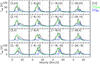 |
Fig. 4 Mon R2 [O I] 63 μm, [O I] 145 μm, and [C II] mosaic spectra for the central area of the source. The dotted lines are located at 5, 10, 15, and 20 km s−1, respectively. The angular resolution is the same for [C II], [O I] 145 μm and [O I] 63 μm (15″), with a grid spacing of 10″. The offset coordinates of each spectrum with respect to the source position are given in the top-left corner of each box. |
Mon R2 and M17 SW [O I] 145 μm and [O I] 63 μm integrated and peak intensity.
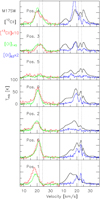 |
Fig. 5 Same as Fig. 3, but for M17 SW. The dotted lines mark the two absorption dips present for both fine structure lines at 21 and 24 km s−1. |
Mon R2 and M17 SW background excitation temperatures for both transitions and their respective kinetic temperatures.
4.1 Fitting the background emission
The observed line profiles are then fitted by a two-layer model with a background in emission (b) composed of several components (Nb) and an absorbing foreground (f) with a different number of components (Nf), each with the fit parameters above. As we do not know the details of the excitation of the three levels (two excitation temperatures) of the atomic oxygen fine structure level system, we used the peak main beam brightness temperature of [O I] 63 μm, shining through in between the absorption notches, for the estimation of the background excitation temperature of [O I] 63 μm by applying the inverse Rayleigh-Jeans correction. Then, we derived the background [O I] 145 μm excitation temperature via the analytic solution to the balance equation between collisional excitation and de-excitation with spontaneous emission. We refer to Appendix B for a detailed description of the procedure. The outcome is almost independent of the assumed density. The resulting kinetic temperatures in the background layer are given in Table 3 for a density of 106 cm−3. In Sec. 5 we further investigate how sensitive the derived column densities of the background and foreground layers are against variations of the assumed density and kinetic temperature of the background layer.
The kinetic temperatures for the atomic oxygen derived in this way are in the temperature regime expected for PDR-gas, heated by the photo-electric effect well beyond the substantially lower dust temperature in the PDR material. For the dust, Rayner et al. (2017) and Schneider N. (priv. comm.) have derived for Mon R2 and M17 SW, respectively, dust temperatures below 30 K (see a comparison between gas and dust results in Sec. 5.4). The CO rotational lines, particularly in the mid-J transitions, trace warm molecular gas from the PDR in a similar temperature range as we have derived here for atomic oxygen. Higher kinetic temperatures than the ones given in Table 3 are possible; their impact on the derived column density of the background is explored in Sec. 5.1.
We started with the fit of the observed [O I] 145 μm line profiles. First, we fit the background emission in the [O I] 145 μm line profile by several emission line background components composed of a Gaussian optical depth profile scaled by the R-J correction. The excitation temperature was fixed to the common value, ![Mathematical equation: $\[T_{\mathrm{ex}_{b, 145}} \equiv T_{\mathrm{ex}_{145, b q}}\]$](/articles/aa/full_html/2024/10/aa50530-24/aa50530-24-eq20.png) , as discussed above. The fit parameters are the upper state column density of each background component b,
, as discussed above. The fit parameters are the upper state column density of each background component b, ![Mathematical equation: $\[N_{u_{145}, b}\]$](/articles/aa/full_html/2024/10/aa50530-24/aa50530-24-eq21.png) , their LSR velocity υLSR,b, and their line width Δυfwhm,b, using the lowest possible number of Gaussian components. We note that a higher number of Gaussian components will not increase the total column density. Thus, there is no reason to use more components than needed. The process is iterative and we increased the number of components one by one until there is no substantial decrease in the chi-square of the fit with additional components. Then, we stopped the iteration. In this way, the simple, nearly Gaussian profiles of [O I] 145 μm require one or two components, B = B145, for the fitting.
, their LSR velocity υLSR,b, and their line width Δυfwhm,b, using the lowest possible number of Gaussian components. We note that a higher number of Gaussian components will not increase the total column density. Thus, there is no reason to use more components than needed. The process is iterative and we increased the number of components one by one until there is no substantial decrease in the chi-square of the fit with additional components. Then, we stopped the iteration. In this way, the simple, nearly Gaussian profiles of [O I] 145 μm require one or two components, B = B145, for the fitting.
Next, we identified the contribution of these B145 components to the line wing emission of the lower transition, [O I] 63 μm. The [O I] 63 μm upper-level column density is fixed at the value derived from the upper state column density of the [O I] 145 μm line, converted using the excitation temperature of the background via the Boltzmann-relation (Eq. (4)). The line center position, υLSR,b, is also fixed within a narrow range (10% of the value) for each component, namely to the value fitted for the [O I] 145 μm profile, and the [O I] 63 μm excitation temperature is fixed to the value of ![Mathematical equation: $\[T_{\mathrm{ex}_{63, b g}}\]$](/articles/aa/full_html/2024/10/aa50530-24/aa50530-24-eq22.png) derived above. The fit results show that the fitted width is typically less than 10% smaller for the [O I] 63 μm line, and thus consistent with the width fitted for the upper line. The fitting is restricted to the [O I] 63 μm line wings not affected by foreground absorption; the relevant velocity ranges are from 2 to 5 and 14 to 18 km s−1 for Mon R2 and from 12 to 15 and 25 to 28 km s−1 for M17S SW respectively.
derived above. The fit results show that the fitted width is typically less than 10% smaller for the [O I] 63 μm line, and thus consistent with the width fitted for the upper line. The fitting is restricted to the [O I] 63 μm line wings not affected by foreground absorption; the relevant velocity ranges are from 2 to 5 and 14 to 18 km s−1 for Mon R2 and from 12 to 15 and 25 to 28 km s−1 for M17S SW respectively.
These fitted [O I] 63 μm line profiles, resulting from the b = 1... B145 background components, show (outside of the core emission, which is heavily blended with the self-absorption) weak fit residuals requiring B63 additional background velocity components, which we number by b = B145 + 1,..., B145 + B63. We fit these by fixing the excitation temperature to the value used for the background emission. However, we can allow the column densities of the additional [O I] 63 μm emission components, ![Mathematical equation: $\[N_{u_{63}, b}\]$](/articles/aa/full_html/2024/10/aa50530-24/aa50530-24-eq23.png) , to vary freely, as well as their line widths and central velocities, ΔυFWHM,b, υLSR,b. These components are not visible in [O I] 145 μm due to their low column density derived from the fit. This effect can be verified by calculating the corresponding [O I] 145 μm background emission, which turns out to be of the order of 0.1 K or lower. We followed a step-by-step procedure instead of simultaneously fitting both [O I] lines because the weak background components are only visible in [O I] 63 μm, while the main components come from [O I] 145 μm. Therefore, we did not expect a one-to-one correlation between the two [O I] lines.
, to vary freely, as well as their line widths and central velocities, ΔυFWHM,b, υLSR,b. These components are not visible in [O I] 145 μm due to their low column density derived from the fit. This effect can be verified by calculating the corresponding [O I] 145 μm background emission, which turns out to be of the order of 0.1 K or lower. We followed a step-by-step procedure instead of simultaneously fitting both [O I] lines because the weak background components are only visible in [O I] 63 μm, while the main components come from [O I] 145 μm. Therefore, we did not expect a one-to-one correlation between the two [O I] lines.
The total column densities of oxygen are listed in Table 4, obtained from the upper and lower [O I] transitions derived from fitting the background emission profiles for the [O I] 145 μm transition (background only) and the [O I] 63 μm transition. These column densities are obtained by adding up all velocity components; however, the total column density is dominated by the one to two components b = 1 ... B145 dominating the [O I] 145 μm emission. We note that the detailed fit parameters of all components and levels are listed in DOI:10.5281/zenodo.13800536.
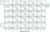 |
Fig. 6 M17 SW [O I] 63 μm, [O I] 145 μm, and [C II] mosaic. The two dotted vertical lines per spectrum are located at 22 and 24 km s−1, respectively, added to guide the eye to the absorption dips. The upper left corner in each box gives the offsets of each spectrum. |
Mon R2 and M17 SW [O I] 145 μm and [O I] 63 μm background column density per position for the two layer model.
4.2 Fitting of the foreground component
In the next step, we dealt with the foreground absorption visible in the [O I] 63 μm line. The column densities of the foreground absorption components are derived by fitting the absorption profiles against the fitted line profile of the [O I] 63 μm background emission. The intensity in the self-absorption notches drops to very low values. This intensity requires correspondingly low [O I] 63 μm excitation temperatures of the absorbing material. Due to the high energy of the [O I] 63 μm transition, the resulting optical depth hardly depends on the exact value of Tex. As we do not have a way to independently derive a value of the excitation temperature of the foreground material, we fix the foreground excitation temperature to a single and low value of ![Mathematical equation: $\[T_{\mathrm{ex}_f}=20 \mathrm{~K}\]$](/articles/aa/full_html/2024/10/aa50530-24/aa50530-24-eq26.png) . The population of the [O I] 63 μm upper level is very small at these low excitation temperatures, so the total column density is also very insensitive to the assumed, fixed
. The population of the [O I] 63 μm upper level is very small at these low excitation temperatures, so the total column density is also very insensitive to the assumed, fixed ![Mathematical equation: $\[T_{\mathrm{ex}_f}\]$](/articles/aa/full_html/2024/10/aa50530-24/aa50530-24-eq27.png) . In Sec. 5.1 we verify this weak sensitivity of the fitted foreground column density on the exact value of the assumed value of
. In Sec. 5.1 we verify this weak sensitivity of the fitted foreground column density on the exact value of the assumed value of ![Mathematical equation: $\[T_{\mathrm{ex}_f}\]$](/articles/aa/full_html/2024/10/aa50530-24/aa50530-24-eq28.png) . Because of the low excitation temperature of the [O I] 63 μm transition, the [O I] 63 μm upper level, providing the lower level of the [O I] 145 μm transition, is hardly populated so that the foreground does not contribute to the observed [O I] 145 μm line profile at all; neither in emission nor in absorption, independent of its assumed excitation temperature. Therefore, the foreground fit is done to the [O I] 63 μm profile alone. This approach is backed up by the lack of self-absorption nodges in the observed [O I] 145 μm line profile.
. Because of the low excitation temperature of the [O I] 63 μm transition, the [O I] 63 μm upper level, providing the lower level of the [O I] 145 μm transition, is hardly populated so that the foreground does not contribute to the observed [O I] 145 μm line profile at all; neither in emission nor in absorption, independent of its assumed excitation temperature. Therefore, the foreground fit is done to the [O I] 63 μm profile alone. This approach is backed up by the lack of self-absorption nodges in the observed [O I] 145 μm line profile.
With the excitation temperature fixed to this low value, this leaves the foreground column densities, ![Mathematical equation: $\[N_{l_{63}, f}\]$](/articles/aa/full_html/2024/10/aa50530-24/aa50530-24-eq30.png) , line width, ΔυFWHM,f, and line center, υSR,f, as the fitting parameters of the foreground components. As the [C II] and [O I] absorption dips are very similar in line center velocity and width, we use the line center position and width of the [C II] foreground components fitted by Guevara et al. (2020) as initial guesses for the foreground [O I] fitting of the most substantial absorption components. We keep the velocity of the [C II] components fixed, allowing for a minor variation in width, and we freely vary the oxygen column density. An example of the fitting is shown in Fig. 7, which shows the results for position 2 in Mon R2 for both [O I] lines. The thus fitted column densities of the foreground are listed in Table 5.
, line width, ΔυFWHM,f, and line center, υSR,f, as the fitting parameters of the foreground components. As the [C II] and [O I] absorption dips are very similar in line center velocity and width, we use the line center position and width of the [C II] foreground components fitted by Guevara et al. (2020) as initial guesses for the foreground [O I] fitting of the most substantial absorption components. We keep the velocity of the [C II] components fixed, allowing for a minor variation in width, and we freely vary the oxygen column density. An example of the fitting is shown in Fig. 7, which shows the results for position 2 in Mon R2 for both [O I] lines. The thus fitted column densities of the foreground are listed in Table 5.
We note that a few Gaussian components have narrow line widths below 1 km s−1. These narrow components are located at the wings of the other narrow absorption dips. They are necessary for the fit to match the non-Gaussian absorption profiles. We do not regard them as independent physical components. They all have small amplitudes and, thus, we added their correspondingly small column densities to the column densities of the adjacent components.
Mon R2 and M17 SW [O I] 63 μm foreground column density per position for the two-layer model.
4.3 Foreground and background column densities
The derived total column density of the [O I] background and foreground, given by the sum of the individual velocity components, are listed in Tables 6 and 7, respectively. For easier comparison, the column densities are also converted to hydrogen column densities, NH, and to equivalent visual extinctions, assuming that all oxygen is in the form of O0. From Wakelam & Herbst (2008, their table 1, for high-metal elemental abundances), we use an O/H abundance ratio of 2.56 × 10⁻⁴. We consider the canonical conversion factor between the total hydrogen column density and visual extinction of 1.87×1021 cm−2/AV (Bohlin et al. 1978). Tables 6 and 7 also compare the total oxygen column densities of the foreground and background components to the ones derived previously for [C II]. The C+ column density also has been converted to an equivalent visual extinction using a C/H abundance value from Wakelam & Herbst (2008, same as above, table 1) of 1.2×10⁻⁴ and the canonical conversion factor listed above to convert to magnitudes. The tables also list the ratio of the [O I] and [C II] column densities and the ratio of the equivalent extinctions. The abundance ratio between oxygen and carbon is 2.1 when using the elemental abundances relative to hydrogen quoted above.
To ease the visualization of the multiple foreground and background components, both for the new [O I] and the former [C II] data and, in particular, also for the discussion of the position-to-position variations below (see Sec. 5.3), we compared the fitted parameters for different components in the foreground and background; namely, their velocities, velocity widths, and column densities, in Figs. 8 and 9
We notice that the background column density ratio of [O I] to [ C II] is close to the elemental abundance in most positions; correspondingly, the equivalent AV ratio is close to unity. This ratio is expected if all material is fully excited. However, due to the higher critical density of the [O I] transitions, it is likely that more C+ is traced in emission. Therefore, we would expect to measure a background column density ratio between oxygen and ionized carbon, where the elemental abundance is the upper limit. However, the value for Mon R2, position 1, in the background layer, clearly sticks out; the other two cases for an [O I] excess in the background layer well above the elemental ratio are positions 1 and 5 in M17 SW. We note that for these positions, we use a relatively low ![Mathematical equation: $\[T_{\mathrm{ex}_{63, b q}}\]$](/articles/aa/full_html/2024/10/aa50530-24/aa50530-24-eq31.png) , derived from the relatively low peak brightness of the [O I] 63 μm line. The latter is a lower limit, which holds in the optically thick case; higher values for Tex are perfectly feasible and would result in a correspondingly lower [O I] column density, as discussed in Sec. 5.1. On the other hand, positions 0, 4, and 6 for M17 SW have a lower oxygen column density than the other positions. As discussed above, these values could be an effect of a too-low density of the collision partners to excite the oxygen; see Sects. 5.1 and C.1 for an explanation of how density affects the results.
, derived from the relatively low peak brightness of the [O I] 63 μm line. The latter is a lower limit, which holds in the optically thick case; higher values for Tex are perfectly feasible and would result in a correspondingly lower [O I] column density, as discussed in Sec. 5.1. On the other hand, positions 0, 4, and 6 for M17 SW have a lower oxygen column density than the other positions. As discussed above, these values could be an effect of a too-low density of the collision partners to excite the oxygen; see Sects. 5.1 and C.1 for an explanation of how density affects the results.
For the foreground layer, we expect an opposite situation. In cold material, some atomic oxygen may be left in the overall molecular material where most carbon is bound in CO. Therefore, we should measure a [O I] to [C II] abundance ratio higher than the elemental abundance in absorption. Mon R2 presents the higher ratios for both sources. Given the likely scenarios for the structure of Mon R2 (see Sec. 5.3), it is expected that this excess is due to the inherent structure of the source. M17 SW shows a different behavior. The values that deviate from what is expected are found in positions 0, 2, 4, and 6.
Interestingly, the affected positions are closer to the main ridge (see Fig. 2). It is clear that a particular spatial configuration plays a role here. However, with the foreground layer being invisible and only being detected through the absorption profile of bright atomic lines, it is hard to speculate without much information. Future studies over the whole map for the foreground layer in both lines could help to resolve this issue.
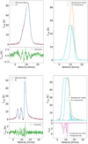 |
Fig. 7 Mon R2 [O I] fits for position 2 for both transitions. The background fit needs 7 components, the 2 coming from the [O I] 145 μm line carrying the bulk of the column density, plus 5 additional weak ones. The foreground fit needs 6 components. Top: Mon R2 [O I] 145 μm fitting for position 2. Top left: This panel represents the fitted model in blue and the observed spectra in red. Bottom left: residual curve between the observed spectra and the model. Right: composition of each fitted component in cyan. Bottom: Mon R2 [O I] 63 μm fitting for position 2. Top left: fitted model in blue and the observed spectra in red. Bottom left: residual curve between the observed spectra and the model. Top right: composition of each fitted component in cyan and the fitted [O I] 63 μm background profile in orange. Bottom right: foreground optical depth for the [O I] 63 μm line of each Gaussian component in pink. |
5 Discussion
We have estimated the background and foreground column densities for neutral atomic oxygen under the assumption of a lower limit for the excitation temperature in the background layer along the line of reasoning discussed in Appendix B. With the estimated range of excitation temperatures for [O I] 63 μm between 65 and 145 K, we derive column densities from the fit to the observed line profiles between 8.5 and 49 × 1018 cm−2 for the background layer and between 1.8 and 4.6 × 1018 cm−2 for the foreground layer. In the following, we first evaluate how sensitively the results are affected by the necessary simplifying assumptions we made. Then, we turn to a discussion of the characteristics of the foreground layer.
5.1 Effect of variations in the background and foreground physical parameters
The choice of the value for the excitation temperature of the background layer in both [O I] transitions is a critical element of the study, as the temperature in the foreground layer. As presented above, we have taken the excitation temperature of the [O I] 63 μm transition in the background as the lower limit derived from the peak brightness temperature of this transition observed at each position; with the assumption of high density, necessary because of the high critical density of the [O I] 145 μm transition, we then use the analytical solution for the population of the three-level [O I] fine structure system (see Appendix B) to derive the excitation temperature for the upper transition (assuming 106 cm3 for the density). To estimate how sensitive the derived column densities for the background layer components are to these assumptions, we analyzed how the result depends on varying first the density (see Appendix C.1), then on the kinetic temperature of the background components (see Appendix C.2).
This analysis shows that the resulting background column densities span a range in physical scenarios of warm PDR material with correlated temperatures; they can reach about ten times larger column densities for the background compared to the minimum derived for the nominal parameters. Thus, from this analysis alone, the amount of warm PDR material traced by the atomic oxygen background emission cannot be constrained further but is in a range entirely consistent with standard PDR scenarios and also with the range of column densities for warm PDR gas traced by mid- and high-J CO lines (for example, Stutzki et al. 1988; Pilleri et al. 2012; Pérez-Beaupuits et al. 2015a).
Finally, we vary the foreground excitation temperature and study its effects on the derived foreground column density (see Appendix C.3). The foreground excitation temperature analysis shows that the column density is not much affected by the assumed value for the foreground excitation temperature, changing monotonically by not more than 20% over the possible temperature range. Thus, we conclude that the foreground column density of the absorption components, derived from the fit to the complex line profiles, is a robust result.
Mon R2 and M17 SW comparison between oxygen and ionized carbon column densities and equivalent extinctions for the background columns.
Mon R2 and M17 SW comparison between oxygen and ionized carbon column densities and equivalent extinctions for the foreground columns.
5.2 Column densities of the different components of the background layer
One of the central motivations behind this work is to study the nature of the foreground layer identified through the self-absorption traced by both cooling lines, [C II] and [O I]. Nevertheless, we also briefly discuss the nature of the background layer. In Fig. 8, we plot the column density for each fitted Gaussian velocity component for both [C II] and [O I] for each position analyzed. [C II] is characterized by diamonds and [O I] by circles.
One or two components dominate the background column density contribution for both atoms around the systemic velocity, 10 km s−1 for Mon R2 and 21 km s−1 for M17 SW with more than 80% of contribution from these main components. We also see that the additional components tracing the line wings contribute only marginally to the column density, with Mon R2 showing a red-shifted line wing and M17 SW showing emission at both sides skewed to the blue side of the spectra.
We notice that the main background emission, both in [C II] and in [O I], is fitted by a few well-overlapping Gaussian components, resulting in a smooth overall profile. Sometimes even only one single component dominates, in particular in [C II], where the bulk background emission is defined by the [13C II] line profile. The [O I] background emission, having to match both the [O I] 145 μm profile and the line wings of heavily self-absorbed [O I] 63 μm profile, sometimes requires several more Gaussian components; these are, however heavily overlapping and sum-up to a similar total column density than the single [C II] component (one example is the three components at M17 SW pos. 0, or the two components in [O I] matching the single component in [C II] at M17 SW pos. 3).
Nonetheless, the dominant contribution in column density comes from components where both are present and which have similar velocities and line-width in [C II] and [O I]. We can see that the background is not entirely uniform and shows some variations from position to position. To conclude, the background, at the different positions, shows a smooth line structure dominated by one or two Gaussian components and consistent velocities around the systemic velocity.
We also note that the center velocities and line widths of ionized carbon and atomic oxygen are similar to the emission observed in other tracers, such as atomic carbon and carbon monoxide. For Mon R2, the emission spans a range between 0 and 20 km s−1, with a peak intensity around 10 km s−1, not different from what we see in other tracers such as CO (e.g. Pilleri et al. 2012); however, the CO emission shows much more complex line profiles with additional foreground absorption. The same is the case for M17 SW if we compare the emission to observations in [C I] or CO, in particular, for the optically thin lines Pérez-Beaupuits et al. (2015a,b), with emission between 10 and 30 km s−1 and their intensities peaking around 20 or 22 km s−1, plus additional components outside this velocity range mentioned above, only visible in [C II].
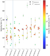 |
Fig. 8 Compilation of background Gaussian parameters for all positions from the multi-component analysis from Sec. 3. Each position is plotted in columns along the velocity axis, showing both atomic lines. Circles symbolize the [O I] Gaussian components for each position and triangles the [ C II] ones (from Guevara et al. 2020). The color of each symbol represents its column density. The length of the vertical bars denotes half of the line width value for a better visualization. |
5.3 Physical properties of the foreground layer
The significant result from the previous observations and analysis (Guevara et al. 2020) of the [C II] self-absorption notches was that they require a large foreground column of [C II] with very low Tex material (≤20 K). The present study shows that the [O I] 63 μm line also shows deep self-absorption notches, which generally agree well in terms of velocity and line width with the [C II] self-absorption when both are present and correspond to similar total column densities.
Similarly to the background emission components analysis shown in Fig. 8, we display the column densities, velocities, and line widths of the individual foreground components in Fig. 9. The figure demonstrates that the self-absorption notches in [C II] and [O I] 63 μm have similar velocities and narrow line widths. Moreover, the different components at the other positions can be grouped around common velocities, with 8 and 12 km s−1 for Mon R2, and 16, 18, 21, and 24 km s−1 for M17 SW. However, the exact velocity for each component fluctuates around these average values, the magnitude of these fluctuations being on the order of the line widths.
The total column density at each position is distributed between different velocities, and the column density of a given velocity component varies from position to position. As discussed above, most velocity components in the foreground are seen in both species, [O I] and [C II], with similar fit parameters. In several cases, the foreground absorption, being fitted by a single component in one species, requires two velocity components with different widths in the other. Some examples are M17 SW, pos. 0, where the [O I] 63 μm absorption at 24.1 km s−1 is fitted by a single component with a width of 0.6 km s−1, whereas the corresponding [C II] absorption at 24.1 km s−1 needs two components: one with a wider line width of 2 km s−1 and a narrower one with a width of also 0.6 km s−1. A similar situation is shown for the 21.3 km s−1 center velocity component in M17 SW, pos. 3, where the [C II] absorption is fitted by a single component of width 2.2 km s−1 (Table F.4 in Guevara et al. (2020)) and the [O I] absorption needs two fit components, one with width 2 km s−1, the other one with a with of 1.1 km s−1. These differences are presumably due to the oversimplifying assumption of purely Gaussian absorption line profiles; the different fit components, nevertheless, can safely be counted as contributions to the same absorption feature.
It is solely on very few occasions that an absorption component appeared only in [O I]and not in [C II]. This phenomenon only occurs in the line wings and for features with relatively low column density; examples are the 25.9 km s−1 and the 16.9 km s−1 component in M17 SW, pos. 3, or the 15.5 km s−1 component in M17 SW, pos. 6. In all these cases, the significance of the absorbing foreground fit components may be spurious, as the absorption is fitted against the weak and somewhat noisy line wings of the background [O I] 145 μm emission line profiles.
In contrast, there are several cases where the [C II] line shows clear absorption components but where the corresponding [O I] 63 μm absorption shows much lower column densities or is almost absent. This absorption is typically the case for the [C II] absorption on the low-velocity side of the line profiles in M17 SW. Examples are the 16.4 and 19.1 km s−1 components at pos. 0, see Table F4 in Guevara et al. (2020), and the corresponding [O I] 63 μm absorption component at 17.4 km s−1, or the 16.6 and 19.9 km s−1 [C II] components in pos. 4 (see Table F4 as above) and the corresponding [O I] 63 μm component at 19.6 km s−1. As the [O I] emission does not show the weak wing emission below 17 km s−1, these features cannot show up in absorption in [O I] 63 μm, even if they might be present in the foreground, as they lack background emission to absorb against.
Both cases discussed above occur in the wings of the main line emission. The quantitative comparison of [O I] and [C II] column densities in these components might be affected by the slightly different form of the emission line profiles from the background. Similarly, the quantitative comparison of the absorbing column densities from position to position, as discussed in the next paragraph, will be affected by the features in the line wings by corresponding variations in the line profile of the background emission.
5.3.1 Spatial variations and density estimate
We can obtain a lower limit estimate for the density of the foreground material from the variations in the derived foreground column density between adjacent positions. To illustrate the range of densities and spatial scales involved, let us, for the moment, assume a diffuse foreground of density 100 cm−3, already relatively high for a diffuse cloud. The atomic oxygen column densities derived for the foreground of around 2 × 1018cm−3 (Table 7) together with the oxygen abundance quoted above would then imply a spatial extent along the line of sight of 7.8 × 1019cm. Taking this as the typical size of the assumed homogeneous foreground cloud would imply an angular extent of 45 arcmin (~30 pc) at the distance of M17 SW.
Based on the larger uncertainties for the derived column density values of the foreground absorption against the background line wings, as discussed above, we focus on the analysis of the variation in column density of the foreground components from position to position, on the absorbing components in the line cores, which are less affected by the uncertainties in the background brightness, namely the features at velocities between 18 and 25 km s−1. Comparing the absorption feature near 24.1 km s−1 ¸ at pos. 0 and pos. 1 of M17 SW, namely, between a position on the bright interface ridge to one further into the molecular cloud, which has a total H I-equivalent column density of 2.8 × 1021 cm−2 at pos. 0 and drops to 0.8 × 1021 cm−2 at pos. 1; hence, it shows a decrease by 2.0 × 1021 cm−2 in [C II], and from 4.5 × 1021 cm−2 to 0.6 × 1021 cm−2, and, therefore, a decrease of 3.9 × 1021 cm−2 in [O I]. Comparing the column density variations between positions along the ridge (i.e pos. 3 and pos. 0), the velocity components at about 21.3 to 21.7 km s−1 drop in [O I] from (3.5 + 0.6 × 1021 cm−2) to 2.0 × 1021 cm−2¸ (i.e., a 2.1 drop), whereas it increases from 4.2 to 6.2, namely, an increase of 2.0 in [C II]. The rise in [C II] versus the decrease in [O I] in this case indicates a change in the chemical composition along the line of sight from position to position. Repeating this comparison for all pairs of adjacent positions, we see that the variations from position, both in [O I] and [C II], are typically of the order of 1 to 2 × 1021 cm−2 and peak variations are up to about 4 × 1021 cm−2. This comparison includes the variations in column density between the two positions measured in Mon R2.
To understand to what degree the variations in the absorbing column densities from position to position might be an artifact of the ambiguity of the foreground absorption fit with several Gaussian components, we checked how the resulting fitted line profile looks like if we fix the foreground components to the parameters from the adjacent position, first in all three foreground line parameters: line center, width, and column density. We have done this test for position 1 in Mon R2 with the parameters of position 2 and position 6 in M17 SW with the parameters of position 0. As an example, Fig. 10 shows the resulting fit for M17 SW position 6. In a second test, we allowed each foreground component’s column density and line width to vary, keeping the velocity (and excitation temperature) fixed (Fig. 11 shows an example of the resulting fit). Both attempts are unsuccessful, as demonstrated by the significant residuals well above the noise level, with (obviously) slightly better results, allowing for more variations. Considering that the foreground absorption is multiplicative, ![Mathematical equation: $\[e^{-\tau_{f g}}\]$](/articles/aa/full_html/2024/10/aa50530-24/aa50530-24-eq36.png) , implying that the optical depth is determined as a proportion of the background intensity and hence independent of its actual intensity and background intensity variation, this demonstrates that the variation in column density, and therefore optical depth, between adjacent positions derived from the complete fits of the two-layer model as discussed above, is a significant result. Keeping the column density constant across adjacent positions, as would be the case for a smooth and homogeneous foreground component, contradicts the observed line profiles.
, implying that the optical depth is determined as a proportion of the background intensity and hence independent of its actual intensity and background intensity variation, this demonstrates that the variation in column density, and therefore optical depth, between adjacent positions derived from the complete fits of the two-layer model as discussed above, is a significant result. Keeping the column density constant across adjacent positions, as would be the case for a smooth and homogeneous foreground component, contradicts the observed line profiles.
Thus, we derived the variations in H I equivalent column density for each species to be between 1 and 2 and up to 4× 1021 cm−2. These are variations of the total column density, such as a decrease or increase in both species, or they indicate the variation of the chemical composition along each line of sight, in case the variation is in the opposite sense for both species. The linear scales between adjacent positions correspond to 0.27 pc at the distance of M17 SW and 0.12 pc for Mon R2.
As discussed in Guevara et al. (2020), assuming that the components observed are not all pencil-like directed along the line of sight, the magnitude of the column density variation, combined with the linear scale corresponding to the angular separation at the distance of the source, gives a constraint on the variation of the density of the foreground material and, hence, a lower limit estimate of the density of the foreground material. With the numbers quoted above, this results in minimum hydrogen volume densities of 1.2–2.4 × 103 cm−3, maximum about 5 × 103 cm−3 for M17 SW, and correspondingly higher, according to the closer distance and hence smaller linear scale between the observed positions, namely, 2.8–5.6 × 103 cm−3, for Mon R2.
We emphasize that these densities are a lower limit due to several factors: first, the densities are derived from beam-averaged column densities. Thus, if the source has structure on scales smaller than the beam, the column densities, and hence the derived densities, will be accordingly higher. Secondly, the densities are derived from the smallest observed distance, the pixel spacing of the upGREAT array; similar changes on smaller scales, as suggested by the profile changes shown for the fully sampled [C II] map and the regridded [O I] map in Fig. 6 would give correspondingly larger densities. In addition, the densities can be higher if the absorbing material is a surface layer significantly smaller than the spatial size of the variations. And lastly, the derivation of the H I column densities assumes that all the material is in the form of O0 and C+; they would be correspondingly higher, and similarly for the volume densities, if only a fraction of the material is in the form of O0 or C+, a possibility that is already indicated by the variation of the O0 and C+ column density ratios for the different components and positions. The lower limit for the density of the absorbing foreground derived in this way, estimated from the variation in column density from position to position, is two to three orders of magnitude greater than typical for homogeneous diffuse absorbing foreground layers.
As a side note, we can estimate the kinetic temperatures for these densities that would result in the excitation temperature we have used for our analysis, 20 K, from the excitation temperature plots in Appendix B. This estimation gives a foreground kinetic temperature of 30 K for Mon R2 and 38 K for M17 SW. The total column density of the low Tex, absorbing foreground, is very large as shown in Table 7, corresponding to an equivalent visual extinction of several AV or more. The agreement in velocity implies that it is associated with the source. Based on the arguments above about the spatial (in projection) variation of the derived column densities, we estimate it to have a relatively high density. Both the column and the volume densities are lower limits, assuming that all its carbon is in the form of C+ and all its oxygen is in the form of O0. These arguments strongly suggest that the material is not a diffuse, smooth foreground layer but is directly associated with the background material, namely, the dense, strongly UV-illuminated PDR material.
The nature and origin of this material are somewhat puzzling: we would need a mechanism that produces such a large column of low Tex, dense material, but where the carbon stays ionized although the high density should favor rapid recombination, as is firmly predicted by PDR scenarios. At the same time, the oxygen remains in atomic form despite the significant extinction and high density that would tend to transform O0 to CO, depleting all the available carbon and also forming OH or H2O.
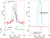 |
Fig. 10 Unsuccessful (note the significantly increased level of the residuals) fit for M17 SW pos. 6, using the foreground parameters fitted to position 0. |
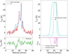 |
Fig. 11 Same as Fig. 10, using the foreground parameters fitted to position 0, but allowing for variations in width and column density. |
5.3.2 Chemical composition
Assuming that carbon might be only partially ionized, with a part as neutral atomic carbon or in a molecular form such as CO, would increase the amount of material not visible in any other tracer. In parallel, additional oxygen would have to be present in molecular form, presumable water ice, frozen out on dust. The attractive scenario of putting the extra carbon and oxygen into carbon monoxide can be ruled out observationally, as the low-J CO lines, in particular, those from rare isotopologues do not show a comparable column of cold CO. This analysis holds for the positions in M17 SW (Pérez-Beaupuits et al. 2015a), where the O0 and C+ column densities are consistent with the elemental abundances.
For the positions where the derived column density ratio of oxygen to carbon is higher than the elemental abundance (i.e., positions 3 and 5 in M17 SW and both positions in Mon R2), we can assume that carbon in the foreground absorbing material is indeed only partially ionized, with a fractional ionization of 20–50%. Alternatively, the absorbing layer may be composed of two chemically different components, where a column density of about 20–50% of the total would have to be low Tex, fully ionized [C II] material. For the Mon R2 lines of sight, the assumption of additional absorbing material is perfectly reasonable. It is known that Mon R2 is an embedded source with several young stellar objects (YSO, Beckwith et al. 1976) inside the molecular cloud illuminated from the backside. This darkening could help to explain the large discrepancy between the O0 and C+ column densities, compared to M17 SW, but does not explain the correlation between the [O I] and [C II] emission, because we would not expect the presence of ionized carbon in the dense molecular foreground material. Pilleri et al. (2012) proposed in their model for Mon R2, apart from the dense PDR, a surrounding envelope with densities of 5× 104 cm−3, molecular hydrogen column density of 5× 1022 cm−2 and kinetic temperature of 35 K, similar values that we find here for the foreground layer and its estimated density from the differences between positions, confirming our results. Hence, we have for Mon R2 a foreground separated in two phases, with a temperature gradient, where one part of the gas contains only O0 coexisting with molecular material. In contrast, in the other, outer layer O0 and C+ coexist.
M17 SW shows a different picture. The foreground column density ratios between [O I] and [C II] are lower than the elemental ratio inside the main ridge and higher outside, showing some spatial correlation playing a role. As discussed in Sect 4.3, studies over the whole map are needed. Single pointings are insufficient for a proper analysis of spatial effects. Moreover, Hoffmeister et al. (2008) found an optical foreground extinction of 2 mag, a significantly lower value than the foreground layer derived here. Therefore, we propose a scenario of a dense atomic foreground layer where ionized carbon and oxygen coexist with a density of 103 cm−3, not ruling out the existence of a density gradient towards the exterior, leading to an additional atomic diffuse layer.
Mon R2 and M17 SW dust equivalent extinction comparison.
5.4 Comparison between gas and dust
We compare the column densities derived above from the [O I] and [C II] fine-structure lines for the background and foreground components with the total gas column densities derived from the sub-mm-wavelength dust emission. The column density maps were derived from Herschel/PACS and SPIRE (Griffin et al. 2010) 250, 350, and 500 μm for Mon R2 (Rayner et al. 2017) and M17 SW (Schneider, N., priv. comm.), using the method described by Palmeirim et al. (2013). The method estimates the total gas column density from the optically thin dust emission for both sources (Table 8) by fitting the spectral energy distributions (SEDs) and computes the gas surface density distribution of the region pixel by pixel. Note that this method deals with only a single temperature component of the dust emission and is thus biased towards the bulk column density of the lower temperature gas of the molecular clouds. It also traces parts of the warm PDR material, which has bright dust emission, but the analysis weighted it down by constraining the dust emission wavelength bands to longward of 160 μm. Also, the values estimated are upper values in a 18″ beam because there is line-of-sight contamination, with AV ~ 10 mag for M17 and AV ~ 2 mag for Mon R2 (Schneider et al., in prep.).
For M17 SW, the gas column densities are between 54 and 336 magnitudes. Background equivalent extinction values derived from [O I] at all positions are beween one and ten times smaller than the ones derived from dust. This difference is unsurprising as the dust emission also traces the dense molecular material of the bulk molecular cloud. The warm PDR traced by the background emission in the fine structure lines contributes 10–25% of the total column density traced by the dust emission (Table 8). We also note that the column density of the warm PDR background derived here is larger than the one derived from the mid-and high-J CO lines (Harris et al. 1987; Pérez-Beaupuits et al. 2015a) and quoted in previous studies of the [C II] emission (Stutzki et al. 1988). The low-velocity resolution of the last [C II] observations ignored that the foreground absorption significantly weakens the [12C II] emission. We note that the cold and dense molecular cloud material responsible for the bulk dust emission is not traced by the column densities derived from the [O I] lines observed in emission. This disparity is plausible as oxygen will be mainly in molecular form (CO, H2O) and partially frozen out onto dust grains.
For Mon R2, the situation is different. The equivalent extinctions derived from dust for both positions are much closer to those derived from the [O I] fine structure lines. This closeness could be interpreted as neutral oxygen that coexists with dense foreground molecular material, as has been suggested before by several authors (Pilleri et al. 2012; Ginard et al. 2012; Treviño-Morales et al. 2019). As discussed above in Sect 5.3, the dust strengthens the scenario of a double-layered foreground, with a molecular component and another in atomic form.
The comparison of the column densities derived for the emission from the warm background in [C II] and [O I] shows that both are consistent with the emission originating in standard PDR material, with excitation temperatures between 60 and 140 K for the [O I] and between 150 and 250 K for the [C II]. As discussed in our previous analysis, the amount of material is significantly larger than expected for a single PDR layer, so we have to invoke multiple PDR layers within the beam with several tens of magnitudes in Aυ. The column densities derived here refer only to the bright PDR material in the fine structure line emission. A portion of the warm, dense PDR material will contribute to the mid- and high-J CO emissions. These lines can trace the material because we have worked under the assumption that all [O I] emission is in the form of atomic material, not considering the molecular contribution.
5.5 Comparison with other models
At his point, we want to consider whether there are alternative explanations for the nature of the foreground layer. Goldsmith et al. (2021) discussed the [O I] profile toward W3, which shows strong absorption, similar to what this paper discusses. At first sight, the situation looks similar to the Mon R2 case discussed here. They found similar values for the neutral oxygen foreground column density, from 2 to 7×1018 cm−2, reinforcing the idea of a foreground layer of atomic material with similar column densities. They attribute its foreground absorption to geometry effects because the source is heated from the backside, allowing for additional oxygen in atomic form in cold molecular layers, together with CO, between the PDR and the observer. However, such a scenario cannot explain the sizeable C+ column densities together with more prominent O0 column densities at the same velocity and line width. The [C II] absorption dips, requiring a large column of [ C II] much colder than feasible in a PDR layer, rule out a scenario similar to the one discussed for W3 by Goldsmith et al. (2021). The analysis continues in Goldsmith et al. (2023), with the modeling, through the Meudon code (Le Petit et al. 2006), of the foreground layer in W3A. Their model identifies foreground hydrogen column densities of 2× 1022 cm−2, or equivalently a oxygen column density of ~5×1022 cm−2, with a density of n(H) = 250 cm−3 over a spatial extension of 26 pc. While the interpretation of the absorption profile in [O I] resulting from a smooth foreground may be a valid scenario in the case of W3A, the [O I] absorption observed in Mon R2 and M17 SW must be due to high-density material; this is based on the differences in foreground column densities between positions over small angular distances. Mapping observations in Oone are not available for W3A; hence, a decision between these two scenarios is impossible with the presently available data. In addition, a [13C II] profile with sufficient S/N is not available in the case of W3A, so the background column density of [C II] is not well constrained. W3A might behave like our sources, but maps in [O I] and [C II] would be needed to distinguish between the scenarios. Regretfully, new observations in these atomic cooling lines will not be feasible in the near future.
Kabanovic et al. (2022) presented a similar scenario for RCW120 for [C II] only. [C II] observations show correlations between the velocity of foreground components derived from a similar multi-component double-layered Gaussian analysis and atomic hydrogen absorption dips in the line profile. Through a H I self-absorption (HISA) analysis, they compared the H I absorption line profile with that of [C II]. They found correlations in line width and LSR velocity for some components. They attributed the origin of the foreground layer causing the [C II] self-absorption to diffuse and extended H I that coexists with C+. Comparison of the foreground column density between adjacent positions and at an assumed temperature of 15 K, similar to the 20 K we use (Table 1 of Kabanovic et al. 2022), show a column density difference of 0.5–1×1021 cm−2, much lower than the values we derive for M71 SW and Mon R2 in Sect. 5.3.1. Similarly, in the case of RCW120, the difference in the foreground line profile parameters between positions (Fig. 8 of the paper as mentioned earlier), namely the intensity and velocity position and width, are much smaller for RCW120, compared to the case of M17 SW and Mon R2, showing a much more homogeneous foreground than for our sources. [O I] 63 μm was observed in the source (Kabanovic, S., priv. comm.), but there is only faint emission in the southwestern area. Besides, no [O I] 145 μm observations are available, making verifying any self-absorption effects in the [O I] 63 μm profiles difficult. New observations in high-resolution S/N for oxygen lines would be needed for an analysis similar to ours.
6 Summary
The newly observed high spectral resolution observations of the [O I] 145 μm and the [O I] 63 μm lines towards M17 SW and Mon R2 show strong absorption notches in the [O I] 63 μm line and allow for a detailed multi-component Gaussian analysis, separating the emission into a background and foreground layer. The background emission is consistent with warm, dense PDR-material emission in both sources, which is well-known and characterized by many previous studies. This material shows smooth Gaussian emission profiles towards which we formerly observed intense [12C II] self-absorption in both sources and now newly detected [O I] 63 μm foreground absorption. The deep foreground self-absorption features require significant column densities of low Tex atomic oxygen in the foreground material.
Comparison of the [O I] profiles with the previously observed [12C II] and [13C II] profiles towards both Mon R2 and M17 SW show that the [O I] 145 μm emission line profiles, tracing the warm background, are entirely consistent with the [13C II] emission profiles from the background material and have similar total column densities. The intense self-absorption notches visible in [O I] 63 μm match well with the previously observed [12C II] absorption features, both in their central velocities and widths. Hence, we conclude that (for the majority) they trace the same material, which has to be very cold (in terms of excitation temperature) due to the deep absorption. The derived column densities in the absorption layer are also consistent for both species. The physical parameters of the background layer, though the column density derived can vary by a factor of up to 10 depending on the detailed assumptions, are, for both species, entirely consistent with a multi-layer PDR at the UV intensity and density of the bulk material in M71 SW and Mon R2.
The physical parameters of the foreground layer are well-constrained based on the analysis presented. The large column density of the foreground material and the small spatial scales derived from the sudden variation of the central velocity and depth of the absorption features constrain the foreground material to have a significant density between 103 and 104 cm−3. The nature of this foreground layer, with its fully ionized carbon and atomic oxygen at relatively high densities and low excitation temperature, is very puzzling.
We emphasize that the foreground absorption is only visible at the high spectral and spatial resolution available with the upGREAT instrument on SOFIA and Galactic sources. Spatial averaging, namely, observations of sources at a larger distance, namely in nearby or further out galaxies, resulting in lower spectral resolution observations, smooth out the absorption features in the line profiles, leading to reduced integrated intensity. Thus, the absorbing foreground absorption component of unidentified origin may be partially responsible for the [O I] and [C II] line intensity deficiencies quoted for such sources. Large-scale mapping observations with high signal-to-noise in both [C II] and [O I] fine structure lines and their analysis in galactic clouds are necessary to resolve this issue. We analyzed one of the best datasets that combines both [C II] isotopes with both [O I] transitions, and without access to new observations at the exact resolution and S/N in the near future, it will be hard to disentangle this scenario. Still, we can affirm without doubt that there is a cold, relatively dense foreground layer associated with the main PDR composed of ionized carbon and neutral oxygen absorbing the emission of the background.
Acknowledgements
This work is based on observations made with the NASA/DLR Stratospheric Observatory for Infrared Astronomy (SOFIA). SOFIA was jointly operated by the Universities Space Research Association, Inc. (USRA), under NASA contract NNA17BF53C, and the Deutsches SOFIA Institut (DSI) under DLR contract 50 OK 0901 to the University of Stuttgart. The work was carried out within the Collaborative Research Centre (CRC) 956 sub-projects A4 and C1 (project ID 184018867) and CRC 1601 sub-projects A6 and B2, funded by the Deutsche Forschungsgemeinschaft (DFG), project ID 500700252. This research was carried out in part at the Jet Propulsion Laboratory, California Institute of Technology, under contract with the National Aeronautics and Space Administration (80NM0018D0004). S.K. acknowledges support from the Orion-Legacy project that is supported by the BMWI via DLR, project number 50OR2311.
Appendix A Observational parameters
In this appendix, we provide the observational parameters of the observed positions in detail. The coordinates of each position are the same as the original [C II] observations from Guevara et al. (2020). The tables contain the absolute and relative coordinates (with respect to the source coordinate, see Table 1) for each observed position and their OFF position.
Monoceros R2 and M17 SW positions.
Appendix B Excitation temperature estimate for the [O I] line for the background
We have estimated the excitation temperature for both [O I] transitions in a three step process. We do not have previous information about the excitation temperature of the oxygen; therefore, as a starting point we assume that [O I] 63 μm is optically thick so that the brightness temperature traces the excitation temperature (including the Rayleigh-Jeans correction), and at least at one velocity, the background brightness temperature shines through the foreground absorption. Hence, we have selected as a lower limit for the [O I] 63 μm the Tmb peak emission and then converted to Tex given by the Rayleigh-Jeans correction under the assumption of optically thick emission as:
![Mathematical equation: $\[T_{\mathrm{mb}}=\mathcal{J}_\nu\left(T_{\mathrm{ex}}\right)=\frac{h \nu}{k}\left(e^{h \nu / k T_{\mathrm{ex}}}-1\right)^{-1}.\]$](/articles/aa/full_html/2024/10/aa50530-24/aa50530-24-eq41.png) (B.1)
(B.1)
With the excitation temperature of the [O I] 63 μm line, we can estimate the excitation temperature of the [O I] 145 μm line, though the balance between collisional excitation and de-excitation and spontaneous emission when assuming a gas density. Then, the collisional rate Cij from level i to j is given by:
![Mathematical equation: $\[C_{i j}=R_{i j} n,\]$](/articles/aa/full_html/2024/10/aa50530-24/aa50530-24-eq42.png) (B.2)
(B.2)
with n the density of the collision partner (cm−3) and Rij the collisional rate coefficient (cm−3 s−1 ¸). The oxygen coefficients at different kinetic temperatures for electrons, hydrogen, and molecular hydrogen were estimated by Lique et al. (2018). Now, the ratio between adjacent levels for a three-level system is (Goldsmith et al. 2015; Goldsmith 2019):
![Mathematical equation: $\[\frac{n_2}{n_1}=\frac{C_{12}\left(C_{01}+C_{02}\right)+C_{02}\left(A_{10}+C_{10}\right)}{\left(A_{21}+C_{21}+C_{20}\right)\left(C_{01}+C_{02}\right)-C_{20} C_{02}},\]$](/articles/aa/full_html/2024/10/aa50530-24/aa50530-24-eq43.png) (B.3)
(B.3)
![Mathematical equation: $\[\frac{n_1}{n_0}=\frac{\left(A_{21}+C_{21}+C_{20}\right)\left(C_{01}+C_{02}\right)-C_{20} C_{02}}{\left(A_{21}+C_{21}+C_{20}\right)\left(A_{10}+C_{10}\right)+C_{20} C_{12}}.\]$](/articles/aa/full_html/2024/10/aa50530-24/aa50530-24-eq44.png) (B.4)
(B.4)
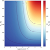 |
Fig. B.1 Excitation temperature of [O I] 63 μm for a combination of kinetic temperature and density of the gas. We have added contour levels for excitation temperatures of 20, 50, 100 and 150 K. |
The excitation temperature of a transition is related to the ratio of the level population through the Boltzmann equation by:
![Mathematical equation: $\[\frac{n_j}{n_i}=\frac{g_j}{g_i} \exp \left[-\left(E_j-E_i\right) / k_{\mathrm{b}} T_{\mathrm{ex} i j}\right],\]$](/articles/aa/full_html/2024/10/aa50530-24/aa50530-24-eq45.png) (B.5)
(B.5)
with g the statistical weight and E energy of a level. Upward and downward collision rates are related by:
![Mathematical equation: $\[C_{j i}=C_{i j} \frac{g_i}{g_j} \exp \left(-h \nu_{i j} / k_{\mathrm{b}} T_{\text {kin }}\right).\]$](/articles/aa/full_html/2024/10/aa50530-24/aa50530-24-eq46.png) (B.6)
(B.6)
Here, we selected molecular hydrogen as main collision partner with an orto-to-para ratio of 3:1. The resulting excitation temperatures for [O I] 63 μm and [O I] 145 μm as a function of kinetic temperature and density are shown in Fig. B.1 and B.2, respectively.
Using these dependencies we can obtain the [O I] 145 μm excitation temperature from the [O I] 63 μm excitation temperature if we assume either a particular gas density or kinetic temperature. We can simply look up the parameters in Fig. B.1 that produce the [O I] 63 μm excitation temperature measured in the first step and go with these parameters into Fig. B.2 to obtain the [O I] 145 μm excitation temperature. Here, we assumed a density of 106 cm−3, as an intermediate value given the critical density of both transitions. A different method would be to fix the kinetic temperature and then search for a density. The methods are equivalent and the actual choice of the method or the value are not significant when it comes to the final output. Actually, it is not necessary to have a precise value for the [O I] 145 μm excitation temperature because the quantity entering the radiative transfer is the emissivity (B(Tex) × τ145) – and not Tex as such. In Fig. B.3, we plot in colors the [O I] 145 μm emissivity (B(Tex) × τ145) as a function of the kinetic temperature and column density on a Rayleigh-Jeans scale. We can see that the [O I] 145 μm emissivity and the [O I] 63 μm excitation temperature go almost in parallel. Thus, if we have a given Tex,63, we can read the [O I] 145 μm emissivity with reasonable accuracy. We do not need to know the exact excitation temperature of the [O I] 145 μm line and the corresponding gas density and temperature. We see that for a Tex,63 of 75 K and below, the [O I] 145 μm emissivity stays almost constant along the contours, it is independent of the actual density. Hence, we have no significant uncertainty in the background column from the method. At higher Tex,63 we can conclude that we are still safe against variations towards higher densities, but that, for example, for Tex,63 = 100 K, we underestimate the emissivity by a factor 2 if the actual gas density is 105 cm−3 instead of 106 cm−3 so that we overestimate the background component column by this factor of two.
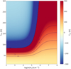 |
Fig. B.2 Excitation temperature of [O I] 145 μm for a combination of kinetic temperature and density of the gas. We have added contour levels for excitation temperatures of 100, 150, 200 and 250 K. |
Altogether, we have estimated the excitation temperature in a 3-step process: 1) selection of an excitation temperature from [O I] 63 μm main beam temperature peak, 2) estimation of the kinetic temperature of oxygen from Fig. B.1 under the assumption of a density of 106 cm−3, together with the excitation temperature from 1), 3) estimate of the excitation temperature for [O I] 145 μm from Fig. B.2. The derived excitation temperatures for both transitions and the kinetic ones are shown in Table 3.
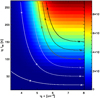 |
Fig. B.3 [O I] 145 μm emissivity in colors for a given column density. The contours are the [O I] 63 μm excitation temperature as in Fig. B.1. |
Appendix C Variation of parameters for background and foreground
C.1 Effects of varying the density of the background layer
In this subsection, we analyze the dependency of the derived physical parameters on the assumed value for the density of the background layer. As the default, we have considered a density of 106 cm−3 for deriving the upper transition excitation temperature from the lower transition excitation temperature, estimated from the peak brightness of the [O I] 63 μm line. Figure C.1 shows how changes in the assumed collision partner density of the background, and hence different values for the derived Tex,145 (derived from the analytic solution of the three-level system in Appendix B), result in different best-fit results for the background (dashed line) and foreground column density (solid line). We have selected two positions for each source to be analyzed in exploring the boundaries of our solutions. The other positions are affected in the same way.
The analysis shows that an increase in density leads to a corresponding increase in the estimated background column density and vice versa. This proportionality can be explained according to Fig. B.2, which illustrates the effect that the upper [O I] line shows a regime of population inversion. Any increase in density results in a decrease in the [O I] 145 μm excitation temperature (and vice versa) and, consequently, an increase in the [O I] column density necessary to maintain the observed intensity. In comparison, the [O I] 63 μm excitation temperature remains constant. Note that M17 SW position 4 can only be fitted with densities higher than 105 cm−3. For lower densities, the [O I] 145 μm peak intensity cannot be reached. It is worth noting that position 4 has the highest [O I] 145 μm intensity and is located at the [O I] peak, suggesting that the density here should be much higher than the other positions.
The foreground column density necessary for the deep absorption features depends very little on the background layer’s density variation, as is illustrated in Fig C.1. This insensibility is evident as the [O I] 63 μm absorption is highly optically thick so that the increase in the background intensity to be absorbed does not need to be compensated by an enhanced foreground absorption. The modest variations visible in the fit result originate in second-order effects. Depending on the details of the line profiles, the optically thinner wings of the absorbing layers are more or less sensitive to an increase or decrease in the background intensity resulting from the density variations.
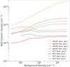 |
Fig. C.1 Best-fit column densities compared for selected positions against a range in the assumed density. The background is indicated by dashed lines and the foreground in solid ones. |
C.2 Effects of varying the kinetic temperature of the background layer
Now, let us continue analyzing the sensitivity of the derived background and foreground column densities against the second physical parameter, the kinetic temperature of the background, keeping the density fixed at 106cm−3. Above, we have assumed the kinetic temperature derived from the upward Rayleigh-Jeans corrected peak brightness temperature of the [O I] 63 μm emission shining through between the absorption dips, giving a lower limit to the excitation temperature. As the kinetic temperature is always larger than the excitation temperature (see Fig. B.2) for any density, this is also a lower limit to the kinetic temperature of the background. We now vary the kinetic temperature of the background from this minimum value up to higher values. We calculate the excitation temperatures for both [O I] lines from the analytic formulas at the given temperature and density (see Appendix B) and perform the least-squares fit of the line profiles with these parameters.
We stop increasing the kinetic temperature of the background once the background column density drops to the level of the foreground, breaking our initial assumption of having most of the material concentrated in the warm background layer. This upper limit gives the maximum kinetic temperature used in the fitting, roughly 50 K above our minimum value. Therefore, we have a reduced range of about 50 K for valid kinetic temperatures where our assumptions remain accurate.
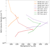 |
Fig. C.2 Best fit column densities compared for selected positions against a range in the assumed kinetic temperatures. |
Figure C.2 shows the thus fitted column densities for both layers against the range of background kinetic temperatures for selected positions fitted in Mon R2 and M17 SW. The figure shows that to fit the observed brightness of the background emission; the necessary background column density is roughly inversely proportional to the excitation temperature and, hence, the kinetic temperature.
The foreground column density is only slightly affected by the changes in the background. Increases in the background kinetic temperature lead to a rise in the background excitation and main beam temperatures, reducing the optical depth due to the severe reduction in column density. Then, the higher background intensity requires more foreground material to absorb the background emission and obtain the observed self-absorbed profile. In any case, the range of variation is lower than an order of magnitude, keeping the foreground density well-constrained.
C.3 Effect of variations in the foreground excitation temperature
We now analyze how changes in the foreground excitation temperature assumed for the [O I] 63 μm line affect the foreground column density. For the previous analysis, we have assumed a temperature of 20 K. Figure C.3 shows how the foreground column density derived from the line profile changes when the foreground’s excitation temperature varies. We varied the foreground excitation temperature from 15 K to 45 K and selected 15 K as a lower limit because this value is the lowest possible for [ C II] from the energy balance (Kabanovic et al. 2022), a reasonable assumption where both atoms should coexist. There is insufficient material to absorb the background in some positions for lower values than this, establishing a lower limit to the foreground excitation temperature. The upper value of 45 K is an appropriate upper limit for the foreground gas to produce visible absorption nodges still; higher values come too close to the background values.
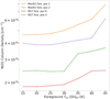 |
Fig. C.3 Best fit foreground column densities compared for selected positions against a range in the assumed foreground excitation temperatures. |
References
- Beckwith, S., Evans, N. J., I., Becklin, E. E., & Neugebauer, G. 1976, ApJ, 208, 390 [NASA ADS] [CrossRef] [Google Scholar]
- Bohlin, R. C., Savage, B. D., & Drake, J. F. 1978, ApJ, 224, 132 [Google Scholar]
- Boreiko, R. T., & Betz, A. L. 1996, ApJ, 464, L83 [NASA ADS] [CrossRef] [Google Scholar]
- Colditz, S., Beckmann, S., Bryant, A., et al. 2018, J. Astron. Instrum., 7, 1840004 [Google Scholar]
- Fernández-Ontiveros, J. A., Spinoglio, L., Pereira-Santaella, M., et al. 2016, ApJS, 226, 19 [CrossRef] [Google Scholar]
- Fischer, C., Beckmann, S., Bryant, A., et al. 2018, J. Astron. Instrum., 7, 1840003 [Google Scholar]
- Ginard, D., González-García, M., Fuente, A., et al. 2012, A&A, 543, A27 [NASA ADS] [CrossRef] [EDP Sciences] [Google Scholar]
- Goldsmith, P. F. 2019, ApJ, 887, 54 [NASA ADS] [CrossRef] [Google Scholar]
- Goldsmith, P. F., Yıldız, U. A., Langer, W. D., & Pineda, J. L. 2015, ApJ, 814, 133 [Google Scholar]
- Goldsmith, P. F., Langer, W. D., Seo, Y., et al. 2021, ApJ, 916, 6 [NASA ADS] [CrossRef] [Google Scholar]
- Goldsmith, P. F., Langer, W. D., Seo, Y., et al. 2023, ApJ, 952, 102 [NASA ADS] [CrossRef] [Google Scholar]
- González-Alfonso, E., Fischer, J., Graciá-Carpio, J., et al. 2012, A&A, 541, A4 [NASA ADS] [CrossRef] [EDP Sciences] [Google Scholar]
- Griffin, M. J., Abergel, A., Abreu, A., et al. 2010, A&A, 518, L3 [EDP Sciences] [Google Scholar]
- Guan, X., Stutzki, J., Graf, U. U., et al. 2012, A&A, 542, L4 [NASA ADS] [CrossRef] [EDP Sciences] [Google Scholar]
- Guevara, C., Stutzki, J., Ossenkopf-Okada, V., et al. 2020, A&A, 636, A16 [CrossRef] [EDP Sciences] [Google Scholar]
- Gusdorf, A., Anderl, S., Lefloch, B., et al. 2017, A&A, 602, A8 [NASA ADS] [CrossRef] [EDP Sciences] [Google Scholar]
- Harris, A. I., Stutzki, J., Genzel, R., et al. 1987, ApJ, 322, L49 [NASA ADS] [CrossRef] [Google Scholar]
- Heyminck, S., Graf, U. U., Güsten, R., et al. 2012, A&A, 542, L1 [NASA ADS] [CrossRef] [EDP Sciences] [Google Scholar]
- Hoffmeister, V. H., Chini, R., Scheyda, C. M., et al. 2008, ApJ, 686, 310 [NASA ADS] [CrossRef] [Google Scholar]
- Hollenbach, D. J., & Tielens, A. G. G. M. 1999, Rev. Mod. Phys., 71, 173 [Google Scholar]
- Kabanovic, S., Schneider, N., Ossenkopf-Okada, V., et al. 2022, A&A, 659, A36 [NASA ADS] [CrossRef] [EDP Sciences] [Google Scholar]
- Kirsanova, M. S., Ossenkopf-Okada, V., Anderson, L. D., et al. 2020, MNRAS, 497, 2651 [NASA ADS] [CrossRef] [Google Scholar]
- Klein, R., Reedy, A., Fischer, C., et al. 2023, ApJ, 945, 29 [NASA ADS] [CrossRef] [Google Scholar]
- Kristensen, L. E., Gusdorf, A., Mottram, J. C., et al. 2017, A&A, 601, L4 [NASA ADS] [CrossRef] [EDP Sciences] [Google Scholar]
- Le Petit, F., Nehmé, C., Le Bourlot, J., & Roueff, E. 2006, ApJS, 164, 506 [NASA ADS] [CrossRef] [Google Scholar]
- Leurini, S., Wyrowski, F., Wiesemeyer, H., et al. 2015, A&A, 584, A70 [NASA ADS] [CrossRef] [EDP Sciences] [Google Scholar]
- Lique, F., Klos, J., Alexander, M. H., Le Picard, S. D., & Dagdigian, P. J. 2018, MNRAS, 474, 2313 [NASA ADS] [CrossRef] [Google Scholar]
- Meixner, M., Haas, M. R., Tielens, A. G. G. M., Erickson, E. F., & Werner, M. 1992, ApJ, 390, 499 [NASA ADS] [CrossRef] [Google Scholar]
- Mookerjea, B., Sandell, G., Güsten, R., et al. 2019, A&A, 626, A131 [NASA ADS] [CrossRef] [EDP Sciences] [Google Scholar]
- Palmeirim, P., André, P., Kirk, J., et al. 2013, A&A, 550, A38 [NASA ADS] [CrossRef] [EDP Sciences] [Google Scholar]
- Pérez-Beaupuits, J. P., Güsten, R., Spaans, M., et al. 2015a, A&A, 583, A107 [NASA ADS] [CrossRef] [EDP Sciences] [Google Scholar]
- Pérez-Beaupuits, J. P., Stutzki, J., Ossenkopf, V., et al. 2015b, A&A, 575, A9 [NASA ADS] [CrossRef] [EDP Sciences] [Google Scholar]
- Pilleri, P., Fuente, A., Cernicharo, J., et al. 2012, A&A, 544, A110 [NASA ADS] [CrossRef] [EDP Sciences] [Google Scholar]
- Pilleri, P., Treviño-Morales, S., Fuente, A., et al. 2013, A&A, 554, A87 [NASA ADS] [CrossRef] [EDP Sciences] [Google Scholar]
- Rayner, T. S. M., Griffin, M. J., Schneider, N., et al. 2017, A&A, 607, A22 [NASA ADS] [CrossRef] [EDP Sciences] [Google Scholar]
- Risacher, C., Güsten, R., Stutzki, J., et al. 2016, A&A, 595, A34 [NASA ADS] [CrossRef] [EDP Sciences] [Google Scholar]
- Schneider, N., Röllig, M., Simon, R., et al. 2018, A&A, 617, A45 [NASA ADS] [CrossRef] [EDP Sciences] [Google Scholar]
- Schneider, N., Simon, R., Guevara, C., et al. 2020, PASP, 132, 104301 [NASA ADS] [CrossRef] [Google Scholar]
- Stacey, G. J., Smyers, S. D., Kurtz, N. T., & Harwit, M. 1983, ApJ, 265, L7 [NASA ADS] [CrossRef] [Google Scholar]
- Stutzki, J., Stacey, G. J., Genzel, R., et al. 1988, ApJ, 332, 379 [NASA ADS] [CrossRef] [Google Scholar]
- Temi, P., Hoffman, D., Ennico, K., & Le, J. 2018, J. Astron. Instrum., 7, 1840011 [NASA ADS] [CrossRef] [Google Scholar]
- Tielens, A. G. G. M., & Hollenbach, D. 1985, ApJ, 291, 722 [Google Scholar]
- Treviño-Morales, S. P., Pilleri, P., Fuente, A., et al. 2014, A&A, 569, A19 [NASA ADS] [CrossRef] [EDP Sciences] [Google Scholar]
- Treviño-Morales, S. P., Fuente, A., Sánchez-Monge, Á., et al. 2019, A&A, 629, A81 [NASA ADS] [CrossRef] [EDP Sciences] [Google Scholar]
- Wakelam, V., & Herbst, E. 2008, ApJ, 680, 371 [NASA ADS] [CrossRef] [Google Scholar]
- Wiese, W. L., & Fuhr, J. R. 2007, J. Phys. Chem. Ref. Data, 36, 1287 [CrossRef] [Google Scholar]
- Wu, Y. W., Reid, M. J., Sakai, N., et al. 2019, ApJ, 874, 94 [NASA ADS] [CrossRef] [Google Scholar]
- Young, E. T., Becklin, E. E., Marcum, P. M., et al. 2012, ApJ, 749, L17 [NASA ADS] [CrossRef] [Google Scholar]
- Zucker, C., Speagle, J. S., Schlafly, E. F., et al. 2019, ApJ, 879, 125 [NASA ADS] [CrossRef] [Google Scholar]
upGREAT is a development by the MPI für Radioastronomie and KOSMA/Universität zu Köln, in cooperation with the DLR Institut für Optische Sensorsysteme.
For details on the observing scheme, see Schneider et al. (2020).
All Tables
Mon R2 and M17 SW background excitation temperatures for both transitions and their respective kinetic temperatures.
Mon R2 and M17 SW [O I] 145 μm and [O I] 63 μm background column density per position for the two layer model.
Mon R2 and M17 SW [O I] 63 μm foreground column density per position for the two-layer model.
Mon R2 and M17 SW comparison between oxygen and ionized carbon column densities and equivalent extinctions for the background columns.
Mon R2 and M17 SW comparison between oxygen and ionized carbon column densities and equivalent extinctions for the foreground columns.
All Figures
|
Fig. 1 Mon R2 [C II] integrated intensity map for the velocity range between 0 and 30 km s−1 with the two [C II] single pointings (in black) from Guevara et al. (2020). [O I] 63 μm integrated intensity map in blue contours covering the same velocity range of [C II] (levels at 100, 150, 200, 240, 270, and 300 K km s−1). The white circle represents the FWHM beam size of both maps, 15″. |
| In the text | |
|
Fig. 2 M17 SW [C II] integrated intensity map for the velocity range between 0 and 40 km s−1 with the original [C II] single pointings (in black) from Guevara et al. (2020) (equivalent to a LFA array pointing). [O I] 63 μm integrated intensity map in blue contours covering the same velocity range of [C II] (levels at 40, 70, 100, 120, 140, and 160 and 200 K km s−1). The black circle shows the FWHM beam size for both maps, 15″. |
| In the text | |
|
Fig. 3 Mon R2 [O I] 63 μm, [O I] 145 μm, [12C II] and [13C II] spectra for the single pointings previously observed in [C II]. All spectra have been convolved to a beam size of 15″. The vertical dashed lines at the 8 and 11 km s−1 absorption dip are present in both spectra, below the horizontal dashed line at 0 K. The [13C II] has been smoothed in velocity for a matter of display. |
| In the text | |
|
Fig. 4 Mon R2 [O I] 63 μm, [O I] 145 μm, and [C II] mosaic spectra for the central area of the source. The dotted lines are located at 5, 10, 15, and 20 km s−1, respectively. The angular resolution is the same for [C II], [O I] 145 μm and [O I] 63 μm (15″), with a grid spacing of 10″. The offset coordinates of each spectrum with respect to the source position are given in the top-left corner of each box. |
| In the text | |
|
Fig. 5 Same as Fig. 3, but for M17 SW. The dotted lines mark the two absorption dips present for both fine structure lines at 21 and 24 km s−1. |
| In the text | |
|
Fig. 6 M17 SW [O I] 63 μm, [O I] 145 μm, and [C II] mosaic. The two dotted vertical lines per spectrum are located at 22 and 24 km s−1, respectively, added to guide the eye to the absorption dips. The upper left corner in each box gives the offsets of each spectrum. |
| In the text | |
|
Fig. 7 Mon R2 [O I] fits for position 2 for both transitions. The background fit needs 7 components, the 2 coming from the [O I] 145 μm line carrying the bulk of the column density, plus 5 additional weak ones. The foreground fit needs 6 components. Top: Mon R2 [O I] 145 μm fitting for position 2. Top left: This panel represents the fitted model in blue and the observed spectra in red. Bottom left: residual curve between the observed spectra and the model. Right: composition of each fitted component in cyan. Bottom: Mon R2 [O I] 63 μm fitting for position 2. Top left: fitted model in blue and the observed spectra in red. Bottom left: residual curve between the observed spectra and the model. Top right: composition of each fitted component in cyan and the fitted [O I] 63 μm background profile in orange. Bottom right: foreground optical depth for the [O I] 63 μm line of each Gaussian component in pink. |
| In the text | |
|
Fig. 8 Compilation of background Gaussian parameters for all positions from the multi-component analysis from Sec. 3. Each position is plotted in columns along the velocity axis, showing both atomic lines. Circles symbolize the [O I] Gaussian components for each position and triangles the [ C II] ones (from Guevara et al. 2020). The color of each symbol represents its column density. The length of the vertical bars denotes half of the line width value for a better visualization. |
| In the text | |
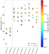 |
Fig. 9 Same as Fig. 8 for the foreground parameters. |
| In the text | |
|
Fig. 10 Unsuccessful (note the significantly increased level of the residuals) fit for M17 SW pos. 6, using the foreground parameters fitted to position 0. |
| In the text | |
|
Fig. 11 Same as Fig. 10, using the foreground parameters fitted to position 0, but allowing for variations in width and column density. |
| In the text | |
|
Fig. B.1 Excitation temperature of [O I] 63 μm for a combination of kinetic temperature and density of the gas. We have added contour levels for excitation temperatures of 20, 50, 100 and 150 K. |
| In the text | |
|
Fig. B.2 Excitation temperature of [O I] 145 μm for a combination of kinetic temperature and density of the gas. We have added contour levels for excitation temperatures of 100, 150, 200 and 250 K. |
| In the text | |
|
Fig. B.3 [O I] 145 μm emissivity in colors for a given column density. The contours are the [O I] 63 μm excitation temperature as in Fig. B.1. |
| In the text | |
|
Fig. C.1 Best-fit column densities compared for selected positions against a range in the assumed density. The background is indicated by dashed lines and the foreground in solid ones. |
| In the text | |
|
Fig. C.2 Best fit column densities compared for selected positions against a range in the assumed kinetic temperatures. |
| In the text | |
|
Fig. C.3 Best fit foreground column densities compared for selected positions against a range in the assumed foreground excitation temperatures. |
| In the text | |
Current usage metrics show cumulative count of Article Views (full-text article views including HTML views, PDF and ePub downloads, according to the available data) and Abstracts Views on Vision4Press platform.
Data correspond to usage on the plateform after 2015. The current usage metrics is available 48-96 hours after online publication and is updated daily on week days.
Initial download of the metrics may take a while.