© The Authors 2024

1. Introduction

The missing mass problem has not yet been fully resolved. The usual solution is to assume the validity of Newtonian dynamics and general relativity and to postulate the existence of dark matter (DM) (see, e.g., Salucci 2019 for a review). While many types of dark matter have been proposed, for concreteness, we focus on the cold dark matter (CDM) and the Lambda cold dark matter (ΛCDM) cosmological model in the present work. In the ΛCDM model, many well-known observations, particularly on the cosmological scales, can be explained well (cosmic microwave background, baryon acoustic oscillations, distance-luminosity relation for type II supernovae, etc.). However, many questions remain unexplained, such as the mismatch between the Hubble constant in the early and late Universe (Verde et al. 2019), large-scale cosmic flows (Peery et al. 2018), emptiness of the Local Void (Peebles & Nusser 2010; Haslbauer et al. 2020), and existence of the planes of satellites (Pawlowski et al. 2019), among others. The internal properties of galaxies cannot be predicted in full from the first principles and they are even hard to reproduce in simulations (Brooks & Christensen 2016; Oman et al. 2015; Bullock & Boylan-Kolchin 2017), while simple, tight scaling relations between the baryonic and DM content have indeed been observed (Persic et al. 1996; Famaey & McGaugh 2012; McGaugh et al. 2016).

Another option is to explain the missing mass problem without DM particles outside of the standard models of particle physics. This is the case of modified Newtonian dynamics (MOND) (Milgrom 1983) paradigm, according to which our knowledge of the law of gravity and/or inertia should be corrected in the limit of small accelerations (see, e.g., reviews Milgrom 2015b, 2014b; Famaey & McGaugh 2012). Hereafter, we consider only the MOND modified gravity theories. Although MOND was initially devised on the basis of the first rough observations of rotation curves, it provides formulas that allow for the dynamics of a wide range of galaxies to be predicted, where the most reliable measurements also show the best agreement (Lelli et al. 2017; Li et al. 2018). Importantly, for the present paper, MOND also has been tested successfully on the scale of hundreds and thousands of kpc via weak gravitational lensing (Milgrom 2013; Mistele et al. 2024a,b) and the dynamics of galaxy groups (Milgrom 2018, 2019). The open questions for MOND include the nature of the remaining missing mass problem of galaxy clusters (Milgrom & Sanders 2008), the survivability and dynamics of ultra-diffuse galaxies in these environments (Milgrom 2015a; Freundlich et al. 2022), the internal dynamics of globular clusters (Ibata et al. 2013; Hernandez & Lara-DI 2020), and, finally, establishing a covariant version of MOND that would simultaneously explain all the available data (Famaey & McGaugh 2012; Mistele et al. 2023). While MOND might not be the definitive solution to the missing mass problem, the above results show that if a modified gravity theory is governing our Universe, then MOND must be its excellent approximation on the scale of galaxies and galaxy groups.

A key aspect of MOND (and absent w.r.t. Newtonian gravity) is external field effect (EFE). It is a manifestation of the non-linearity of MOND theories; namely, in MOND, the superposition principle for gravitational fields does not hold true (Milgrom 2014a). In reality, galaxies are always embedded in some external field that is generated by nearby galaxies, galaxy clusters and large-scale cosmological structures. The external field is, of course, different for each object, but has been estimated to be typically on the order of a few percent of a₀ (Famaey et al. 2007; Wu et al. 2008; Hees et al. 2016; Milgrom 2018; Oria et al. 2021); however, it can be much higher, for example, for satellites of galaxies or for galaxies in clusters (Müller et al. 2019; Freundlich et al. 2022).

In modified gravity theories that do not involve DM, we introduce the concept of “phantom dark matter” (PDM, Milgrom 1986). It is a mathematical construct that denotes the dark matter that would lead in the Newtonian gravity to the observed gravitational field while actually a modified gravity theory holds true. The distribution of PDM can be very unusual or even impossible from the point of view of the Newtonian gravity. For example, in MOND, the PDM around a point mass has a zero density in the vicinity of the point, but at larger radii it mimics an isothermal halo. This is in stark contrast to the Navarro-Frenk-White DM halo expected by the theory of ΛCDM, which has an infinite density in its center (Navarro et al. 1996). For some configurations of baryonic matter, the density of PDM can even be negative in some regions of space. Milgrom (1986) identified a few specific mass configurations that give rise to negative density of PDM: a pair of point masses, a disk with a hole in its center, an inhomogeneous thin galactic disk, and an infinitesimal mass embedded in a homogeneous external gravitational field. Oria et al. (2021) made maps of the regions of the negative PDM for the Local Volume. The distribution of PDM around an object depends, in general, on the external field imposed on it by other objects. Also, it can strongly depend on the particular MOND theory (Milgrom 2023).

To distinguish modified gravity from DM by the EFE (Milgrom 1983), various astrophysical tests have been proposed, based on either dynamical friction (Kroupa 2015), the dynamics of wide binary stars (Hernandez et al. 2012), and others; however, all these tests have their respective disadvantages. Another way to distinguish between various solutions to the missing mass problem would be to inspect the halos (real or phantom) of galaxies, their groups and clusters by weak gravitational lensing. All these objects are expected to have virialized DM halos in the theories involving particle DM. Their detailed profiles depend on the type of the DM particle. However, they cannot replicate the shapes of all PDM halos, such as those with negative densities.

In all relativistic MOND theories known thus far, calculating gravitational lensing is not particularly difficult: we can apply the procedures known from general relativity on the sum of the densities of baryonic matter and of the PDM (Milgrom 2013). This has been used to explain some observations. For example, Jee et al. (2007) reported the discovery of a ring of DM around the galaxy cluster Cl 0024+17. Milgrom & Sanders (2008) showed that such rings are expected to be detected if MOND works, but Newtonian gravity is assumed for the reconstruction of the surface density map, since sufficiently compact objects generate PDM halos with central cavities. Establishing whether such rings of DM are common will be a strong test of MOND. Milgrom (2013) showed that the observed halos of galaxies follow MOND predictions. There were even hints that the measured dark halos are cut off at about 200 kpc. In MOND, this is explained (as detailed in Sect. 6) by the external field effect. Mistele et al. (2024a) demonstrated that for very isolated galaxies, the lensing agrees with MOND predictions up to very large galactocentric distances. Strong lensing in MOND is not expected to deviate much from Newtonian gravity without DM (Sanders & Land 2008; Tian & Ko 2017; Milgrom 2020).

In the current paper, we investigate PDM halos of point masses and their pairs and the influence of the EFE on them in detail. We also present the predicted maps of gravitational lensing around them; in particular for the QUMOND modified gravity version of MOND (Milgrom 2010). The point masses are assumed to represent galaxies, galaxy groups, and clusters as a zeroth order approximation. We investigate whether the special effects of MOND distinguishing it from the ΛCDM cosmology are within reach of the current instruments. The topic is particularly timely since the recently launched Euclid satellite is expected to revolutionize the field of weak lensing. It will survey about 1/3 of the sky with an angular resolution comparable to the Hubble Space Telescope. The multitude of the photometric filters will not only enable us to determine the redshifts of the lensed galaxies, but the accurate stellar masses of the lenses as well, which are needed for predicting the gravitational field in MOND. Unlike the distinguishing test of MOND and particle DM based on dynamical measurements, weak lensing does not impose any assumptions on the dynamics of the investigated objects (such as being in virial equilibrium) and is insensitive to many of the uncertain aspects of galaxy evolution.

The paper is organized as follows. We explain how to calculate the PDM density in QUMOND in Sect. 2. Then we recall the weak lensing formalism in general in Sect. 3. We progress to the case of a single point mass in Sect. 6. We discuss the case where there is no external field (Sect. 6.1), external field with a known direction (Sect. 6.2) and external field with an unknown direction (Sect. 6.3). We also compare the QUMOND predicted PDM halo to a dark halo in the ΛCDM cosmology in Sect. 6.4. Section 7 is devoted to a pair of point masses, observed either perpendicularly to the connecting line (Sect. 7.2) or along it (Sect. 7.3). The external field is treated in an approximate way and, therefore, this approximation is justified in detail in Sect. 7.4. In Sect. 8, we estimate whether the deviation of QUMOND from Newtonian gravity can be achieved with the current instruments and we find that it indeed appears to be feasible. We summarize our findings in Sect. 9. In this paper, the symbol f() denotes an unspecified function of the parameters in parentheses. The natural logarithm is denoted as ln, while the decadic logarithm as log₁₀.

2. Calculating the effective distribution of the lensing mass in modified gravity

We base the present work on the QUMOND theory, since it provides an especially simple way to calculate the density of PDM ρ_ph, namely, as:

$$\begin{array}{c}\hfill {\rho }_{\mathrm{ph}}=\frac{-1}{4\pi G}\mathrm{\nabla }\left[\nu \left(\frac{g_N}{a_0}\right){\mathbf{g}}_N\right],\end{array}$$(1)

where g_N stands for the gravitational acceleration calculated in the usual Newtonian way from the distribution of the baryonic matter, a₀ stands for the acceleration constant of the MOND theory, a₀ ≈ 1.2 × 10⁻¹⁰ m s⁻² (McGaugh 2011; McGaugh et al. 2016; Lelli et al. 2017), and ν for the interpolating function. The theory does not give a concrete prescription for ν, but it dictates its behavior in two limits: (1) ν(x)≈1 for x ≫ 1, such that the Newtonian gravity is restored for high accelerations and (2) ν(x)≈x^−1/2 for x ≪ 1, such that flat rotation curves of galaxies are reproduced at small accelerations. In this paper, we assume the observationally motivated ν function as:

$$\begin{array}{c}\hfill \nu (x)=\frac{1}{1-e^{-\sqrt{x}}},\end{array}$$(2)

which can explain the rotation of H I gas clouds in galaxies excellently (McGaugh et al. 2016; Li et al. 2018). In this paper, we are interested in gravitational lensing around a point mass or a pair of point masses. For these simple mass configurations, we were able to obtain analytic expressions for the density of PDM effectively. For a more complex distribution of sources, public codes do exist to evaluate the density distribution of PDM numerically (Lüghausen et al. 2015; Candlish et al. 2015).

In Appendix A, we derive general functional forms for the density and surface density of the PDM in the deep-MOND regime of any MOND theory, whereby the concept of PDM makes sense and does not introduce any other new constants of physics than a₀. That is to say, if M denotes the total baryonic mass of the system, d its characteristic size, g_e the magnitude of the external field, and α a vector of dimensionless parameters that describe the geometry of the problem, then:

$$\begin{array}{c}\hfill {\rho }_{\mathrm{ph}}(\mathit{x})=\frac{1}{d^2}\sqrt{\frac{M{a}_0}{G}}f(\mathit{\alpha },\frac{\mathit{x}}{d},\frac{g_{e}d}{\sqrt{GM{a}_0}})-{\rho }_{\mathrm{b}}(\mathit{x}),\end{array}$$(3)

and

$$\begin{array}{c}\hfill {\mathrm{\Sigma }}_{\mathrm{ph}}(\mathit{\xi })=\frac{1}{d}\sqrt{\frac{M{a}_0}{G}}f(\mathit{\alpha },\frac{\mathit{\xi }}{d},\frac{g_{e}d}{\sqrt{GM{a}_0}})-{\mathrm{\Sigma }}_{\mathrm{b}}(\mathit{\xi }),\end{array}$$(4)

where ρ_b and Σ_b denote the density and surface density of the baryonic matter, respectively.

3. Methods to predict the maps of gravitational lensing

In this section, we review the basics of gravitational lensing. We follow Bartelmann & Maturi (2017) with some details complemented from Bartelmann & Schneider (2001). When the light emitted by a distant source (typically a galaxy) passes around a massive object called the lens, located between the source and the observer, its path is bent. As a result, the observer captures a deformed image of the source. In the weak lensing limit, that is when the deformations are small, the transformation of the image can be considered linear, such that the images of circular sources are ellipses. Such a linear mapping can be understood as a combination of flattening, rotation, magnification, and shift of the original image. If the linear approximation is not sufficient, we are then dealing with strong lensing. As was shown for spherically symmetric lenses, MOND predicts only a small deviation from the Newtonian gravity without DM in the strong-lensing regime (Milgrom 2012). This prediction agrees with observations (Tian & Ko 2017). Later in this paper we confirm that MOND does not give rise to strong lensing in its weak-field regime even for lenses without the circular symmetry.

Most observational characteristics of gravitational lensing can be derived from the lensing potential, ψ. If the thickness of the mass distribution of the lens is negligible compared to the distances to of the lens from the source and from the observer, which is the case of the astrophysical situations of interest of this paper, then we can make the so-called thin lens approximation. Thus, the lensing potential can be calculated as

$$\begin{array}{c}\hfill \mathrm{\Delta }\psi (\mathit{\theta })=2\frac{\mathrm{\Sigma }(\mathit{\theta })}{{\mathrm{\Sigma }}_{\mathrm{cr}}},\end{array}$$(5)

where

$$\begin{array}{c}\hfill \mathrm{\Sigma }(\mathit{\theta })={\displaystyle {\int }_{-\infty }^{\infty }}\rho (\mathit{\theta },z)\mathrm{d}z,\end{array}$$(6)

and

$$\begin{array}{c}\hfill {\mathrm{\Sigma }}_{\mathrm{cr}}^{-1}=\frac{4\pi G}{c^2}\frac{D_L{D}_{\mathit{LS}}}{D_S}.\end{array}$$(7)

In these formulas, $\mathit{\theta }=({\theta }_1,{\theta }_2)$ is a vector, expressed in the units of radians, in a Cartesian system that touches the celestial sphere at the position of the lens from the point of view of the observer. For circularly symmetric lenses, we match the origin of the coordinate system with the center of the symmetry. The symbol Δ stands for the two-dimensional (2D) Laplace operator with respect to the coordinates θ. The surface density Σ in Eq. (6) is given by integration of the volume density, ρ, of the lens along the line of sight, z. In the context of this paper, ρ is the sum of the density of the baryonic matter and the PDM. The constant Σ_cr is called the critical surface density. In Eq. (7), D_L denotes the angular-diameter distance of the lens from the observer, D_S the angular-diameter distance of the source from the observer, and D_LS the angular-diameter distance of the source for an observer at the lens at the cosmic time when the photon passes the lens. For a point mass, M, (without a PDM halo) we have

$$\begin{array}{c}\hfill \psi (\mathit{\theta })=\frac{4GM}{c^2}\frac{D_{\mathit{LS}}}{D_L{D}_S}ln\theta .\end{array}$$(8)

The Jacobian matrix characterizes locally the deformation of the image by the lens. It is defined as

$$\begin{array}{c}\hfill A_{\mathit{ij}}(\mathit{\theta })={\delta }_{\mathit{ij}}-\frac{{\partial }^2\psi (\mathit{\theta })}{\partial {\theta }_i\partial {\theta }_j},\end{array}$$(9)

where δ_ij is Kronecker’s symbol. If we calculate the eigenvectors, e₊ and e₋, and the corresponding eigenvalues, λ₊ and λ₋, of the inverse of the Jacobian matrix, A⁻¹, we learn to what sort of ellipse a circular source is deformed into. The major axis of the ellipse points in the direction of e₊ that corresponds to the larger eigenvalue λ₊. The ratio of the eigenvalues is equal to the ratio of the axes of the ellipse. The complex ellipticity (one of the two common definitions that is related more directly to observations, see Bartelmann & Schneider 2001) is defined as

$$\begin{array}{c}\hfill ϵ=\frac{{\lambda }_{+}-{\lambda }_{-}}{{\lambda }_{+}+{\lambda }_{-}}{e}^{2\varphi i},\end{array}$$(10)

where ϕ denotes the position angle of the major axis of the ellipse. We can also express ϵ as a sum of its real and imaginary part, ϵ = ϵ₁ + iϵ₂. We use ellipticity here (without the complement of “complex”) to denote the magnitude of the complex ellipticity.

We define the shear as

$$\begin{array}{c}\hfill \gamma ={\gamma }_1+i{\gamma }_2,\end{array}$$(11)

where

$$\begin{array}{c}\hfill {\gamma }_1=\frac{1}{2}(\frac{{\partial }^2\psi }{\partial {\theta }_1^2}-\frac{{\partial }^2\psi }{\partial {\theta }_2^2}),{\gamma }_2=\frac{{\partial }^2\psi }{\partial {\theta }_1\partial {\theta }_2}.\end{array}$$(12)

In the case of small deformations of the image, namely, in the weak-lensing limit,

$$\begin{array}{c}\hfill ϵ\approx \gamma .\end{array}$$(13)

In the lowest order of approximation, the intrinsic complex ellipticity of the background source, ϵ_S, and the complex ellipticity caused by lensing add up, such that the total observed ellipticity of the source is ϵ_S + ϵ. This fact, along with the linearity of Eqs. (5) and (12), ensures that the surface density obtained by stacking of many lenses is the average of the surface densities of the individual lenses.

If the surface density of the lens is circularly symmetric, a simpler way of calculating the image deformation exists. The lens then deforms the image of the source only be stretching or squeezing along circles centered on the lens. We thus introduce the tangential shear as

$$\begin{array}{c}\hfill {\gamma }_t=-cos(2\varphi ){\gamma }_1-sin(2\varphi ){\gamma }_2.\end{array}$$(14)

It satisfies |ϵ|≈|γ_t| in the weak-lensing limit. Let us denote, using R, the projected radius form the center of the lens (in kpc), M(R) is then the projected mass contained within the radius, R, ϑ = R/D_L, and m(ϑ) = M(ϑD_L)/(πD_L²Σ_cr). Then

$$\begin{array}{c}\hfill {\gamma }_t(\vartheta )=\frac{m(\vartheta )}{{\vartheta }^2}-\frac{1}{2\vartheta }\frac{\mathrm{d}m(\vartheta )}{\mathrm{d}\vartheta }.\end{array}$$(15)

Next, the effects of gravitational lensing can be characterized by magnification. If we define the convergence

$$\begin{array}{c}\hfill \kappa =\mathrm{\Sigma }/{\mathrm{\Sigma }}_{\mathrm{crit}},\end{array}$$(16)

then magnification

$$\begin{array}{c}\hfill \mu \approx 1+2\kappa .\end{array}$$(17)

For axially symmetric lenses observed along the symmetry axes we have

$$\begin{array}{c}\hfill \kappa =-\frac{1}{2\vartheta }\frac{\mathrm{d}m(\vartheta )}{\mathrm{d}\vartheta }.\end{array}$$(18)

However, for the reconstruction of the density field, the magnification is not as useful as the shear; thus, here we focus on the shear.

4. Scaling with distance

Suppose that we have already calculated the lensing potential and shear for some distance of the lens, D_L, 0, source, D_S, 0 and their mutual distance, D_LS, 0. It would be useful to know how these results will change if the same lens is at D_L = aD_L, 0, and the source at D_S = bD_S, 0. Because angular diameter distances do not add up linearly, the distance between the lens and source will change to D_LS = cD_LS, 0, where c depends on D_L and D_S. From Eq. (8) and the linearity of Eq. (5), we obtain that the new lensing potential $\psi (\theta )=\frac{c}{\mathit{ab}}{\psi }_0(a\theta )$, where ψ₀ is function prescribing the original lensing potential. From here and Eq. (12) we get that the new shear γ is related to the original shear γ₀ as $\gamma (\theta )=\frac{\mathit{ac}}{b}{\gamma }_0(a\theta )$. Therefore, only the lensing ellipticity changes, not the positional angle.

5. Distances of the lenses and sources in the considered models

In all models considered in this paper, the lens is assumed to lie at the distance of D_L = 200 Mpc and the sources “in infinity”. We opted for this value for D_L because it is a rather typical value for the largest existing catalog of isolated galaxy pairs (Nottale & Chamaraux 2018) and the lensing by such objects is the primary objective of this paper. The future catalogs of isolated galaxy pairs will probably consist of relatively nearby galaxies too, because the measurements of radial velocities are necessary. At the distance of D_L = 200 Mpc, one arcsecond almost exactly corresponds to one kiloparsec.

We checked that the ratio D_LS/D_S appearing in Eq. (7) deviates from unity by less than four percent for redshifts higher than two and by less than six percent for redshifts higher than one. The numbers assume the final Planck cosmology (Planck Collaboration XVI 2014). For the purpose of this exploratory paper, we assume D_LS/D_S = 1. The shear published here can be rescaled to other distances of the sources by multiplying by the corresponding ratio D_LS/D_S.

6. Gravitational lensing by a point mass in QUMOND

6.1. Zero external field

Let us review the case of point mass that is in a zero external field. Gravitational acceleration g of any spherically symmetric object in QUMOND can be calculated as (Milgrom 2010):

$$\begin{array}{c}\hfill \mathit{g}={\mathit{g}}_{\mathit{N}}\nu (g_N/a_0).\end{array}$$(19)

By applying the Poisson equation to this field, one gets the density of the PDM. From Eq. (19), one can see that g ≈ g_N in the region where g_N ≫ a₀, that is well below the so-called MOND transitional radius

$$\begin{array}{c}\hfill r_{\mathrm{M}}=\sqrt{\frac{\mathit{GM}}{a_0}}.\end{array}$$(20)

Therefore, in the vicinity of the point mass the PDM halo nearly has a zero density if the interpolation function reaches one sufficiently rapidly for large arguments (Milgrom & Sanders 2008). This is the case of the interpolation function Eq. (2) assumed here. Well beyond the transitional radius, $g\approx \sqrt{g_N{a}_0}$. Then, for an isolated point mass, we obtain that the PDM density is equivalent to that of an isothermal sphere (e.g., Milgrom 2013)

$$\begin{array}{c}\hfill {\rho }_{\mathrm{IS}}=\frac{1}{4\pi r^2}\sqrt{\frac{M{a}_0}{G}},\end{array}$$(21)

which has the surface density of

$$\begin{array}{c}\hfill {\mathrm{\Sigma }}_{\mathrm{IS}}=\frac{1}{4r}\sqrt{\frac{M{a}_0}{G}}.\end{array}$$(22)

Milgrom & Sanders (2008) explored the surface distribution of PDM for a variety of circularly symmetric sources and interpolation functions. They found that MOND predicts rings in the surface density of PDM, unless the interpolation function reaches the high-acceleration limit too slowly. The maximum surface density of the ring is on the order of the constant Σ₀ = a₀/G = 8.6 × 10¹⁴ M_⊙ Mpc⁻² and it is reached approximately at the distance of r_M.

6.2. Known direction of the external field

Each object in the real Universe is however embedded in a nonzero external gravitation field that comes from the neighboring galaxies or the large-scale structures (Sect. 1). The external field is expected to affect the PDM halos at galactocentric distances larger than about the radius,

$$\begin{array}{c}\hfill r_{\mathrm{ef}}=\frac{\sqrt{GM{a}_0}}{g_e},\end{array}$$(23)

where the gravitational acceleration generated by the point mass $\sqrt{GM{a}_0}/r$ equals the external gravitational acceleration g_e (Milgrom 1983, 2014a). In our exploration of the PDM density distribution for a point mass in an homogeneous external field, we made use of Eq. (1). We assumed that the point mass is in the centre of a Cartesian coordinate system and the external gravitational field points in the direction of the positive z-axis. The resulting expression for the PDM density is stated in Appendix C. In Fig. 1, we plotted this density distribution for a point mass M = 10¹¹ M_⊙ and an external field g_e = 0.02 a₀. The dotted half-circle shows the radius, r_ef. One can note from here that the PDM halo is approximately spherical only below r_ef, where the external gravitational field is negligible compared to the field from the point mass. The central depression of the density of PDM is not visible in this figure because its size is just about 0.01 Mpc. Beyond the r_ef radius, the distribution of PDM has only the cylindrical symmetry. Milgrom (2010) derived an analytic expression for the density of PDM of QUMOND far from the point mass. It is approximately proportional to

$$\begin{array}{c}\hfill {\rho }_{\mathrm{ph}}\propto \frac{1}{r^3}(\frac{3z^2}{r^2}-1).\end{array}$$(24)

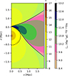Fig. 1. Distribution of the PDM density around a point mass in a homogeneous external gravitational field. The mass of the point source, located in the center of the coordinate system, is 1011 M⊙. The external field has the value of 0.02 a0 and points up. The left and right color scales indicate the positive and negative densities of PDM, respectively. The dotted half-circle marks the theoretical estimate of the radius ref below which the effects of the external field are negligible.

The region of the positive DM thus has asymptotically a bi-conical shape (see also Milgrom 1986). The direction of the external field is relatively easy to determine only for galaxies close to their massive neighbors or galaxy clusters (e.g., Haghi et al. 2016; Müller et al. 2019; Chae et al. 2020). Gravitational lensing in these situations are investigated in detail in Sect. 7. Some other properties of the distribution of the PDM for a point mass in a external field were described in Milgrom (2009), where their “surrogate phantom density” equals exactly to ρ_ph of QUMOND (Milgrom 2010).

6.3. Unknown direction of the external field

In this section, we aim to predict and explore the density profiles of PDM halos that would be inferred by a weak lensing analysis of stacked lenses, supposing that for each lens the external field has a random direction drawn from an isotropic distribution. As we explained in Sect. 3, the surface density we obtain in this way is the average surface density over all lenses. The average surface density ${\stackrel{\sim }{\mathrm{\Sigma }}}_{\mathrm{ph}}$ can be obtained by projecting the spherically averaged volume density as:

$$\begin{array}{c}\hfill {\stackrel{\sim }{\rho }}_{\mathrm{ph}}(r)=\frac{1}{4\pi r^2}{{\displaystyle \int }}_{\mathbb{S}(r)}{\rho }_{\mathrm{ph}}({\mathit{r}}^{\mathbf{\prime }})\mathrm{d}S.\end{array}$$(25)

We calculated the radial profiles of ${\stackrel{\sim }{\rho }}_{\mathrm{ph}}$ and ${\stackrel{\sim }{\mathrm{\Sigma }}}_{\mathrm{ph}}$ numerically for a point mass of the mass of 4 × 10¹⁰ M_⊙. We varied the magnitude of the external field between 0.005 − 0.07a₀. The results are plotted in the first two panels of Fig. 2. We also plotted the surface density of PDM in another scale in Fig. 3 to better illustrate the “ring of dark matter” phenomenon. The vertical dashed lines in these figures indicate the radius, r_M. The third panel of Fig. 2 shows the ratio of ${\stackrel{\sim }{\mathrm{\Sigma }}}_{\mathrm{ph}}$ to the surface density of an isothermal halo according to Eq. (22). The fourth panel shows the tangential shear. These results were calculated using Eq. (15), assuming the distances from Sect. 5. The radii r_ef are marked in Fig. 2 by the short horizontal bars on the corresponding curves. We can make note of several facts in these plots, as follows.

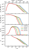Fig. 2. Stacked point masses in randomly oriented external fields. From top to bottom: Row 1: Density of PDM. Row 2: Surface densities obtained by the projection of the volume densities above. Row 3: Ratio of the surface density of the PDM halo and the surface density of the approximating isothermal sphere. Row 4: Tangential shear. The different lines correspond to the indicated various intensities of the external field. The small horizontal line on each curve marks the corresponding radius ref. For the given models, 1 kpc corresponds to 1.03″.

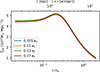Fig. 3. Detail of the central profile of the surface density of PDM.

1. The profile of the density or surface density of the PDM halo is strongly affected by the external field only in the regions that are further from the point mass than r_ef. We need to measure surface density with a precision better than about 10¹² M_⊙ Mpc⁻². The differences in the r_ef radii are in the order of hundreds of kpc for the range of external field magnitudes considered here.

2. Between r_M and r_ef, the external field reduces the surface density by about one to ten times compared to the isolated case described by Eq. (22).

3. Under the r_M radius, the external field does not affect the surface density substantially.

4. The spherically averaged density reaches a maximum at 0.26r_M, the surface density at 0.20r_M, with a change at third valid decimal place when the external field intensity ranges between (0.005–0.07)a₀. The position of the maximum can however be different for other interpolating functions, see Milgrom & Sanders (2008).

5. The ring of dark matter phenomenon occurs, for the assumed interpolation function, near the radius at which ϵ = 1, that is where strong lensing occurs and the weak lensing approximation is no longer precise.

6. The spherically averaged density of the PDM halo ${\stackrel{\sim }{\rho }}_{\mathrm{ph}}$ falls steeply beyond r_ef. This can already be recognized from Eq. (24) for the approximate asymptotic density of a PDM halo, since the integral of this expression over a sphere with a radius r is zero. We found numerically that

   $$\begin{array}{c}\hfill {\stackrel{\sim }{\rho }}_{\mathrm{ph}}\propto r^{-7},{\stackrel{\sim }{\mathrm{\Sigma }}}_{\mathrm{ph}}\propto r^{-6}\end{array}$$(26)

   for r ≫ r_ef. We can make a similar calculation to that in Appendix A to derive a general equation for the density of the PDM in the deep-MOND regime of any MOND theory which does not introduce any other new constant than a₀. The result is:

   $$\begin{array}{c}\hfill {\stackrel{\sim }{\rho }}_{\mathrm{ph}}(r)=\frac{1}{r^2}\sqrt{\frac{M{a}_0}{G}}f\left(\frac{g_{e}r}{\sqrt{GM{a}_0}}\right).\end{array}$$(27)

   For QUMOND, a comparison to Eq. (26) yields that f(x)∝x⁻⁵ for r ≫ r_ef, and, thus, we have:

   $$\begin{array}{c}\hfill {\stackrel{\sim }{\rho }}_{\mathrm{ph}}\propto \frac{1}{r^7}\frac{G^2{M}^3{a}_0^3}{g_e^5}\end{array}$$(28)

   in this region. We found (numerically) that the proportionality constant is close to (4π)⁻².

Equation (27) tells us how to rescale these results for points of different masses, as long as we are interested in the regions in the deep-MOND regime. For example, if we are interested in an object that is four times more massive than the fiducial one, we have to look for a curve for an external field that if two times stronger and than to multiply the values in the plot by two. Alternatively, we can have a look at a radius that is two times larger and divide the value which we read in the plot by four.

6.4. Comparison to an NFW halo

Between the radii r_M and r_ef, the density of PDM is roughly like of an isothermal sphere, given by Eq. (21). This is in contrast with the predictions of the ΛCDM cosmology, where DM halos are expected to have a density profile similar to the Navarro-Frenk-White (NFW) profile (Navarro et al. 1996). We thus could discriminate between the ΛCDM model and MOND if we could decide what profile of (phantom) dark halos galaxies have. We quantified the difference for one representative galaxy. We chose the baryonic mass of the galaxy as M = 4 × 10¹⁰ M_⊙, similar to the characteristic mass M_* of the galaxy mass function (Kawinwanichakij et al. 2020). Then we assigned a DM halo to the galaxy making use of the mean stellar-to-halo relation (Behroozi et al. 2013) and halo mass-concentration relation (Diemer & Kravtsov 2015) at zero redshift. This yielded the virial mass of the halo of 1.6 × 10¹² M_⊙ and a virial radius of 310 kpc. We studied the radial range only up to the virial radius (see, e.g., Diemer & Kravtsov 2015 for a more detailed behaviour of CDM halos at large radii).

We compared this NFW halo with the spherically averaged MOND PDM halos in Fig. 4 for several different magnitudes of the external field: the top panel shows the difference of the profiles of density, and the middle and bottom panel the same for surface density and tangential shear, respectively. For the calculation of the lensing effects, we used Eq. (15) and the distances from Sect. 5.

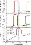Fig. 4. Comparison of a PDM halo to an NFW halo. The point mass has a baryonic mass of 4 × 1010 M⊙ and lies at the distance of 200 Mpc. Row 1: Difference of densities (the curves for ge = 0.005 a0 and 0.01 a0 nearly coincide). Row 2: Difference of surface densities. Row 3: Difference of tangential shears. The sources are assumed to be at infinity. The vertical dashed line indicates the MOND transitional radius rM.

The figure shows that for detecting the deviation of the PDM halo from the NFW halo need to detect a difference in surface densities on the order of 10¹³ M_⊙ Mpc⁻² or in tangential shears on the order of 10⁻³ in the radial range of tens of arcsec. We discuss whether such a measurement is feasible in Sect. 8. The deviation of the PDM halo from the NFW halo beyond about 100 kpc depends strongly on the magnitude of the external field.

7. Gravitational lensing by two point masses in MOND

Milgrom (1986) showed that there is a region of negative PDM between a pair of two masses near the point of zero acceleration. For the case of equal point masses, he derived, assuming the AQUAL version of MOND, an expression for the density of PDM in the plane going through the zero-acceleration point and is perpendicular to the line joining the point masses. He found that ρ_ph reaches an infinitely negative density near the symmetry axis since ρ_ph ∝ r^−1/2. The region of the negative PDM has a shape of the figure “8” rotating by its short axis around the line connecting the two point masses. In Sect. 7.1, we explore the distribution of PDM in more detail, assuming the QUMOND formulation of MOND. The weak lensing signature of QUMOND for this mass configuration is studied in Sect. 7.2.

7.1. Distribution of PDM around two point masses

In this section we investigate the distribution of PDM around a pair of point masses in a zero external field. Let us denote the masses of the two points by M₁ and M₂, such that M₁ ≥ M₂, and their distance by d. We work in the cylindrical coordinate system that has its axial coordinate, z coincident with the connecting line of the point masses. We denote the radial coordinate by r. Let the point mass M₁ be located at z = 0 and M₂ at z = −d. The density ρ_ph or projected surface density Σ_ph of the PDM at the position x can depend only on G, a₀, M₁, M₂, d and x. For dimensional reasons, ρ_ph and Σ_ph must be given by expressions of the forms:

$$\begin{array}{cc}\hfill {\rho }_{\mathrm{ph}}& =\frac{M_{\mathrm{tot}}}{d^3}f(\eta ,\theta ,\frac{\mathit{x}}{d})\mathrm{and}\hfill \\ \hfill {\mathrm{\Sigma }}_{\mathrm{ph}}& =\frac{a_0}{G}f(\eta ,\theta ,\frac{\mathit{x}}{d}),\hfill \end{array}$$(29)

where

$$\begin{array}{c}\hfill M_{\mathrm{tot}}=M_1+M_2,\eta =\frac{M_2}{M_1},\text{and}\theta =\frac{\sqrt{G{M}_{\mathrm{tot}}/a_0}}{d}.\end{array}$$(30)

The parameter θ quantifies how deep the system is in the MOND regime. In the following, we consider only situations where log₁₀θ > −3; this is because for lower values, a real system would probably be affected by the external field from the large-scale cosmic structures (Sect. 1). This is expected to happen approximately for θ < g_e/a₀, as we precise in Sect. 7.4. If we deal with regions of space where the gravitational acceleration is much less than a₀, then we can directly use Eqs. (3) and (4), with d signifying the distance between the point masses.

We derived the analytic expression for the density of PDM around two point masses without an external field, making use of Eq. 1. It is stated in Appendix D. Let us first explore the shape of the region of the negative PDM density. In Fig. 5 we plotted the PDM for two point masses that are in the distance of 200 kpc and various mass ratios η for M₁ = 10¹¹ M_⊙. The top row of the figure, showing the whole system, illustrates that with decreasing η the negative PDM region becomes smaller and gets closer to M₂. In the bottom row, the displayed region scales with the size of the region of the negative PDM. The images here show that the negative PDM region becomes bent towards the mass M₂ with decreasing η and the typical density of the region of negative PDM becomes more negative. Equation (29) allows for the maps of ρ_ph to be rescaled for different masses and separations of the point masses.

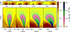Fig. 5. Distribution of the PDM around two point masses (zero external field assumed) with various mass ratios indicated above each column. The mass of M1 is 1011 M⊙ and the two point masses are 200 kpc apart. The mass ratio is the same for each column. The top row shows the whole system, in the bottom row we can see magnified the region of the negative PDM. Note that the vertical ranges of the plots in the bottom row are different for each plot. In each plot, the r and z axes have the same scale.

The characteristic signature of MOND is the region of the negative PDM. For its detection by weak lensing it is useful to know its size. We now prove a noteworthy fact that as long as the interpolation function ν is monotonically decreasing, the shape of the region of negative PDM in QUMOND is given by a fully Newtonian expression, that is that the expression does not contain the MOND constant a₀ or the interpolation function. This actually holds true for any configuration of matter, as long as we are concerned with the regions where the density of the real matter is zero. Indeed, using Einstein’s notation, Eq. (1) gives outside the distribution of the real matter that:

$$\begin{array}{c}\hfill -4\pi G{\rho }_{\mathrm{ph}}={\partial }_i\left[\nu g_N^i\right]={\partial }_i(\nu )g_N^i+\nu {\partial }_i{g}_N^i=\frac{{\nu }^{\prime }}{a_0}{\partial }_i{(g_N^j{g}_{N,j})}^{1/2}{g}_N^i.\end{array}$$(31)

In the last expression, the first factor can only be negative, and therefore the surface where ρ_ph = 0 is given by the other two Newtonian factors.

We characterize the shape of the negative PDM region by its maximum radial extent r_max and its minimum and maximum z coordinate with respect to the position of the mass M₂ (i.e., z_min = 0 indicates that the minimum z coordinate is reached at z = −d). It follows from the previous paragraph that any linear dimension of this region, x, depends only on G, M₁, M₂, and d. A dimensional analysis then indicates that x/d = f(η). We derived the function numerically for r_max, z_min and z_max and is shown in Fig. 6. The value of z_min becomes negative for η < 3.91 × 10⁻³.

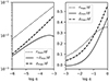Fig. 6. Dimensions of the region of negative PDM.

Next, let us focus on the mass and characteristic surface density of the region of negative PDM. A dimensional analysis gives that the mass of the region, M_neg, satisfies M_neg/M_tot = f(η, θ). We calculated the function numerically in the top panel of Fig. 7. It is interesting that the mass of the negative region can be comparable, or even higher than the total baryonic mass of the system. This happens preferably for systems consisting of two similar masses in deep-MOND regime. For example, for two galaxy clusters with a mass of 10¹³ M_⊙ located 15 Mpc apart, the θ parameter is about 10⁻² and therefore the region of negative PDM would have a mass of a galaxy cluster.

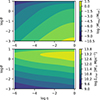Fig. 7. Mass and characteristic surface density of the region of the negative density of PDM. Top: Mass of the region of the negative density of PDM in the units of the total baryonic mass of the system Mtot = M1 + M2 as a function of the parameters η = M1/M2 and $\theta =\sqrt{G{a}_0{M}_{\mathrm{tot}}}/d$. Bottom: Characteristic projected surface density of the region of the negative PDM.

The surface density depends on the particular configuration of the problem and orientation with respect to the line of sight. We explore some particular situations in detail in Sect. 7.2. Here we study only the characteristic surface density of the region of the negative PDM to get an order-of-magnitude estimate and investigate how it scales with η and θ. In particular, we defined Σ_char = M_neg/[2r_max(z_max−z_min)]. It is plotted in the bottom panel of Fig. 7 as a function of η and θ. The figure indicates that the characteristic surface density depends primarily on θ and that it reaches a maximum at η = 1 and θ ≈ 2.5, i.e. for equal-mass systems near the border of the Newtonian and deep-MOND regime. This is similar to the case of the surface density of the PDM around a point mass, which reaches the maximum near the border of the Newtonian and deep-MOND regions. For example, for two equal galaxies with a mass of 10¹¹ M_⊙ (comparable to the Andromeda galaxy), θ = 2.5 corresponds to a distance of 6 kpc. Such galaxies would be interacting. Figure 6 shows that the radius of such a region would be about 3 kpc.

Next, we explored the limit behavior of ρ_ph close to the zero-acceleration point located at (r, z) = (0, z₀) where $z_0=-d/(1+\sqrt{\eta })$. After calculating the second-order Taylor expansion of the expression for the Newtonian gravitational potential around the zero-acceleration point, and making use of the fact that ν(x)∼x^−1/2 for small arguments, from Eq. (1), we get:

$$\begin{array}{cc}\hfill {\rho }_{\mathrm{ph}}& \sim \frac{{(\sqrt{M_1}+\sqrt{M_2})}^2}{8\pi d^{3/2}{(M_1{M}_2)}^{1/4}}\sqrt{\frac{a_0}{G}}\frac{8{(z-z_0)}^2-r^2}{{[4{(z-z_0)}^2+r^2]}^{5/4}}\hfill \\ \hfill & \text{for}(r,z)\to (0,z_0).\hfill \end{array}$$(32)

Thus, if we approach the zero-acceleration point perpendicularly to the z axis, ρ_ph reaches a negative infinity like r^−1/2. The same was shown for the AQUAL formulation of MOND by Milgrom (1986). On the other hand, when we approach the zero-acceleration point along the line r = 0, ρ_ph reaches the positive infinity like (z − z₀)^−1/2. Interestingly, this holds true even if the point masses are close to each other, such that the system is in the Newtonian regime.

While the volume density of PDM is diverging around the zero acceleration point, in Appendix B, we prove that the projected surface density near this point is finite. So far, it has only been proven that there is an upper limit on the surface density of PDM halos of nearly spherical objects (Milgrom 2014a).

7.2. Pair of point masses observed perpendicularly

Lensing analyses are based on observations ellipticity, position angles and magnifications of the lensed sources. A map of these quantities can be converted to the map of surface density (e.g., Kaiser & Squires 1993). In this section we provide these maps for a pair of point masses predicted by MOND. In this first investigation of the topic, we consider just two orientations of the point masses with respect to the observer: the perpendicular view and the axial view. Furthermore, we consider lensing by what we call the superposition density. This is the density which is obtained by assigning the point masses the spherically averaged PDM densities ${\stackrel{\sim }{\rho }}_{\mathrm{ph}}$ derived in Sect. 6, that are expected by for single point masses in the respective external field, and summing them. The difference of PDM density and the superposition density quantifies a key property of MOND, namely its non-linearity, by which it differs from the Newtonian gravity. In addition, we propose to test MOND by subtracting the weak lensing signal observed around solitary point masses from the lensing signal observed around pairs of point masses and to compare the result to the MOND predictions predictions. A similar approach is used for example for detecting the lensing signal of the cosmic filaments connecting galaxy groups (Epps & Hudson 2017; Yang et al. 2020). In such a test, it would be necessary to ensure that the solitary point masses and pairs of point masses reside in equally strong external fields. In Sect. 8, we discuss the prospects of detecting the specific signatures of QUMOND observationally.

7.2.1. Computational methods

Let us start with the case that the point masses are observed perpendicularly to their connecting line. We calculated the surface density map simply by integrating numerically the expression for the PDM of a pair of point masses in Appendix D:

$$\begin{array}{c}\hfill {\mathrm{\Sigma }}_{\mathrm{ph}}={\displaystyle {\int }_{-Y}^Y}{\rho }_{\mathrm{ph}}(x,y,z)\mathrm{d}y.\end{array}$$(33)

We note that the expression for ρ_ph does not involve the external field. In the following, we took into account the value of the external field g_e approximatively through the limit of the integral, Y. In particular, we integrated between the outermost points where the Newtonian acceleration generated by the point masses was equal to the Newtonian external field, g_e, N, a number obtained by solving Eq. (19) for g = g_e. In other words, we took into account only the PDM located in the region where the total gravitational field is dominated by the contribution of the point-mass pair. Consequently, Σ_ph was considered non-zero only in a limited region of space. This approximation is justified in Sect. 7.4. It is related to the finding from Sect. 6 that the density of PDM drops quickly outside the region dominated by the internal field. We refrained in this first investigation of the topic the averaging of ρ_ph over all possible directions of the external field, like in the case of a solitary point mass in Sect. 6, because of high computing demands.

In order to calculate lensing maps, we had to solve the 2D Poisson equation, Eq. (5), for the lensing potential. This was done by numerically by convolution of Σ_ph with the lensing potential of a point mass given by Eq. (8) and adding the contributions of the real matter. To make the computation feasible, we progressed in a zoom-out fashion. First, the potential was calculated on a fine grid in the region depicted in the maps. Then it was necessary to add also the contributions to the lensing potential coming from the outside of this region. In the second step, we thus defined a grid that was twice as large as the previous one, had the same number of grid nodes, and had the same center. The nodes that were covered already by the previous grid were assigned a zero surface density and the others the correct density Σ_ph. The lensing potential at this grid was again calculated by convolution. We repeated this procedure until we covered the region of non-zero Σ_ph completely. We added also to the surface density the contributions of the point masses themselves once they got covered by the expanding grid. In this way, the contributions to the lensing potential from various spatial scales were contained in several layers. At the end, the lensing potential in each layers was interpolated for the grid points of the densest grid and the resulting lensing potential was obtained by summing up the contributions from all layers. The correct functioning of the code was verified by comparison with analytic solutions for the lensing potential for various combinations of point masses and isothermal spheres. Numerical derivatives were used to obtain the Jacobian matrix from the lensing potential according to Eq. (9).

For the axial configuration, i.e. when the two point masses lie along the same line of sight, we obtained the surface density of the PDM in a similar fashion:

$$\begin{array}{c}\hfill {\mathrm{\Sigma }}_{\mathrm{ph}}={\displaystyle {\int }_{Z_1}^{Z_2}}{\rho }_{\mathrm{ph}}(x,y,z)\mathrm{d}z.\end{array}$$(34)

The limits of the integral were again chosen as the minimum and maximum z-coordinate at which, for a given x and y, the Newtonian acceleration generated by the two point masses was equal to g_e, N. Given that this density distribution is axially symmetric, we could use the simple Eq. (15) to obtain the tangential shear. Some aspects of gravitational lensing for this configuration of matter have already been investigated by Milgrom & Sanders (2008). Unlike we do here, they used an approximate formula for the density of PDM and focused on the influence of the choice of the MOND interpolation function.

7.2.2. Explored sample of models

The models that we explored were variations of a fiducial model. It is fully characterized by the dimensionless parameters θ = 0.1, η = 0.4 and g_ext = 0.03a₀ and the mass of the more massive point of M₁ = 10¹¹ M_⊙. This implies the mass of the lighter point M₂ = 4 × 10¹⁰ M_⊙ and the distance between the points of d = 127.4 kpc. We assume the distances of the lenses and sources as described in Sect. 5. This results in the angular separation of the two point masses of 2.18′.

The other explored models were obtained by varying of one of the parameters η, θ or g_ext of the fiducial model while keeping the other parameters intact. In particular, the explored values were η = [0.1, 0.16, 0.4, 1], θ = [0.06, 0.1, 0.3, 1], g_ext/a₀ = [0.005, 0.01, 0.03, 0.07]. The separation of the points of varied as [212.4, 127.4, 42.5, 12.7] kpc when varying θ and as [113.0, 116.0, 127.4, 152.3] kpc when varying η. At the assumed lens distance, one kpc is almost exactly one arcsecond and the critical density comes out log₁₀Σ_cr/(M_⊙ Mpc⁻²) = 15.92, which can be used for converting the surface density into the lensing magnification with the aid of Eq. (17). We can rescale the results to other configurations of the problem using the relations Eq. (3) and Eq. (4) and the results of Sect. 4.

7.2.3. Results

The figures discussed in this section are available at Zenodo¹ and at Astro-ph².

Figures Sigmachange-wide.pdf and Sigmachange-zoom.pdf show the surface densities of PDM around the considered models from the perpendicular view. The former figure shows for all models the whole halos, while the latter shows the vicinity of the point masses. The plots showing the fiducial model are marked by the red frames. The sizes of the displayed regions in the zoomed-in plots are proportional to the distances between the point masses by a constant factor. The size of the PDM halo in the fiducial model, beyond which the halo is expected to be truncated, is around 500 kpc. This size only mildly depends on the choice of η or θ, but decreases strongly with increasing g_ext. The outline remains in all cases nearly circular, except in the model with the strongest g_ext, when the halo becomes elongated along the line connecting the point masses. All parameters influence noticeably the inner morphology of the halo, as evident from Fig. Sigmachange-zoom.pdf.

The region of the negative PDM density has its counterpart in as a dip in the surface density. Nevertheless, the surface density is not necessarily negative – the contribution of negative density near the zero acceleration point is balanced by the contribution of the positive density from the regions which are further away from the symmetry axis. The surface density can be negative if the system is exposed to a strong-enough external field. This is because the external field reduces the contribution of the positive PDM do the surface density that otherwise occupies the external regions of the system. The surface density becomes negative also for very low acceleration systems (i.e., the θ parameter is low). In this case, the positive contribution of the outer part of the PDM halo, whose mass is given by the masses M₁ and M₂ and the value of the external field, is overweighted by the large amounts of negative PDM near the zero acceleration point. Indeed, if the distance between the two point masses is large, then θ is small and Fig. 7 indicates that the mass of the region of the negative PDM is large.

The magnitude of the dip is generally a factor of a few. For the fiducial model, the dip occurs at the surface density level of about 10¹³ M_⊙ Mpc⁻². This surface density grows the strongest with the θ parameter. This is because the density of PDM is the highest near the MOND transitional radius³ (Sect. 6) and the points become closer to each other with decreasing θ. We note that even if the PDM density diverges near the zero acceleration point (Eq. (32)), the surface density does not, as proved analytically in Appendix B.

Another characteristic feature which we see in Fig. Sigmachange-zoom.pdf is the offset outer halo of the less massive point. This is best visible in the top-left panel, showing a pair of a high mass ratio. One might look for such an affect for galaxies close to galaxy clusters.

Surface density difference. Figures SigmaDiffchange-wide.pdf and SigmaDiffchange-zoom.pdf show the difference between the PDM surface density and the superposition surface density, in order to explore the effect of the non-linearity of MOND. The first figure is again the complete view of the whole PDM halo, while the second shows only the central region around the point masses. The difference is negative near the center of the halo, meaning that the superposition surface density is higher than the true PDM surface density. This is because the amount of PDM around one of the point masses, compared to the case that the point mass were isolated, is reduced by the EFE imposed the other point mass. We note that the reduction of the surface density between the two point masses is the opposite of what we expect if the galaxies were connected by a cosmic filament (Yang et al. 2020).

On the other hand, the superposition surface density is less than the true PDM surface density in the outer parts of the halo. This is caused by the external field in which the point masses are embedded both: the combined PDM halo of the pair of point masses is truncated by the EFE at a larger radius, than the PDM halos of the single point masses that form the superposition halo. We note that in the external parts of the halo, the difference is relatively constant, having the value of around 10¹² M_⊙Mpc⁻².

In theories based on the assumption of particle DM and Newtonian gravity, the real density and superposition density will differ too, but probably in a different way. During the first approach of the two halos toward each other, the tidal force will bulge the halos along their connection line, producing a surplus of DM in between of the galaxies. Later, once the halos experience tidal stripping and compactification, the result is more difficult to predict. Nevertheless, Pawlowski et al. (2017) inspected the distribution of satellites around isolated pairs of galaxies in a ΛCDM simulation and found that they tend to be lopsided toward each other. In contrast, Fig. SigmaDiffchange-zoom.pdf shows that the PDM halos in QUMOND appear “squashed” in the region between the point masses. Here, the density of PDM is reduced compared to the superposition density, see Fig. SigmaDiffchange-zoom.pdf. At least this is true for the surface densities. Figure 5 shows that the volume density contours of PDM halos have more intricate shapes.

Lensing shear. Figures gamma1change.png and gamma2change.png show the maps of the real and imaginary part of the shear, respectively. The influence of the changes of the different parameters of the models is theoretically understood easier in the terms of the ellipticity magnitude and position angle, which demonstrate below. However, the shear components have the advantage over the ellipticity magnitude and position angle that they average when stacking different lenses.

Lensing ellipticity. Figure LensEllipchange.png presents the maps of lensing ellipticity for our models. For each model, there are three maxima of ellipticity: two near each of the point masses, and one near the zero-acceleration point. The detection of this last peak would be clear evidence of modified gravity. This peak is absent in Newtonian gravity for spherical DM halos, as we detail below. The first column of the figure demonstrates that the position the zero-acceleration peak depends on the mass ratio of the two point masses. The magnitude of the peak does not seem to significantly depend on the mass ratio of the point masses for the range of models considered here. Figure 8 depicts for the fiducial model the profile of the real component of the shear along the line connecting the two point masses. Because the imaginary part is much smaller than the real part, the plotted quantity, in absolute value, corresponds to the lensing ellipticity. It shows that for detecting the feature, the measurement of ellipticity has to reach the precision of 10⁻³ on the angular scale of 0.1′.

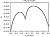Fig. 8. Profile of the real part of the shear along the line connecting two point masses in the fiducial model. The imaginary part is negligible over the plotted range.

The second column of Fig. LensEllipchange.png shows that the lensing ellipticity increases as the two point masses are becoming closer to each other. This can be understood in the following way. Equation (4) tells us that surface density of the PDM is proportional to d⁻¹ as long as we deal with a system in a deep-MOND regime, which means, in the present situation, as long as the separation between the point masses is much greater than the sum of their MOND transitional radii. Then, the linearity of Eqs. (5) and (12) implies that lensing ellipticity is proportional to d⁻¹ too. The last column of Fig. LensEllipchange.png indicates that the lensing ellipticity in the vicinity of the point masses varies only very little for the range of the strengths of the external field considered in this study. This is because the surface density of PDM plus baryonic matter, which is determines the lensing effects (Eq. (5)), depends most on the inner, that is the densest part of the PDM halo. The external field removes only the outer, little dense part of the PDM halo.

Lensing position angle. Let us turn to Fig. LensPAchange.png which shows the maps of the position angle of the lensing shear ellipses for our models. The position angle of 0 or 180°correspond to the orientation along the horizontal direction. The figure shows that the shear ellipses near the zero acceleration point are always elongated perpendicularly to the line connecting the point masses. In spite of the divergent and discontinuous nature of the PDM density near the zero acceleration point (Eq. (32)), the lensing effects are finite and continuous. It is striking that the maps of positional angle are virtually identical for all models in the second and third column. In the second column the distance between the point masses in kpc or arcmin varies, but displayed portion of the sky is proportional to the distance of the point masses. As before, we can use Eqs. (4), (5), and (12) to explain why the maps of shear positional angle do not depend on the separation of the point masses. The separation affects the lensing potential only as a multiplicative factor and thus only the magnitude of the complex shear is affected (i.e. the ellipticity), but not its phase (i.e. the positional angle). As before, the external field effect only affects the low-density regions of the PDM distributions, that are contribute only little to the surface density of the PDM, and therefore the maps of positional angle do not vary noticeably in our models when varying the intensity of the external field in the third column of Fig. LensPAchange.png.

Lensing shear difference. A key property of MOND is that the gravitational fields of two objects do not add up. In Figs. gamma1Diffchange.png and gamma2Diffchange.png we show the difference between actual shear expected by QUMOND and that stemming from the superposition density. The difference is on the order between about 10⁻⁴ and 10⁻², both for the real and imaginary components. Again, we aim to understand the behavior of with variations of the different parameters theoretically in the following paragraphs in the terms of lensing ellipticities and position angles.

Lensing ellipticity difference. Figure LensEllipDiffchange.png shows the differences in ellipticity caused by the PDM density and ellipticity caused by the superposition density. The difference is the highest when the point masses are the closest to each other. These maps emphasize the peak of ellipticity near the zero acceleration point, since this peak is absent in the superposition model. The peak in these ellipticity difference maps is on the order of 10⁻². The spatial size of the peak is roughly proportional to the distance between the point masses. The external field effect, at least within the range considered in this work, has again no appreciable impact on the result.

Lensing position angle difference. The differences between the shear positional angle caused by the PDM density and the superposition density are displayed in Fig. LensPADiffchange.png. In most regions, the difference of the position angles is a few degrees. Near the zero acceleration point, the positional angle difference is close to zero. The misalignment that is the easiest to detect observationally is around ninety degrees. There are indeed such regions; however, a comparison of Figs. LensEllipchange.png and LensEllipDiffchange.png reveals that this happens only where both that the actual and superposition ellipticities are close to zero, which is unfortunately where it is the most difficult to measure the positional angle. In order to simplify the comparison with Fig. LensEllipchange.png we drew in the upper halves of Fig. LensPADiffchange.png the contours of constant lensing ellipticity from Fig. LensEllipchange.png as the dotted lines. The contours in are at the ellipticity levels of 10⁻², 10^−2.5 and 10⁻³. The deviation of a few tens of degrees is encountered at the ellipticities of a bit above 10⁻³. For close pairs (high θ), the situation is more positive, because the ellipticites can be around 10⁻², but only at in a very small region of space.

Unlike for the positional angle, the difference of the positional angles of the true and superposition PDM shows a dependence on the distance between the point masses. This is because the superposition PDM is a construct that is inconsistent with MOND, such that Eq. (4) does not hold true for it because the superposition density does not obey the space-time scaling symmetry.

7.3. Pair of point masses observed aligned

We now turn to the case of two point masses observed along their connecting line, elaborating the results of Milgrom & Sanders (2008). The projected surface density for this orientation is axially symmetric, therefore, we focus only the radial profiles of surface density and tangential shear. We explored the same set of models as for the perpendicular view, as described in Sect. 7.2.2.

Surface density. The results for surface density are presented in Figs. TPM-LOS-Sigma_all-nogrid.pdf and TPM-LOS-Ellip_all-nogrid.pdf. The profile shows, similarly to the case of a single point mass, a peak near the MOND transitional radius, forming a ring when observed on the sky (Milgrom & Sanders 2008). The surface density of the PDM near the ring is about 10¹⁵ M_⊙ Mpc⁻². The height of the peak grows with the η parameter, since the total mass of the system increases. Increasing the θ parameter (i.e. decreasing the separation between the point masses while keeping their masses fixed), leads to a decrease of the surface density at a given distance from the origin⁴. This is because the gravitational field of one point mass is progressively more reduced by the external field effect coming from the other point mass, as θ increases, such that the density of the PDM decreases. If the point masses are far from each other, such that they reduce the gravity of each other the least, then Eq. (22) tells us that the surface density is proportional to $\sqrt{M_1}+\sqrt{M_2}$. In the opposite limit, when the two point masses coincide, the same equation indicates that the surface density is proportional to $\sqrt{M_1+M_2}$, that is lower. The strength of the external field again only has a negligible impact on the appearance of the inner profile of the PDM halo.

Surface density difference. The difference of the surface densities of PDM and the superposition density, shown in the bottom row of Fig. TPM-LOS-Sigma_all-nogrid.pdf, is generally on the order 10⁻¹³ M_⊙ Mpc⁻². Surprisingly, this is rather universal value valid for all radial distances from the symmetry center and for most of the explored models. The shapes of the profiles beyond about 10⁰ − 10¹ kpc are caused by the same effects as discussed for the perpendicular configuration. Near the center of symmetry, the superposition surface density can be both higher or lower than the superposition surface density. To see why, we note in Fig. 2 for a single point mass, that the density of the PDM around the point mass is falls steeply toward zero. The surface density near the point mass is therefore determined by the density further away from the point mass. If two point masses seen along the line-of-sight are close to each other (i.e., low θ), the external field of one of them reduces the volume density of the PDM of the other point mass. This phenomenon is absent for the PDM density and therefore its surface density can be higher than that of the actual PDM if the point masses are close to each other. On the other hand, if the point masses are far apart, the regions close to each of the point masses are almost equal to the superposition densities. Nevertheless, the combined gravitational fields of the two point masses resist easier to the global external field than if the point masses were isolated. Thus, in this case, the superposition PDM surface density is lower than the actual PDM surface density. The enhanced resistance of the actual PDM density to the global external field, when compared to the superposition PDM density, explains the behavior for the varying intensity of the global external field.

Tangential shear. In Fig. TPM-LOS-Ellip_all-nogrid.pdf, we can see that the radial profiles of tangential shear are rather featureless. They are approximated well by a power law with a slope close to 1.5, a value in between of what we expect for a point mass and an isothermal PDM halo, see Eqs. (15) and (22). The tangential shear increases at a fixed radius with increasing η, because the total baryonic mass of the system increases. With increasing θ, the tangential shear decreases as the PDM density of one point mass is becomes diminished by the EFE coming from the other point, which is located closer. The global external field manifests itself virtually only as a truncation of the PDM halo at larger projected galactocentric radii.

Tangential shear difference. The differences in the true tangential shear from the tangential shear expected from the superposition density is on the order of 10⁻⁴, as we can see in the bottom row of Fig. TPM-LOS-Ellip_all-nogrid.pdf. The explanation of the behavior of the curves when θ and the global external fields are varied is the same as for the case of the surface density.

7.4. Influence of external field

In this section, we briefly explore the influence of an external field on the distribution of PDM around a pair of point masses. We also discuss the correctness of the simplified treatment of the external field in Sect. 7.2 on the prediction of gravitational lensing. We work in a Cartesian coordinate system whose z axis is defined as before (Sect. 7.1) and the x and y axes are chosen such that the coordinate system is right-handed. We derived an analytic expression for the density of PDM. It is stated in Appendix E. It allows for an arbitrary orientation of the external field.

For the purpose of the discussion of the accuracy of the details in Sect. 7.2, here we introduce a parameter that characterizes how important the external field is for the density of the PDM between the two point masses. We expect that the distribution of the PDM will be relatively unaffected in the region where the intensity of the internal field of the system will be weaker than the intensity of the external flied, g_e. The size of this region, r, thus approximately satisfies $\sqrt{G{M}_{\mathrm{tot}}{a}_0}/r\approx g_e$. We expect that the region between the point masses starts being affected by the external field once r becomes smaller than d, which is equivalent to θ < g_e/a₀. This leads us to the introduction of the τ parameter,

$$\begin{array}{c}\hfill g_e/a_0=\tau \theta ,\end{array}$$(35)

which is expected to be much less than one if the impact of the external field on the distribution of PDM between the two point masses is negligible, and much greater than one when the impact of the external field is substantial. We verify this below.

In Fig. 9, we show the variations of the density of PDM in our fiducial model (Sect. 7.2.2) when the system is embedded in a homogeneous external field of different directions and intensities. The intensities are quantified through the parameter τ. In the depicted models, τ = 1 corresponds to the external field of g_e = 0.1a₀. Figure 10 shows the same but the displayed region is zoomed in to the vicinity of the two point masses. In this figure, in addition there is a white circle of the radius of 5 kpc that is centered on the zero-acceleration point of the fiducial model without the external field. The dotted lines indicate the borders of the region of isolation defined as in Sect. 7.2.1, where we used it to determine the limits of the integral for calculation of the surface density of the PDM. Figure 11 shows the ratio of the models with external field to the model without the external field from Sect. 7.2.3. We can make several observations in these figures.

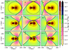Fig. 9. Pair of point masses in an external field. The image shows the density of the PDM in a plane going through the point masses. Different columns correspond to different directions of the external field. The direction is indicated by the arrows. In each column, the magnitude of the external field is stronger with each tile downwards. The magnitude is specified through the τ parameter defined by Eq. (35). The dashed curves indicate the surfaces within which we neglected the EFE in Sect. 7.2. The full black lines indicate the boundaries between the regions of positive and negative density of the PDM.

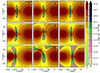Fig. 10. Same as Fig. 9, but only the near vicinity of the point masses is shown. The white circle indicates the position of the zero-acceleration point in the situation without an external field. The radius of the circle is 5 kpc.

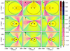Fig. 11. Ratio of the densities of PDM around two point masses without and with the external field. The meaning of the different tiles is the same as in Fig. 9.

Figures 9 and 10 show that the density of PDM is only little affected by the direction of the external field in the region of isolation. Figure 10 shows that this density in this region is almost the same as if the external field was neglected. This justifies the integrand of Eq. (33). The limits of the integral in Eq. (33) are justified by our results from Sect. 6 that after averaging the PDM densities over all possible directions of the external field, the density steeply decreases beyond the outer border of the region of isolation.

In contrast, just beyond the region of isolation the density of PDM depends strongly on the intensity and direction of the external field. It is noteworthy that the external region of negative PDM density always nearly touches the region of isolation. Far from the point masses, the distribution of PDM approaches that of a single point mass in an external field (Eq. (24)).

It is interesting to note that the external field does not much modify the absolute value of the density of the PDM outside of the region of isolation; rather only its sign. The external field effect thus seems to arise from a large part because of the influence of the regions of the negative PDM density, that mitigate the influence of the regions of the positive PDM density. This is a hypothesis that needs a more careful analysis in future works. When averaging over various directions of the external field, the contributions of the positive and negative densities of PDM almost cancel each other, which explains the steep decline of the curves in Fig. 2 beyond the r_ef radius. This is hinted also by Eq. (24), whose spherical average is zero at any radius.

The figures reveal that the parameter τ indeed characterizes the importance of the external field on the distribution of the PDM between the pair of point masses, in agreement with the above order-of-magnitude estimates. We verified that this is the case also for models with different values of θ and η. At τ = 1.5, the density of PDM between the two point masses is strongly affected by the external field. It is difficult to predict what would be the average PDM density in this region when averaging over all possible directions of the external field. This is the reason why we avoided strong external fields in Sect. 7.2 or very separated point masses in the predictions for gravitational lensing, given that we used an approximate method. The greatest value of τ used in our lensing models (Sect. 7.2.3 and Sect. 7.3) is 0.7.

The external gravitational field should be dominant also around the point of zero internal acceleration. From this perspective, it is interesting that the “8” shaped region of negative PDM near the zero acceleration point is not much influenced by the external field as long as τ ≲ 1. The position and size of the region vary just by several percent. In weak lensing counterpart of this region will then be just mildly blurred by the varying direction of the external field, as long as the τ < 1.

8. Observational aspects

Here we comment on the observational aspects of the detection of the signatures of QUMOND gravity in weak lensing analysis. First, in MOND, for certain interpolation functions, PDM halos can have central cavities (Sect. 6). This might have already been observed for one galaxy cluster (Jee et al. 2007; Milgrom & Sanders 2008). It would be desirable to look for similar rings of DM also in other objects. Let us turn to galaxies as the lenses. If the effects of the central cavity of the PDM halo are visible only close to the centers of the galaxies, the body of the galaxy might make the determination of the shapes of the background galaxies difficult and therefore practically disable the test. Here we focus on early-type galaxies, because the situation might be much more difficult for the spirals, which contain a lot of substructure. In Fig. 12 we compared the effective radii of early-type galaxies from the ATLAS^3D sample (Cappellari et al. 2011) to their MOND transitional radii r_M. We estimated the baryonic masses of the galaxies as the dynamical masses within 1r_e published in Cappellari et al. (2013) multiplied by 0.87, to account for the small contribution of DM to the dynamical mass (Cappellari et al. 2013). Figure 12 shows that the MOND transitional radius is typically three times larger than effective radius. Let us assume, as a rough estimate, that we can detect background sources which are projected further away from the galaxy center than the effective radius (after subtracting its model, probably). Figure 3 indicates that we would not be able to detect the ring of dark matter effect. In this regard, quiescent galaxies at high redshifts are more promising, because at a fixed stellar mass, they are a few times smaller than their local counterparts (e.g., Trujillo et al. 2006, 2011; Damjanov et al. 2011). Nevertheless, one might also inspect the deviation of the observed density profile from the isothermal sphere. The third and fourth panel of Fig. 2 indicate that the central deviation might be observable even for galaxies meeting the local mass-size relation.

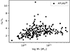Fig. 12. Comparison of the MOND transitional radii rM to the effective radii re of the early-type galaxies from the ATLAS3D survey.

In Fig. 4, we inspected the deviation of the QUMOND-predicted profile of the PDM from the profile expected in the ΛCDM cosmology for NFW halos. Actually, it has already been shown recently that the halos of isolated galaxies prefer MOND over NFW halos (Mistele et al. 2024a). It would be interesting to inspect whether the ratio of the observed surface density to the surface density of the MOND isothermal PDM halo (Eq. (22)) shows the curvature because of the EFE, as seen in the fourth panel of Fig. 2.

Next, let us consider the number of lenses that we need in order to detect the specific signatures of QUMOND. Bartelmann & Maturi (2017) give several useful numbers and formulas. If we have a spatial bin containing N_b background galaxies, the uncertainty of the measurement of complex ellipticity projected to some coordinate axis, δϵ, can be estimated as $\delta ϵ={\sigma }_{ϵ}/\sqrt{N_{\mathrm{b}}}$ where σ_ϵ = 0.2. The number of the background sources can be expressed as N_b = n S​N_L if n denotes the number of the background sources per square arcminute, S the angular area of the bin and N_L the number of the stacked lenses. Combining these two equations, we get

$$\begin{array}{c}\hfill N_{\mathrm{L}}=\frac{{\sigma }_{ϵ}^2}{nS\delta {ϵ}^2}.\end{array}$$(36)

Bartelmann & Maturi (2017) state that n = 30 − 50 galaxies per square arcminute for images by space-based telescopes. In the examples below, we assume the optimist value n = 50 arcmin⁻². The recently launched Euclid satellite is expected to have similar capacities and will cover one third of the extragalactic sky.

In Fig. 4, we see that the QUMOND tangential shear for the considered model differs from the tangential shear in ΛCDM in the radial range of ca. 4–20″. The difference is 10⁻³. If we use all background galaxies in such an annular aperture, we need to stack 2400 lenses for a one sigma detection of this feature, or nine times as much for a three sigma detection.

For the fiducial model of the pair of point masses in the perpendicular view, the γ₁ dip at the zero-acceleration point has the size of about 0.1 × 0.1′ and is depressed by about 10⁻³ below its neighborhood (Figs. 8 and LensEllipchange.png). Its one sigma detection thus requires 40 000 lensing pairs. For comparison, the catalog of isolated galaxy pairs of Nottale & Chamaraux (2018) contains just 13 000 items. In order to detect this feature, a larger catalog of lenses would have to be constructed. Galaxy cluster pairs might be more suitable.

It would be easier to look for the deviation of the actual shear from the shear resulting from the superposition density. The latter can be constructed empirically, by investigating the lensing around isolated galaxies, similarly to Brouwer et al. (2021) or Mistele et al. (2024a). Figures gamma1Diffchange.png and gamma2Diffchange.png show that the difference is on the order of 10⁻³ over the area of about eight square arcminutes for our fiducial model. Only 100 lenses are needed for a one sigma detection. As explained in Sect. 7.2.3, in Newtonian gravity with particle DM, the action of close-by DM halos on each other is probably qualitatively different from the PDM halos in QUMOND.

Finally, let us mention some general potential caveats of similar studies. When determining the baryonic masses of the lens galaxies, one should take into account also the masses of the circumgalactic media (see, e.g., Mistele et al. 2024a). It can be substantial even for the Milky-Way type galaxies (Gupta et al. 2012). The catalogs like that of Nottale & Chamaraux (2018) define the isolation in another way than considered here. Namely, they demand the third nearest galaxy to be some multiple of the projected separation of the pair in question. In the present paper, we instead required a homogeneous and rather weak external field. In the catalog of Nottale & Chamaraux (2018) there are some obvious members of galaxy clusters. The two galaxies in the pair just have similar velocities, that are much different from the velocities of the other nearby cluster members. Pairs of nearby galaxies or galaxy clusters can be connected by a cosmic filament (Epps & Hudson 2017; Yang et al. 2020), which could interfere with the sought effects. Also, it should should be stressed that the numbers of necessary lenses given above reflect only the statistical error stemming from the random orientation of the background galaxies. Actually, more lenses might be needed because of other uncertainty sources, such as determining the masses of the galaxies, their distance from the observer, or in the case of object pairs, the distances with respect to each other that are subject to the projection effect.

9. Conclusions

We expect different gravitational lensing around galaxies (or their clusters) for different solutions to the missing mass problem. Here we investigated in detail the distribution of the PDM around point masses and their pairs in the QUMOND version of MOND, while retaining the possibility to test the theory via weak lensing. All resulting maps are available at Zenodo⁵ and at Astro-ph⁶. The results are as follows.

9.1. Results for a point mass

• The external parts of a PDM halo of a point mass in an external field are offset with respect to the point mass away from the direction of the external field. This is visible in Fig. Sigmachange-zoom.pdf.

• We derived an analytic expression for the PDM density for this problem (Appendix C).

We considered the radial profile of a PDM halo of a point mass in an external field averaged over all lines of sight. This is the profile that is obtained by stacking of many objects embedded in external gravitational fields of random directions.

• As detailed by (Milgrom 2013), between the radii of around r_M (Eq. (20)) and r_ef (Eq. (23)), in the absence of an external field, the PDM halo has approximately an isothermal profile, with its density and surface density given by Eqs. (21) and (22), respectively. We found however an external field can change these quantities by several tens of percent (Fig. 2). This is effect which can be sought for observationally.

• The PDM halo has a central cavity, that is to say, its density drops to zero near the point mass. Below r_M, the halo has a deficit of density with respect to the isothermal profile. If the interpolation function reaches its high-acceleration limit quickly enough, the projected surface density reaches its maximum near the MOND transitional radius r_M. Observationally, this appears as a ring of dark matter (Milgrom & Sanders 2008). For the observationally motivated interpolating function adopted here, the ring lies at 0.2r_M (Fig. 3). This internal region is not affected by the external field substantially (Fig. 3). While a ring of dark matter has already been reported at a galaxy cluster (Jee et al. 2007), we found that it might be worth trying to look for it also around elliptical galaxies, particularly the compact ones which are common at high redshifts Sect. 8. The ring lies rather in the region probed by the strong gravitational lensing.

• At galacticentric radii larger than r_ef, the density and surface density show a steep decline with radius (Eq. (26), Eq. (28)).

• We explain how to rescale the results from Fig. 2 and 3 to other masses in Sect. 6 and the lens distances in Sect. 4.

• We explored an example of how the predictions of QUMOND and the ΛCDM cosmology differ based on the example of a galaxy with a baryonic mass of 4 × 10¹⁰ M_⊙. In ΛCDM, the halo has a NFW profile with parameters determined by the scaling relations with the stellar mass. The difference from the logarithmic QUMOND halo (Fig. 4) should be easily distinguishable by observations (Sect. 8).

9.2. Results for a pair of point masses

• We derived analytic expressions for the density of PDM around a pair of point masses in zero (Appendix D) and non-zero (Appendix E) external gravitational field.

• In agreement with Milgrom (1986), we found that there is a region of negative PDM near the zero acceleration point in QUMOND. We investigated it in detail in Sect. 7.1, supposing a zero external acceleration. We investigated its spatial extent (Figs. 5 and 6), and mass and typical surface density (Fig. 7). Interestingly, for realistic situations, the mass of the negative PDM can exceed the baryonic mass of the system. The highest surface densities of the are encountered when the system is on the border of the Newtonian and deep-MOND regime, which is when the separation of the point masses $d=\sqrt{G{M}_{\mathrm{tot}}/a_0}$.

• We found an approximation of the PDM density near the zero-acceleration point (Eq. (32)), assuming no external field. The PDM density reaches both positive and negative infinity at it. We proved, however, that the surface density is finite for any line of sight (Appendix B). It does not give rise to strong gravitational lensing.

• Weak lensing analyses work with maps of surface density and lensing shear. We computed their expected maps in QUMOND for the aligned and perpendicular orientation of the two point masses with respect to the line of sight. This was done for several combinations of the point mass ratios, separations, and external fields and the results were discussed theoretically (Sect. 7.2, Sect. 7.3). We also investigated the differences between the predictions of this correct model from a superposition of the PDM halos of two point masses as they would be if they were alone. In practice this correspond to subtracting the weak lensing signal of isolated objects from the signal of binary objects.

• In the perpendicular orientation, QUMOND predicts a peak of lensing ellipticity near the zero-acceleration point. More calculations are needed to see whether this feature will be observable with Euclid for galaxies. On the other hand, detecting whether the combined PDM halo of two point masses is not the sum of the PDM halos of single points should not be very difficult.

• Two PDM halos, when approaching each other, lose the PDM mass in the space in between of their centers (Sect. 7.2.3). The opposite is expected for particle DM halos in Newtonian gravity, even if a dedicated analysis is still to be done.

• We also briefly investigated the impact of the external field on the distribution of PDM for the pair of point masses, since it had been treated approximately at first. We found that our approximation was reasonable and we derived a formula indicating when it is the case (Eq. (35)).

9.3. General results

• We found (Appendix A) a general expressions for the density and surface density of PDM in the deep-MOND regime of a wide class of MOND theories, namely, Eq. (3) and Eq. (4). They remain valid as long as the theory does not involve any other new constant of nature than a₀ and it is possible to define the concept of PDM in it.

• Under the same assumptions, the PDM halo of a point mass in an external field, when averaged over all lines of sight, has the radial profile of density given by Eq. (27).

• In QUMOND, in vacuum the shape of the region of the negative PDM density does not depend on the interpolation function and the value of a₀(Sect. 7.1).

We caution that the results obtained here for QUMOND do not necessarily apply to other MOND theories. For example, Milgrom (2023) discussed a MOND theory in which the PDM density near the zero-acceleration point of a pair of point masses is zero. In some MOND theories, it might not even be possible to define the PDM at all.

Data availability

Figures discussed in the Section 7.2.3 are available in a public data repository at: https://doi.org/10.5281/zenodo.13304952 and https://arxiv.org/abs/2408.02725.

References

Appendix A: General form of density and surface density of the PDM in the deep-MOND regime

Here, we derive the functional form for the density and surface density of the PDM in the deep-MOND regime. It is valid for any MOND theory where the notion of the PDM is applicable and which does not involve any new constant of nature different than a₀ (see, e.g., Milgrom 2023 for examples of those which do). We derive those for a system of the mass M and of the characteristic size d, which is embedded in the external field with the characteristic magnitude of g_e. Let us define the effective density ρ_E as

$$\begin{array}{c}\hfill \mathrm{\Delta }\varphi =4\pi G{\rho }_E\end{array}$$(A.1)

where ϕ is the MOND gravitational potential. The effective density is thus the sum of the densities of the baryonic and phantom DM. For dimensional reasons, ρ_E must take the following form:

$$\begin{array}{c}\hfill {\rho }_E(\mathit{x})=\frac{M}{d^3}f(\frac{\mathit{MG}}{d^2{a}_0},\mathit{\alpha },\frac{\mathit{x}}{d},\frac{g_e}{a_0}),\end{array}$$(A.2)

where α is a vector of dimensionless parameters that describe the distribution of baryonic matter in the system and the distribution and orientation of the external field in the absence of the system in question. Let us consider a test particle at the position x that moves only under the influence of gravity. It is subject of acceleration:

$$\begin{array}{cc}\hfill \mathit{a}=& {\displaystyle \int \frac{M}{d^3}}f(\frac{\mathit{MG}}{d^2{a}_0},\mathit{\alpha },\frac{{\mathit{x}}^{\mathbf{\prime }}}{d}\frac{g_e}{a_0})K({\mathit{x}}^{\mathbf{\prime }},\mathit{x}){\mathrm{d}}^3{\mathit{x}}^{\mathbf{\prime }},\hfill \\ \hfill & K({\mathit{x}}^{\mathbf{\prime }},\mathit{x})=\frac{G(\mathit{x}-{\mathit{x}}^{\mathbf{\prime }})}{{|\mathit{x}-{\mathit{x}}^{\mathbf{\prime }}|}^3}.\hfill \end{array}$$(A.3)

We now use the space-time scaling symmetry of the deep-MOND regime for purely gravitating systems of bodies (Milgrom 2008), to learn more about the functional form of ρ_E. The space-time scaling symmetry tells us that that the previous equality has to hold true also for a system of bodies on trajectories that are expanded by a factor λ in space and time, namely

$$\begin{array}{c}\hfill \frac{\mathit{a}(\lambda \mathit{x})}{\lambda }={\displaystyle \int \frac{M}{{\lambda }^3{d}^3}}f(\frac{\mathit{MG}}{{\lambda }^2{d}^2{a}_0},\mathit{\alpha },\frac{{\mathit{x}}^{\mathbf{\prime }}}{\lambda d},\frac{g_e}{\lambda a_0})K({\mathit{x}}^{\mathbf{\prime }},\lambda \mathit{x}){\mathrm{d}}^3{\mathit{x}}^{\mathbf{\prime }},\end{array}$$(A.4)

where we used the fact that the transformation changes the acceleration of the test particle to a/λ, just as the external field to g_e/λ (because the bodies which generate the field are now further away). After substituting x′/λ = y′, one gets

$$\begin{array}{c}\hfill \mathit{a}={\displaystyle \int \frac{M}{d^3}}\frac{1}{\lambda }f(\frac{\mathit{MG}}{{\lambda }^2{d}^2{a}_0},\mathit{\alpha },\frac{{\mathit{y}}^{\mathbf{\prime }}}{d},\frac{g_e}{\lambda a_0})K({\mathit{y}}^{\mathbf{\prime }},\mathit{x}){\mathrm{d}}^3{\mathit{y}}^{\mathbf{\prime }},\end{array}$$(A.5)

which can be rearranged to

$$\begin{array}{c}\hfill \mathit{a}={\displaystyle \int \frac{M}{d^3}}\frac{1}{\lambda }f(\frac{\mathit{MG}}{{\lambda }^2{d}^2{a}_0},\mathit{\alpha },\frac{{\mathit{y}}^{\mathbf{\prime }}}{d},\frac{g_{e}d}{\sqrt{GM{a}_0}})K({\mathit{y}}^{\mathbf{\prime }},\mathit{x}){\mathrm{d}}^3{\mathit{y}}^{\mathbf{\prime }}.\end{array}$$(A.6)

The requirement of the space-time scaling symmetry implies that the previous equality cannot depend on the choice of λ. That is satisfied only if

$$\begin{array}{cc}\hfill {\rho }_E(\mathit{x})& =\frac{M}{d^3}\frac{1}{\lambda }{\left(\frac{\mathit{MG}}{{\lambda }^2{d}^2{a}_0}\right)}^{-1/2}f(\mathit{\alpha },\frac{\mathit{x}}{d},\frac{g_{e}d}{\sqrt{GM{a}_0}})=\hfill \\ \hfill & =\frac{1}{d^2}\sqrt{\frac{M{a}_0}{G}}f(\mathit{\alpha },\frac{\mathit{x}}{d},\frac{g_{e}d}{\sqrt{GM{a}_0}}).\hfill \end{array}$$(A.7)

From here we get the expression for the PDM density:

$$\begin{array}{c}\hfill {\rho }_{\mathrm{ph}}(\mathit{x})=\frac{1}{d^2}\sqrt{\frac{M{a}_0}{G}}f(\mathit{\alpha },\frac{\mathit{x}}{d},\frac{g_{e}d}{\sqrt{GM{a}_0}})-\rho (\mathit{x}).\end{array}$$(A.8)

Integrating this along a line-of-sight, we get the functional form of the surface density of the PDM:

$$\begin{array}{c}\hfill {\mathrm{\Sigma }}_{\mathrm{ph}}(\mathit{\xi })=\frac{1}{d}\sqrt{\frac{M{a}_0}{G}}f(\mathit{\alpha },\frac{\mathit{\xi }}{d},\frac{g_{e}d}{\sqrt{GM{a}_0}})-{\mathrm{\Sigma }}_{\mathrm{b}}(\mathit{\xi }),\end{array}$$(A.9)

where ξ denotes the position in the coordinates in the projection plane.

Appendix B: Surface density of the PDM near the zero-acceleration point is finite

Here we prove that the surface density of the PDM near the zero-acceleration point is finite, that is that in its vicinity, |Σ_ph(ξ)| is smaller than a certain finite constant for any point in the lens plane ξ. If e denotes a unit vector toward the observer, we have:

$$\begin{array}{c}\hfill |{\mathrm{\Sigma }}_{\mathrm{ph}}(\mathit{\xi })|\equiv \left|{\displaystyle {\int }_{-\infty }^{\infty }}{\rho }_{\mathrm{ph}}(\mathit{\xi }+\tau \mathit{e})\mathrm{d}\tau \right|\le {\displaystyle {\int }_{-\infty }^{\infty }}\left|{\rho }_{\mathrm{ph}}(\mathit{\xi }+\tau \mathit{e})\right|\mathrm{d}\tau .\end{array}$$(B.1)

The surface density can come out to be infinite only due to the diverging density near of the zero acceleration point because: (1) ρ_ph is continuous at other points, (2) in the real word, ρ_ph drops quickly far enough from the two point masses because of the EFE from the large-scale cosmic structure, see Eq. (24). To inspect the finiteness of the surface density, it thus is enough to show that the last integral converges only for |τ| smaller than some given constant L > 0 in the vicinity of the zero-acceleration point. In this region we can approximate ρ_ph by Eq. (32). If we use a coordinate system whose z coordinate has the origin in the zero acceleration point, we have:

$$\begin{array}{c}\hfill |{\rho }_{\mathrm{ph}}|\propto \frac{|8z^2-r^2|}{{(4z^2+r^2)}^{5/4}}\le \frac{4}{{(4z^2+r^2)}^{1/4}}\le \frac{4}{{(z^2+r^2)}^{1/4}}.\end{array}$$(B.2)

The first inequality can be proved easily by substituting $z=\frac{1}{2}\zeta cos\alpha$ and r = ζ sin α. The last expression of Eq. (B.2) has a spherical symmetry around the origin, so, without loss of generality, it is sufficient to examine the convergence of the integral for an observer located at the z axis. Then we get:

$$\begin{array}{c}\hfill {\displaystyle {\int }_{-L}^L}|{\rho }_{\mathrm{ph}}(z,r)|\mathrm{d}z\le 2{\displaystyle {\int }_0^L}\frac{4\mathrm{d}z}{{(z^2+r^2)}^{1/4}}\le 8{\displaystyle {\int }_0^L}\frac{\mathrm{d}z}{z^{1/2}}\le 8\sqrt{L}.\end{array}$$(B.3)

This finishes the proof that the surface density of the PDM surrounding a pair of point masses embedded in an external field is finite.

Appendix C: Expression for the PDM density around a point mass residing in a homogeneous external field

(M*exp((gNz2*(x2 + y2 + z2)3 + G2*M2*x2 + G2*M2*y2 + G2*M2*z2 - 2*G*M*gNz*z*(x2 + y2 + z2)(3/2))(1/4)/(a0(1/2)*(x2 + y2 + z2)(3/4)))*(2*gNz2*z2*(x2 + y2 + z2)3 - gNz2*y2*(x2 + y2 + z2)3 - gNz2*x2*(x2 + y2 + z2)3 + 2*G2*M2*x4 + 2*G2*M2*y4 + 2*G2*M2*z4 + 4*G2*M2*x2*y2 + 4*G2*M2*x2*z2 + 4*G2*M2*y2*z2 + G*M*gNz*z*(x2 + y2 + z2)(5/2) - 5*G*M*gNz*z3*(x2 + y2 + z2)(3/2) - 5*G*M*gNz*x2*z*(x2 + y2 + z2)(3/2) - 5*G*M*gNz*y2*z*(x2 + y2 + z2)(3/2)))/(8*pi*a0(1/2)*(exp((gNz2*(x2 + y2 + z2)3 + G2*M2*x2 + G2*M2*y2 + G2*M2*z2 - 2*G*M*gNz*z*(x2 + y2 + z2)(3/2))(1/4)/(a0(1/2)*(x2 + y2 + z2)(3/4))) - 1)2*(x2 + y2 + z2)(13/4)*(gNz2*(x2 + y2 + z2)3 + G2*M2*x2 + G2*M2*y2 + G2*M2*z2 - 2*G*M*gNz*z*(x2 + y2 + z2)(3/2))(3/4))

Appendix D: Expression for the PDM density around an isolated pair of point masses

-(((G*M2)/((d + z)2 + r2)(3/2) + (G*M1)/(r2 + z2)(3/2) - (3*G*M1*z2)/(r2 + z2)(5/2) - (3*G*M2*(2*d + 2*z)2)/(4*((d + z)2 + r2)(5/2)))/(exp(-((abs((G*M2*(2*d + 2*z))/(2*((d + z)2 + r2)(3/2)) + (G*M1*z)/(r2 + z2)(3/2))2 + ((G*M2*r)/((d + z)2 + r2)(3/2) + (G*M1*r)/(r2 + z2)(3/2))2)(1/2)/a0)(1/2)) - 1) + (((G*M2*r)/((d + z)2 + r2)(3/2) + (G*M1*r)/(r2 + z2)(3/2))/(exp(-((abs((G*M2*(2*d + 2*z))/(2*((d + z)2 + r2)(3/2)) + (G*M1*z)/(r2 + z2)(3/2))2 + ((G*M2*r)/((d + z)2 + r2)(3/2) + (G*M1*r)/(r2 + z2)(3/2))2)(1/2)/a0)(1/2)) - 1) + (r*((G*M2)/((d + z)2 + r2)(3/2) + (G*M1)/(r2 + z2)(3/2) - (3*G*M1*r2)/(r2 + z2)(5/2) - (3*G*M2*r2)/((d + z)2 + r2)(5/2)))/(exp(-((abs((G*M2*(2*d + 2*z))/(2*((d + z)2 + r2)(3/2)) + (G*M1*z)/(r2 + z2)(3/2))2 + ((G*M2*r)/((d + z)2 + r2)(3/2) + (G*M1*r)/(r2 + z2)(3/2))2)(1/2)/a0)(1/2)) - 1) + (r*exp(-((abs((G*M2*(2*d + 2*z))/(2*((d + z)2 + r2)(3/2)) + (G*M1*z)/(r2 + z2)(3/2))2 + ((G*M2*r)/((d + z)2 + r2)(3/2) + (G*M1*r)/(r2 + z2)(3/2))2)(1/2)/a0)(1/2))*(2*((G*M2*r)/((d + z)2 + r2)(3/2) + (G*M1*r)/(r2 + z2)(3/2))*((G*M2)/((d + z)2 + r2)(3/2) + (G*M1)/(r2 + z2)(3/2) - (3*G*M1*r2)/(r2 + z2)(5/2) - (3*G*M2*r2)/((d + z)2 + r2)(5/2)) - 2*abs((G*M2*(2*d + 2*z))/(2*((d + z)2 + r2)(3/2)) + (G*M1*z)/(r2 + z2)(3/2))*sign((G*M2*(2*d + 2*z))/(2*((d + z)2 + r2)(3/2)) + (G*M1*z)/(r2 + z2)(3/2))*((3*G*M1*r*z)/(r2 + z2)(5/2) + (3*G*M2*r*(2*d + 2*z))/(2*((d + z)2 + r2)(5/2))))*((G*M2*r)/((d + z)2 + r2)(3/2) + (G*M1*r)/(r2 + z2)(3/2)))/(4*a0*((abs((G*M2*(2*d + 2*z))/(2*((d + z)2 + r2)(3/2)) + (G*M1*z)/(r2 + z2)(3/2))2 + ((G*M2*r)/((d + z)2 + r2)(3/2) + (G*M1*r)/(r2 + z2)(3/2))2)(1/2)/a0)(1/2)*(abs((G*M2*(2*d + 2*z))/(2*((d + z)2 + r2)(3/2)) + (G*M1*z)/(r2 + z2)(3/2))2 + ((G*M2*r)/((d + z)2 + r2)(3/2) + (G*M1*r)/(r2 + z2)(3/2))2)(1/2)*(exp(-((abs((G*M2*(2*d + 2*z))/(2*((d + z)2 + r2)(3/2)) + (G*M1*z)/(r2 + z2)(3/2))2 + ((G*M2*r)/((d + z)2 + r2)(3/2) + (G*M1*r)/(r2 + z2)(3/2))2)(1/2)/a0)(1/2)) - 1)2))/r - (exp(-((abs((G*M2*(2*d + 2*z))/(2*((d + z)2 + r2)(3/2)) + (G*M1*z)/(r2 + z2)(3/2))2 + ((G*M2*r)/((d + z)2 + r2)(3/2) + (G*M1*r)/(r2 + z2)(3/2))2)(1/2)/a0)(1/2))*(2*((3*G*M1*r*z)/(r2 + z2)(5/2) + (3*G*M2*r*(2*d + 2*z))/(2*((d + z)2 + r2)(5/2)))*((G*M2*r)/((d + z)2 + r2)(3/2) + (G*M1*r)/(r2 + z2)(3/2)) - 2*abs((G*M2*(2*d + 2*z))/(2*((d + z)2 + r2)(3/2)) + (G*M1*z)/(r2 + z2)(3/2))*sign((G*M2*(2*d + 2*z))/(2*((d + z)2 + r2)(3/2)) + (G*M1*z)/(r2 + z2)(3/2))*((G*M2)/((d + z)2 + r2)(3/2) + (G*M1)/(r2 + z2)(3/2) - (3*G*M1*z2)/(r2 + z2)(5/2) - (3*G*M2*(2*d + 2*z)2)/(4*((d + z)2 + r2)(5/2))))*((G*M2*(2*d + 2*z))/(2*((d + z)2 + r2)(3/2)) + (G*M1*z)/(r2 + z2)(3/2)))/(4*a0*((abs((G*M2*(2*d + 2*z))/(2*((d + z)2 + r2)(3/2)) + (G*M1*z)/(r2 + z2)(3/2))2 + ((G*M2*r)/((d + z)2 + r2)(3/2) + (G*M1*r)/(r2 + z2)(3/2))2)(1/2)/a0)(1/2)*(abs((G*M2*(2*d + 2*z))/(2*((d + z)2 + r2)(3/2)) + (G*M1*z)/(r2 + z2)(3/2))2 + ((G*M2*r)/((d + z)2 + r2)(3/2) + (G*M1*r)/(r2 + z2)(3/2))2)(1/2)*(exp(-((abs((G*M2*(2*d + 2*z))/(2*((d + z)2 + r2)(3/2)) + (G*M1*z)/(r2 + z2)(3/2))2 + ((G*M2*r)/((d + z)2 + r2)(3/2) + (G*M1*r)/(r2 + z2)(3/2))2)(1/2)/a0)(1/2)) - 1)2))/(4*G*pi)

Appendix E: Expression for the PDM density around two point masses residing in a homogeneous external field

-(((G*M1)/(x2 + y2 + z2)(3/2) + (G*M2)/(2*d*z + d2 + x2 + y2 + z2)(3/2) - (3*G*M1*z2)/(x2 + y2 + z2)(5/2) - (3*G*M2*(d + z)2)/(2*d*z + d2 + x2 + y2 + z2)(5/2))/(exp(-(((G*M2*(d + z))/(2*d*z + d2 + x2 + y2 + z2)(3/2) - gNz + (G*M1*z)/(x2 + y2 + z2)(3/2))2 + ((G*M1*x)/(x2 + y2 + z2)(3/2) - gNx + (G*M2*x)/(2*d*z + d2 + x2 + y2 + z2)(3/2))2 + ((G*M1*y)/(x2 + y2 + z2)(3/2) - gNy + (G*M2*y)/(2*d*z + d2 + x2 + y2 + z2)(3/2))2)(1/4)/a0(1/2)) - 1) + ((G*M1)/(x2 + y2 + z2)(3/2) + (G*M2)/(2*d*z + d2 + x2 + y2 + z2)(3/2) - (3*G*M1*x2)/(x2 + y2 + z2)(5/2) - (3*G*M2*x2)/(2*d*z + d2 + x2 + y2 + z2)(5/2))/(exp(-(((G*M2*(d + z))/(2*d*z + d2 + x2 + y2 + z2)(3/2) - gNz + (G*M1*z)/(x2 + y2 + z2)(3/2))2 + ((G*M1*x)/(x2 + y2 + z2)(3/2) - gNx + (G*M2*x)/(2*d*z + d2 + x2 + y2 + z2)(3/2))2 + ((G*M1*y)/(x2 + y2 + z2)(3/2) - gNy + (G*M2*y)/(2*d*z + d2 + x2 + y2 + z2)(3/2))2)(1/4)/a0(1/2)) - 1) + ((G*M1)/(x2 + y2 + z2)(3/2) + (G*M2)/(2*d*z + d2 + x2 + y2 + z2)(3/2) - (3*G*M1*y2)/(x2 + y2 + z2)(5/2) - (3*G*M2*y2)/(2*d*z + d2 + x2 + y2 + z2)(5/2))/(exp(-(((G*M2*(d + z))/(2*d*z + d2 + x2 + y2 + z2)(3/2) - gNz + (G*M1*z)/(x2 + y2 + z2)(3/2))2 + ((G*M1*x)/(x2 + y2 + z2)(3/2) - gNx + (G*M2*x)/(2*d*z + d2 + x2 + y2 + z2)(3/2))2 + ((G*M1*y)/(x2 + y2 + z2)(3/2) - gNy + (G*M2*y)/(2*d*z + d2 + x2 + y2 + z2)(3/2))2)(1/4)/a0(1/2)) - 1) - (exp(-(((G*M2*(d + z))/(2*d*z + d2 + x2 + y2 + z2)(3/2) - gNz + (G*M1*z)/(x2 + y2 + z2)(3/2))2 + ((G*M1*x)/(x2 + y2 + z2)(3/2) - gNx + (G*M2*x)/(2*d*z + d2 + x2 + y2 + z2)(3/2))2 + ((G*M1*y)/(x2 + y2 + z2)(3/2) - gNy + (G*M2*y)/(2*d*z + d2 + x2 + y2 + z2)(3/2))2)(1/4)/a0(1/2))*((G*M1*x)/(x2 + y2 + z2)(3/2) - gNx + (G*M2*x)/(2*d*z + d2 + x2 + y2 + z2)(3/2))*(2*((3*G*M1*x*y)/(x2 + y2 + z2)(5/2) + (3*G*M2*x*y)/(2*d*z + d2 + x2 + y2 + z2)(5/2))*((G*M1*y)/(x2 + y2 + z2)(3/2) - gNy + (G*M2*y)/(2*d*z + d2 + x2 + y2 + z2)(3/2)) - 2*((G*M1*x)/(x2 + y2 + z2)(3/2) - gNx + (G*M2*x)/(2*d*z + d2 + x2 + y2 + z2)(3/2))*((G*M1)/(x2 + y2 + z2)(3/2) + (G*M2)/(2*d*z + d2 + x2 + y2 + z2)(3/2) - (3*G*M1*x2)/(x2 + y2 + z2)(5/2) - (3*G*M2*x2)/(2*d*z + d2 + x2 + y2 + z2)(5/2)) + 2*((3*G*M1*x*z)/(x2 + y2 + z2)(5/2) + (3*G*M2*x*(2*d + 2*z))/(2*(2*d*z + d2 + x2 + y2 + z2)(5/2)))*((G*M2*(d + z))/(2*d*z + d2 + x2 + y2 + z2)(3/2) - gNz + (G*M1*z)/(x2 + y2 + z2)(3/2))))/(4*a0(1/2)*(exp(-(((G*M2*(d + z))/(2*d*z + d2 + x2 + y2 + z2)(3/2) - gNz + (G*M1*z)/(x2 + y2 + z2)(3/2))2 + ((G*M1*x)/(x2 + y2 + z2)(3/2) - gNx + (G*M2*x)/(2*d*z + d2 + x2 + y2 + z2)(3/2))2 + ((G*M1*y)/(x2 + y2 + z2)(3/2) - gNy + (G*M2*y)/(2*d*z + d2 + x2 + y2 + z2)(3/2))2)(1/4)/a0(1/2)) - 1)2*(((G*M2*(d + z))/(2*d*z + d2 + x2 + y2 + z2)(3/2) - gNz + (G*M1*z)/(x2 + y2 + z2)(3/2))2 + ((G*M1*x)/(x2 + y2 + z2)(3/2) - gNx + (G*M2*x)/(2*d*z + d2 + x2 + y2 + z2)(3/2))2 + ((G*M1*y)/(x2 + y2 + z2)(3/2) - gNy + (G*M2*y)/(2*d*z + d2 + x2 + y2 + z2)(3/2))2)(3/4)) - (exp(-(((G*M2*(d + z))/(2*d*z + d2 + x2 + y2 + z2)(3/2) - gNz + (G*M1*z)/(x2 + y2 + z2)(3/2))2 + ((G*M1*x)/(x2 + y2 + z2)(3/2) - gNx + (G*M2*x)/(2*d*z + d2 + x2 + y2 + z2)(3/2))2 + ((G*M1*y)/(x2 + y2 + z2)(3/2) - gNy + (G*M2*y)/(2*d*z + d2 + x2 + y2 + z2)(3/2))2)(1/4)/a0(1/2))*((G*M1*y)/(x2 + y2 + z2)(3/2) - gNy + (G*M2*y)/(2*d*z + d2 + x2 + y2 + z2)(3/2))*(2*((3*G*M1*x*y)/(x2 + y2 + z2)(5/2) + (3*G*M2*x*y)/(2*d*z + d2 + x2 + y2 + z2)(5/2))*((G*M1*x)/(x2 + y2 + z2)(3/2) - gNx + (G*M2*x)/(2*d*z + d2 + x2 + y2 + z2)(3/2)) - 2*((G*M1*y)/(x2 + y2 + z2)(3/2) - gNy + (G*M2*y)/(2*d*z + d2 + x2 + y2 + z2)(3/2))*((G*M1)/(x2 + y2 + z2)(3/2) + (G*M2)/(2*d*z + d2 + x2 + y2 + z2)(3/2) - (3*G*M1*y2)/(x2 + y2 + z2)(5/2) - (3*G*M2*y2)/(2*d*z + d2 + x2 + y2 + z2)(5/2)) + 2*((3*G*M1*y*z)/(x2 + y2 + z2)(5/2) + (3*G*M2*y*(2*d + 2*z))/(2*(2*d*z + d2 + x2 + y2 + z2)(5/2)))*((G*M2*(d + z))/(2*d*z + d2 + x2 + y2 + z2)(3/2) - gNz + (G*M1*z)/(x2 + y2 + z2)(3/2))))/(4*a0(1/2)*(exp(-(((G*M2*(d + z))/(2*d*z + d2 + x2 + y2 + z2)(3/2) - gNz + (G*M1*z)/(x2 + y2 + z2)(3/2))2 + ((G*M1*x)/(x2 + y2 + z2)(3/2) - gNx + (G*M2*x)/(2*d*z + d2 + x2 + y2 + z2)(3/2))2 + ((G*M1*y)/(x2 + y2 + z2)(3/2) - gNy + (G*M2*y)/(2*d*z + d2 + x2 + y2 + z2)(3/2))2)(1/4)/a0(1/2)) - 1)2*(((G*M2*(d + z))/(2*d*z + d2 + x2 + y2 + z2)(3/2) - gNz + (G*M1*z)/(x2 + y2 + z2)(3/2))2 + ((G*M1*x)/(x2 + y2 + z2)(3/2) - gNx + (G*M2*x)/(2*d*z + d2 + x2 + y2 + z2)(3/2))2 + ((G*M1*y)/(x2 + y2 + z2)(3/2) - gNy + (G*M2*y)/(2*d*z + d2 + x2 + y2 + z2)(3/2))2)(3/4)) - (exp(-(((G*M2*(d + z))/(2*d*z + d2 + x2 + y2 + z2)(3/2) - gNz + (G*M1*z)/(x2 + y2 + z2)(3/2))2 + ((G*M1*x)/(x2 + y2 + z2)(3/2) - gNx + (G*M2*x)/(2*d*z + d2 + x2 + y2 + z2)(3/2))2 + ((G*M1*y)/(x2 + y2 + z2)(3/2) - gNy + (G*M2*y)/(2*d*z + d2 + x2 + y2 + z2)(3/2))2)(1/4)/a0(1/2))*(2*((3*G*M1*x*z)/(x2 + y2 + z2)(5/2) + (3*G*M2*x*(2*d + 2*z))/(2*(2*d*z + d2 + x2 + y2 + z2)(5/2)))*((G*M1*x)/(x2 + y2 + z2)(3/2) - gNx + (G*M2*x)/(2*d*z + d2 + x2 + y2 + z2)(3/2)) + 2*((3*G*M1*y*z)/(x2 + y2 + z2)(5/2) + (3*G*M2*y*(2*d + 2*z))/(2*(2*d*z + d2 + x2 + y2 + z2)(5/2)))*((G*M1*y)/(x2 + y2 + z2)(3/2) - gNy + (G*M2*y)/(2*d*z + d2 + x2 + y2 + z2)(3/2)) - 2*((G*M2*(d + z))/(2*d*z + d2 + x2 + y2 + z2)(3/2) - gNz + (G*M1*z)/(x2 + y2 + z2)(3/2))*((G*M1)/(x2 + y2 + z2)(3/2) + (G*M2)/(2*d*z + d2 + x2 + y2 + z2)(3/2) - (3*G*M1*z2)/(x2 + y2 + z2)(5/2) - (3*G*M2*(d + z)2)/(2*d*z + d2 + x2 + y2 + z2)(5/2)))*((G*M2*(d + z))/(2*d*z + d2 + x2 + y2 + z2)(3/2) - gNz + (G*M1*z)/(x2 + y2 + z2)(3/2)))/(4*a0(1/2)*(exp(-(((G*M2*(d + z))/(2*d*z + d2 + x2 + y2 + z2)(3/2) - gNz + (G*M1*z)/(x2 + y2 + z2)(3/2))2 + ((G*M1*x)/(x2 + y2 + z2)(3/2) - gNx + (G*M2*x)/(2*d*z + d2 + x2 + y2 + z2)(3/2))2 + ((G*M1*y)/(x2 + y2 + z2)(3/2) - gNy + (G*M2*y)/(2*d*z + d2 + x2 + y2 + z2)(3/2))2)(1/4)/a0(1/2)) - 1)2*(((G*M2*(d + z))/(2*d*z + d2 + x2 + y2 + z2)(3/2) - gNz + (G*M1*z)/(x2 + y2 + z2)(3/2))2 + ((G*M1*x)/(x2 + y2 + z2)(3/2) - gNx + (G*M2*x)/(2*d*z + d2 + x2 + y2 + z2)(3/2))2 + ((G*M1*y)/(x2 + y2 + z2)(3/2) - gNy + (G*M2*y)/(2*d*z + d2 + x2 + y2 + z2)(3/2))2)(3/4)))/(4*G*pi)

All Figures

Fig. 1. Distribution of the PDM density around a point mass in a homogeneous external gravitational field. The mass of the point source, located in the center of the coordinate system, is 1011 M⊙. The external field has the value of 0.02 a0 and points up. The left and right color scales indicate the positive and negative densities of PDM, respectively. The dotted half-circle marks the theoretical estimate of the radius ref below which the effects of the external field are negligible.

In the text

Fig. 2. Stacked point masses in randomly oriented external fields. From top to bottom: Row 1: Density of PDM. Row 2: Surface densities obtained by the projection of the volume densities above. Row 3: Ratio of the surface density of the PDM halo and the surface density of the approximating isothermal sphere. Row 4: Tangential shear. The different lines correspond to the indicated various intensities of the external field. The small horizontal line on each curve marks the corresponding radius ref. For the given models, 1 kpc corresponds to 1.03″.

In the text

	Fig. 3. Detail of the central profile of the surface density of PDM.
In the text

Fig. 4. Comparison of a PDM halo to an NFW halo. The point mass has a baryonic mass of 4 × 1010 M⊙ and lies at the distance of 200 Mpc. Row 1: Difference of densities (the curves for ge = 0.005 a0 and 0.01 a0 nearly coincide). Row 2: Difference of surface densities. Row 3: Difference of tangential shears. The sources are assumed to be at infinity. The vertical dashed line indicates the MOND transitional radius rM.

In the text

Fig. 5. Distribution of the PDM around two point masses (zero external field assumed) with various mass ratios indicated above each column. The mass of M1 is 1011 M⊙ and the two point masses are 200 kpc apart. The mass ratio is the same for each column. The top row shows the whole system, in the bottom row we can see magnified the region of the negative PDM. Note that the vertical ranges of the plots in the bottom row are different for each plot. In each plot, the r and z axes have the same scale.

In the text

	Fig. 6. Dimensions of the region of negative PDM.
In the text

	Fig. 7. Mass and characteristic surface density of the region of the negative density of PDM. Top: Mass of the region of the negative density of PDM in the units of the total baryonic mass of the system Mtot = M1 + M2 as a function of the parameters η = M1/M2 and $\theta =\sqrt{G{a}_0{M}_{\mathrm{tot}}}/d$. Bottom: Characteristic projected surface density of the region of the negative PDM.
In the text

	Fig. 8. Profile of the real part of the shear along the line connecting two point masses in the fiducial model. The imaginary part is negligible over the plotted range.
In the text

Fig. 9. Pair of point masses in an external field. The image shows the density of the PDM in a plane going through the point masses. Different columns correspond to different directions of the external field. The direction is indicated by the arrows. In each column, the magnitude of the external field is stronger with each tile downwards. The magnitude is specified through the τ parameter defined by Eq. (35). The dashed curves indicate the surfaces within which we neglected the EFE in Sect. 7.2. The full black lines indicate the boundaries between the regions of positive and negative density of the PDM.

In the text

	Fig. 10. Same as Fig. 9, but only the near vicinity of the point masses is shown. The white circle indicates the position of the zero-acceleration point in the situation without an external field. The radius of the circle is 5 kpc.
In the text

	Fig. 11. Ratio of the densities of PDM around two point masses without and with the external field. The meaning of the different tiles is the same as in Fig. 9.
In the text

	Fig. 12. Comparison of the MOND transitional radii rM to the effective radii re of the early-type galaxies from the ATLAS3D survey.
In the text

References

- Bartelmann, M., & Maturi, M. 2017, Scholarpedia, 12, 32440 [NASA ADS] [CrossRef] [Google Scholar]
- Bartelmann, M., & Schneider, P. 2001, Phys. Rep., 340, 291 [Google Scholar]
- Behroozi, P. S., Wechsler, R. H., & Conroy, C. 2013, ApJ, 770, 57 [NASA ADS] [CrossRef] [Google Scholar]
- Brooks, A., & Christensen, C. 2016, Astrophys. Space Sci. Libr., 418, 317 [CrossRef] [Google Scholar]
- Brouwer, M. M., Oman, K. A., Valentijn, E. A., et al. 2021, A&A, 650, A113 [NASA ADS] [CrossRef] [EDP Sciences] [Google Scholar]
- Bullock, J. S., & Boylan-Kolchin, M. 2017, ARA&A, 55, 343 [Google Scholar]
- Candlish, G. N., Smith, R., & Fellhauer, M. 2015, MNRAS, 446, 1060 [NASA ADS] [CrossRef] [Google Scholar]
- Cappellari, M., Emsellem, E., Krajnović, D., et al. 2011, MNRAS, 413, 813 [Google Scholar]
- Cappellari, M., Scott, N., Alatalo, K., et al. 2013, MNRAS, 432, 1709 [Google Scholar]
- Chae, K.-H., Lelli, F., Desmond, H., et al. 2020, ApJ, 904, 51 [NASA ADS] [CrossRef] [Google Scholar]
- Damjanov, I., Abraham, R. G., Glazebrook, K., et al. 2011, ApJ, 739, L44 [Google Scholar]
- Diemer, B., & Kravtsov, A. V. 2015, ApJ, 799, 108 [Google Scholar]
- Epps, S. D., & Hudson, M. J. 2017, MNRAS, 468, 2605 [NASA ADS] [CrossRef] [Google Scholar]
- Famaey, B., & McGaugh, S. S. 2012, Liv. Rev. Relativ., 15, 10 [Google Scholar]
- Famaey, B., Bruneton, J.-P., & Zhao, H. 2007, MNRAS, 377, L79 [NASA ADS] [CrossRef] [Google Scholar]
- Freundlich, J., Famaey, B., Oria, P.-A., et al. 2022, A&A, 658, A26 [NASA ADS] [CrossRef] [EDP Sciences] [Google Scholar]
- Gupta, A., Mathur, S., Krongold, Y., Nicastro, F., & Galeazzi, M. 2012, ApJ, 756, L8 [CrossRef] [Google Scholar]
- Haghi, H., Bazkiaei, A. E., Zonoozi, A. H., & Kroupa, P. 2016, MNRAS, 458, 4172 [NASA ADS] [CrossRef] [Google Scholar]
- Haslbauer, M., Banik, I., & Kroupa, P. 2020, MNRAS, 499, 2845 [Google Scholar]
- Hees, A., Famaey, B., Angus, G. W., & Gentile, G. 2016, MNRAS, 455, 449 [NASA ADS] [CrossRef] [Google Scholar]
- Hernandez, X., & Lara-DI, A. J. 2020, MNRAS, 491, 272 [NASA ADS] [CrossRef] [Google Scholar]
- Hernandez, X., Jiménez, M. A., & Allen, C. 2012, Eur. Phys. J. C, 72, 1884 [NASA ADS] [CrossRef] [Google Scholar]
- Ibata, R., Nipoti, C., Sollima, A., et al. 2013, MNRAS, 428, 3648 [Google Scholar]
- Jee, M. J., Ford, H. C., Illingworth, G. D., et al. 2007, ApJ, 661, 728 [NASA ADS] [CrossRef] [Google Scholar]
- Kaiser, N., & Squires, G. 1993, ApJ, 404, 441 [Google Scholar]
- Kawinwanichakij, L., Papovich, C., Ciardullo, R., et al. 2020, ApJ, 892, 7 [Google Scholar]
- Kroupa, P. 2015, Can. J. Phys., 93, 169 [NASA ADS] [CrossRef] [Google Scholar]
- Lelli, F., McGaugh, S. S., Schombert, J. M., & Pawlowski, M. S. 2017, ApJ, 836, 152 [Google Scholar]
- Li, P., Lelli, F., McGaugh, S., & Schombert, J. 2018, A&A, 615, A3 [NASA ADS] [CrossRef] [EDP Sciences] [Google Scholar]
- Lüghausen, F., Famaey, B., & Kroupa, P. 2015, Can. J. Phys., 93, 232 [CrossRef] [Google Scholar]
- McGaugh, S. S. 2011, Phys. Rev. Lett., 106, 121303 [CrossRef] [Google Scholar]
- McGaugh, S. S., Lelli, F., & Schombert, J. M. 2016, Phys. Rev. Lett., 117, 201101 [NASA ADS] [CrossRef] [Google Scholar]
- Milgrom, M. 1983, ApJ, 270, 365 [Google Scholar]
- Milgrom, M. 1986, ApJ, 306, 9 [NASA ADS] [CrossRef] [Google Scholar]
- Milgrom, M. 2008, New Astron. Rev., 51, 906 [CrossRef] [Google Scholar]
- Milgrom, M. 2009, MNRAS, 399, 474 [Google Scholar]
- Milgrom, M. 2010, MNRAS, 403, 886 [NASA ADS] [CrossRef] [Google Scholar]
- Milgrom, M. 2012, Phys. Rev. Lett., 109, 131101 [NASA ADS] [CrossRef] [Google Scholar]
- Milgrom, M. 2013, Phys. Rev. Lett., 111, 041105 [NASA ADS] [CrossRef] [Google Scholar]
- Milgrom, M. 2014a, MNRAS, 437, 2531 [NASA ADS] [CrossRef] [Google Scholar]
- Milgrom, M. 2014b, Scholarpedia, 9, 31410 [NASA ADS] [CrossRef] [Google Scholar]
- Milgrom, M. 2015a, MNRAS, 454, 3810 [NASA ADS] [CrossRef] [Google Scholar]
- Milgrom, M. 2015b, Can. J. Phys., 93, 107 [NASA ADS] [CrossRef] [Google Scholar]
- Milgrom, M. 2018, Phys. Rev. D, 98, 104036 [NASA ADS] [CrossRef] [Google Scholar]
- Milgrom, M. 2019, Phys. Rev. D, 99, 044041 [NASA ADS] [CrossRef] [Google Scholar]
- Milgrom, M. 2020, ArXiv e-prints [arXiv:2001.09729] [Google Scholar]
- Milgrom, M. 2023, Phys. Rev. D, 108, 084005 [NASA ADS] [CrossRef] [Google Scholar]
- Milgrom, M., & Sanders, R. H. 2008, ApJ, 678, 131 [NASA ADS] [CrossRef] [Google Scholar]
- Mistele, T., McGaugh, S., & Hossenfelder, S. 2023, A&A, 676, A100 [NASA ADS] [CrossRef] [EDP Sciences] [Google Scholar]
- Mistele, T., McGaugh, S., Lelli, F., Schombert, J., & Li, P. 2024a, JCAP, 2024, 020 [Google Scholar]
- Mistele, T., McGaugh, S., Lelli, F., Schombert, J., & Li, P. 2024b, ApJ, 969, L3 [NASA ADS] [CrossRef] [Google Scholar]
- Müller, O., Famaey, B., & Zhao, H. 2019, A&A, 623, A36 [Google Scholar]
- Navarro, J. F., Frenk, C. S., & White, S. D. M. 1996, ApJ, 462, 563 [Google Scholar]
- Nottale, L., & Chamaraux, P. 2018, Astrophys. Bull., 73, 310 [NASA ADS] [CrossRef] [Google Scholar]
- Oman, K. A., Navarro, J. F., Fattahi, A., et al. 2015, MNRAS, 452, 3650 [CrossRef] [Google Scholar]
- Oria, P. A., Famaey, B., Thomas, G. F., et al. 2021, ApJ, 923, 68 [NASA ADS] [CrossRef] [Google Scholar]
- Pawlowski, M. S., Ibata, R. A., & Bullock, J. S. 2017, ApJ, 850, 132 [NASA ADS] [CrossRef] [Google Scholar]
- Pawlowski, M. S., Bullock, J. S., Kelley, T., & Famaey, B. 2019, ApJ, 875, 105 [NASA ADS] [CrossRef] [Google Scholar]
- Peebles, P. J. E., & Nusser, A. 2010, Nature, 465, 565 [NASA ADS] [CrossRef] [Google Scholar]
- Peery, S., Watkins, R., & Feldman, H. A. 2018, MNRAS, 481, 1368 [Google Scholar]
- Persic, M., Salucci, P., & Stel, F. 1996, MNRAS, 281, 27 [Google Scholar]
- Planck Collaboration XVI. 2014, A&A, 571, A16 [NASA ADS] [CrossRef] [EDP Sciences] [Google Scholar]
- Salucci, P. 2019, A&ARv., 27, 2 [NASA ADS] [CrossRef] [Google Scholar]
- Sanders, R. H., & Land, D. D. 2008, MNRAS, 389, 701 [Google Scholar]
- Tian, Y., & Ko, C.-M. 2017, MNRAS, 472, 765 [Google Scholar]
- Trujillo, I., Feulner, G., Goranova, Y., et al. 2006, MNRAS, 373, L36 [NASA ADS] [CrossRef] [Google Scholar]
- Trujillo, I., Ferreras, I., & de La Rosa, I. G. 2011, MNRAS, 415, 3903 [NASA ADS] [CrossRef] [Google Scholar]
- Verde, L., Treu, T., & Riess, A. G. 2019, Nat. Astron., 3, 891 [Google Scholar]
- Wu, X., Famaey, B., Gentile, G., Perets, H., & Zhao, H. 2008, MNRAS, 386, 2199 [Google Scholar]
- Yang, T., Hudson, M. J., & Afshordi, N. 2020, MNRAS, 498, 3158 [Google Scholar]