| Issue |
A&A
Volume 690, October 2024
|
|
|---|---|---|
| Article Number | A266 | |
| Number of page(s) | 19 | |
| Section | Stellar structure and evolution | |
| DOI | https://doi.org/10.1051/0004-6361/202449648 | |
| Published online | 17 October 2024 | |
Tidal dissipation in evolved low- and intermediate-mass stars
1
Instituut voor Sterrenkunde, KU Leuven, Celestijnenlaan 200D, 3001 Leuven, Belgium
2
Université Paris-Saclay, Université Paris Cité, CEA, CNRS, AIM, 91191 Gif-sur-Yvette, France
Received:
17
February
2024
Accepted:
12
July
2024
Abstract
Context. As the observed occurrence for planets or stellar companions orbiting low- and intermediate-mass evolved stars is increasing, so is the importance of understanding and evaluating the strength of their interactions. This is important for the further evolution of both our own Earth-Sun system and most of the observed exoplanetary systems. One of the most fundamental mechanisms behind this interaction is the tidal dissipation in these stars, as it is one of the engines of the orbital and rotational evolution of star-planet and star-star systems.
Aims. This article builds upon previous works that studied the evolution of the tidal dissipation along the pre-main sequence and the main sequence of low- and intermediate-mass stars and found a strong link between the structural and rotational evolution of stars and tidal dissipation. This article provides, for the first time, a complete picture of tidal dissipation along the entire evolution of low- and intermediate-mass stars, including the advanced phases of evolution.
Methods. Using stellar evolutionary models, the internal structure of the star was computed from the pre-main sequence all the way up to the white dwarf phase for stars with initial masses between 1 and 4 M⊙. Using this internal structure, the tidal dissipation was computed along the entire stellar evolution. Tidal dissipation was separated into two components: the dissipation of the equilibrium (non-wave-like) tide and the dissipation of the dynamical (wave-like) tide. For evolved stars, the dynamical tide is constituted by progressive internal gravity waves. The evolution of the tidal dissipation was investigated for both the equilibrium and dynamical tides, and the results were compared.
Results The significance of both the equilibrium and dynamical tide dissipation becomes apparent within distinct domains of the parameter space. The dissipation of the equilibrium tide is dominant when the star is large or the companion is far from the star. Conversely, the dissipation of the dynamical tide is important when the star is small or the companion is close to the star. The size and location of these domains depend on the masses of both the star and the companion, as well as on the evolutionary phase.
Conclusions Both the equilibrium and the dynamical tides are important in evolved stars, and therefore both need to be taken into account when studying the tidal dissipation in evolved stars and the evolution of the planetary and/or stellar companions orbiting them.
Key words: methods: numerical / planet-star interactions / binaries: close / stars: evolution / planetary systems
Corresponding author; This email address is being protected from spambots. You need JavaScript enabled to view it.
© The Authors 2024
 Open Access article, published by EDP Sciences, under the terms of the Creative Commons Attribution License (https://creativecommons.org/licenses/by/4.0), which permits unrestricted use, distribution, and reproduction in any medium, provided the original work is properly cited.
This article is published in open access under the Subscribe to Open model. This email address is being protected from spambots. You need JavaScript enabled to view it. to support open access publication.
1. Introduction
As more and more planets are being observed, they are also being found around evolved stars. As of today, 221 planets have been found around giant stars1. These planets have a wide range of orbital periods, ranging from a few days to a few years (e.g. Sato et al. 2008; Nowak et al. 2013; Döllinger & Hartmann 2021; Saunders et al. 2022; Lee et al. 2023; Pereira et al. 2024), and there is even an observed planet that is situated so close to its host star that it should have been swallowed by the star in earlier stages of its evolution under normal stellar evolution scenarios (Hon et al. 2023). Not only have planets around evolved stars gotten more recent attention, but the importance of stellar companions has become more evident. For instance, the presence of a binary companion is important in shaping the outflows of asymptotic giant branch (AGB) stars and planetary nebulae (García-Segura et al. 2016; Decin et al. 2020). Binary stars have also been observed around post-AGB stars, and the orbital properties of these binaries show significant eccentricity, which is not predicted by current binary evolution models (Van Winckel 2003; Oomen et al. 2018). For these systems, it is important to understand the tidal effects at play during the late stages of stellar evolution, as tides play a significant role in the evolution of the orbital architecture of the system, as well as the rotational evolution of the objects in the system (e.g. Ogilvie 2014; Bolmont & Mathis 2016; Mathis et al. 2018; Ahuir et al. 2021b).
Tidal dissipation is a complex process characterised by two components: equilibrium and dynamical tides. The former arises from the hydrostatic displacement induced by the ellipsoidal deformation triggered by a companion. The energy associated with the equilibrium tide is dissipated through turbulent friction in convective layers, leading to the transfer of angular momentum between the stellar spin and its orbital motion (Zahn 1966, 1989; Zahn & Bouchet 1989; Remus et al. 2012; Ogilvie 2013; Barker 2020). This well-established mechanism has been studied in various contexts using observations of red giant branch (RGB) binaries (Verbunt & Phinney 1995; Beck et al. 2018, 2022, 2024), as well as theoretically for AGB binaries (Mustill & Villaver 2012; Madappatt et al. 2016; García-Segura et al. 2016) as short-period AGB binaries are difficult to observe (Decin et al. 2020). Studies of AGB binaries still use parameterised equations that employ fixed input parameters rather than ab initio dissipation calculations. The dynamical tide involves tidal dissipation due to the excitation of stellar oscillations by the tidal potential. In the stellar convective zone, these waves are excited and take the form of inertial waves that are restored by the Coriolis force (e.g. Wu 2005a,b; Ogilvie & Lin 2004, 2007) or the form of internal gravity waves that are restored by the buoyancy in the radiative zone (e.g. Zahn 1975; Goldreich & Nicholson 1989; Terquem et al. 1998; Goodman & Dickson 1998; Barker & Ogilvie 2010; Ahuir et al. 2021a). This dynamical tide dissipation varies over several orders of magnitude depending on the structure and the rotation of stars along their evolution (Mathis 2015; Gallet et al. 2017; Bolmont et al. 2017; Barker 2020; Ahuir et al. 2021a). While tidal effects have been studied extensively in the pre-main sequence (PMS) and main sequence (MS), these dependences have yet to be systematically evaluated during the evolved phases, despite their already identified crucial impact during the sub-giant (Weinberg et al. 2017; Beck et al. 2018) and RGB phases (Ahuir et al. 2021a). Therefore, our focus in this investigation is on computing the tidal dissipation strengths in stars throughout their lifetime, with a particular emphasis on the evolved phases.
We bridged this gap by conducting a comprehensive investigation into the equilibrium and dynamical tide dissipation during the late stages of evolution. We utilised established theoretical frameworks and a grid of stellar evolution models with initial masses between 1 and 4 M⊙ to study a range of stellar evolutionary effects, such as the convective-radiative structure during the MS and the presence of the helium flash. We aimed to quantify and compare the dissipation strengths of the equilibrium and dynamical tides, to provide a complete understanding of their contributions to the overall dissipation of tidal energy throughout the star’s entire lifetime.
In Sect. 2 we provide an overview of the types of waves that can be excited in stars by tides, as well as an overview of the theoretical frameworks used to model the dissipation of the equilibrium and dynamical tides. In Sect. 3 we describe the stellar evolution models used in this study and their physical ingredients. In Sect. 4 we investigate the equilibrium and dynamical tide dissipation as well as their relative strength throughout the stellar evolution. Finally, Sect. 5 summarises the conclusions.
2. Tidal dissipation modelling
In this section we provide an overview of the theoretical frameworks used to compute the equilibrium and dynamical tides and their dissipation.
2.1. General framework
Considering two bodies, for instance a star and a planet, or two stars, where only the deformation of one object is considered, the gravitational potential of the secondary object can be expressed as a multipole expansion in spherical harmonics in the reference frame attached to the primary. The tidal potential is then given by the difference between (i) the gravitational potential induced by the secondary object at each point of the extended primary body and (ii) its value at its centre of mass, and the first-order term that ensures the Keplerian motion. The tidal potential can be expressed as given in Ogilvie (2014):
 (1)
(1)
where M2 is the mass of the companion object (in g), a is the semi-major axis of the orbit (in cm), e is the eccentricity of the orbit, i is the inclination of the orbit, r, θ, φ are spherical coordinates centred at the origin of the reference frame attached to the primary centre of mass, Ylm are the spherical harmonics,  is the orbital frequency (in rad/s), and Al, m, n are the tidal coefficients (see Table 1 in Ogilvie 2014). In this study we focused on a coplanar circular orbit. In this case, only the l = m = n = 2 terms are non-zero in the quadrupolar approximation (l > 2 is neglected; we refer the reader to Mathis & Le Poncin-Lafitte 2009 for the conditions ruling this approximation), and the tidal potential can be expressed as
 (2)
(2)
In the rest of the text, we will continue to use l, m, and n for the sake of clarity and consistency with the literature. Since Ylm ∝ eimφ, the tidal potential has as complex argument mφ − nΩot. This means that the tidal potential rotates with a frequency ωt = nΩo − mΩs, where ωt is the tidal frequency and Ωs is the spin frequency of the star (in rad/s), which is assumed to be uniform here. This tidal frequency will be the characteristic frequency of the tidal waves excited in the star.
Tidal dissipation can be expressed through multiple formalisms, using for instance the tidal quality factor Q (Kaula 1962), the modified tidal quality factor Q′ (Ogilvie & Lin 2007) or the Love number klm (Love 1911). The tidal quality factor is defined as the ratio between the energy stored in the tidal bulge and the energy dissipated per orbit. The Love number is the ratio between the perturbation of the primary’s gravitational potential induced by the presence of the companion and the tidal potential, evaluated at the stellar surface. The tidal quality factor and the Love number are related by
 (3)
(3)
and the modified tidal quality factor is related to the tidal quality factor and the Love number by
 (4)
(4)
where, in the case of weakly dissipative stellar fluid,  . Higher values of the imaginary part of the Love number indicate stronger tidal dissipation, while lower values of the tidal quality factor indicate stronger dissipation.
2.2. Tidal wave excitation
In order to understand the tidal dissipation in the primary star, it is important to understand what types of waves can be excited in the star, and more importantly what types of waves can be excited by the tidal potential. The tidal potential is a periodic potential, and therefore it can only excite waves with a frequency equal to the tidal frequency ωt, the frequency at which the tidal potential rotates. If it is possible to excite waves at tidal frequencies, the tidal potential then triggers the so-called dynamical tide (e.g. Zahn 1975; Ogilvie & Lin 2004) and the related dissipation and angular momentum exchanges. In this section the different types of waves that can be excited by tides in a primary low- or intermediate-mass evolved star are discussed, assuming a companion on a circular coplanar orbit at a distance of 1 AU.
2.2.1. Inertial waves
Inertial waves are waves that have the Coriolis force as a restoring force. These waves can only be excited in rotating stars for sufficiently low frequencies in the regime ω ∈ [ − 2Ωs, 2Ωs] (Rieutord 2015). For tides to excite inertial waves this criterion holds if Ωo < 2Ωs. This means that for sufficiently slowly rotating stars, the tidal potential cannot excite inertial waves.
Stars with a convective envelope during the MS phase are spun down because of the magnetic breaking by their pressure-driven winds (e.g. Skumanich 1972; Kawaler 1988). Therefore, if there is no sufficiently massive companion to spin up the star, the tidal potential cannot excite inertial waves during their subsequent evolution since inertial waves become less important when progressing along the MS (Mathis 2015; Gallet et al. 2017). Stars without a convective envelope during the MS (stars with an initial mass above ≈1.4 M⊙) do not experience this spin down, and are expected to still have significant rotation rates during their subsequent evolution. However, observations of these stars reveal low rotation rates during the RGB, the cause of which is thought to be stronger rotational damping than predicted by models, or differential rotation within the star (Ceillier et al. 2017). Rotation during the AGB phase has been investigated theoretically but includes only the equilibrium tide. Rotation rates found in these studies predict sufficient spin up (but still low rotation rates) so that inertial waves can be excited for stellar mass companions (García-Segura et al. 2016; Madappatt et al. 2016), but not in the case of planetary companions (Madappatt et al. 2016).
Depending on the internal structure of the star, different types of inertial waves can be excited. When the star is fully convective, global normal modes can be excited (Wu 2005a,b), while in stars with a radiative interior, wave attractors can be excited due to the excitation and reflection of the waves at the boundaries of the radiative zone (at the so-called critical latitude; Ogilvie 2013). The strength of the dissipation of these waves depends on the Ekman number Ek = νt/(2ΩsR⋆2), with νt the turbulent viscosity (in cm2/s) and R⋆ the radius of the primary star (in cm). For low Ekman numbers, the dissipation of these waves is strong, while for high Ekman numbers, the resonant dissipation of these waves is suppressed (Ogilvie & Lin 2004; Auclair Desrotour et al. 2015). For evolved stars, the Ekman number is typically of the order of 10−3 → 100 (see Appendix A). This is sufficiently high to damp the resonant dissipation of these waves.
Tidal dissipation from inertial waves can also be calculated using its frequency-averaged value (Ogilvie 2013; Mathis 2015). In this way, the tidal dissipation of inertial waves can be evaluated analytically when assuming bi-layers stellar models with averaged density for each zone. The dissipation is dependent on the square of the rotation frequency normalised by the break up rotation frequency as well as on the fifth power of the radial aspect ratio defined as the radius of the radiative core divided by the stellar radius (Rc/R⋆). As evolved stars are slow rotators and have a small core compared to the stellar radius (see Sect. 4.2.1), the dissipation from inertial waves are negligible.
As the tidal frequency is not always in the inertial wave regime, and in the case it is the dissipation of these waves are expected to be low for evolved stars, the dissipation of inertial waves is not considered in this study. As evolved stars have slow rotation rates for single stars, while their rotation is dependent on the mass of the secondary in binaries because of potential tidal spin up (García-Segura et al. 2016; Madappatt et al. 2016), the primary star will be considered as non-rotating for simplicity in the rest of the study.
2.2.2. Pressure waves
Pressure waves (p-waves) are waves that have pressure as their restoring force. These waves can be excited at frequencies higher than the Lamb frequency,  (in Hz), with cs being the local sound speed (Aerts et al. 2010, in cm/s). The Lamb-frequency variation for l = 2 as a function of radius is shown in Fig. 1 for a star with initial mass of 1 M⊙ during the RGB phase. Here the tidal frequency is also shown for a planet on a circular orbit at a distance of 1 AU. As can be seen, the tidal frequency is always lower than the Lamb frequency (ωt < Sl), and therefore no p-waves can be excited by the tidal potential. This conclusion holds for all stars within our considered mass range, and therefore the dissipation of p-waves is not considered in this study.
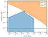 |
Fig. 1. Brunt-Väisälä (N; in blue), Lamb (for l = 2; S2; in orange), and tidal (ωt; in green) frequencies for a planetary companion orbiting an RGB star with MZAMS = 1 M⊙ at a distance of 1 AU. The colours mark the regions where the different types of waves can be excited (see the main text for details). |
2.2.3. Gravity waves
Gravity waves (g-waves) are waves that have buoyancy as their restoring force. These waves can be excited at frequencies lower than the Brunt-Väisälä frequency, N (in Hz; Aerts et al. 2010):
 (5)
(5)
where g0, p0, and ρ0 are the unperturbed gravitational acceleration (in cm/s2), pressure (in g/cm s2), and density (in g/cm3), respectively. Γ1 = (∂lnp0/∂lnρ0)S is the first adiabatic exponent, where S is the macroscopic entropy. This Brunt-Väisälä frequency is shown as a function of radius in Fig. 1 for a star with initial mass of 1 M⊙ during the AGB phase. Here the tidal frequency is also shown for a planet on a circular orbit at a distance of 1 AU. As can be seen, the tidal frequency is much lower than the maximal Brunt-Väisälä frequency (ωt ≪ Nmax), and therefore g-waves in the form of internal gravity waves (IGWs) can be excited by the tidal potential, and need to be taken into account when computing the dynamical tide and its dissipation.
Depending on the efficiency of the radiative damping, the waves are either damped before they can be reflected at the boundaries of the radiative zone, or they are reflected at the boundaries and travel back and forth through the radiative zone. In the former case, the waves are called progressive gravity waves; in the latter case, the reflecting interaction of the waves creates standing gravity modes. The two cases are separated by the critical frequency, νc, which is the frequency at which the radiative damping is strong enough to damp the waves with a factor e before they can be reflected at the boundaries of the radiative zone. νc (in Hz) can be expressed as (Alvan et al. 2015)
![Mathematical equation: $$ \begin{aligned} \nu _{\rm c} = [l(l+1)]^{\frac{3}{8}}\left(\left| \int _{r_{\rm in}}^{r_{\rm out}} K_{\mathrm{T} } \frac{N^3}{r_1^3} \mathrm{~d} r_1\right|\right)^{\frac{1}{4}}\ , \end{aligned} $$](/articles/aa/full_html/2024/10/aa49648-24/aa49648-24-eq9.gif) (6)
(6)
where KT is the thermal diffusivity (in cm2/s, calculated following Viallet et al. 2015). Frequencies lower than the critical frequency are progressive gravity waves, while frequencies higher than the critical frequency are gravity modes.
Here rin and rout are the inner and outer boundaries of the radiative zone assuming a three-layer structure (see Fig. 2). In the case there is only a radiative core and a convective envelope, rin = 0 and rout = rc. In the case there is a convective core and a radiative envelope, rin = rc and rout = R⋆. In the case of a three-layer structure (such as in MS F-type stars, or horizontal branch stars), one needs to be careful with this definition as waves starting at the inner boundary may interact with waves starting at the outer boundary, and may still create g-modes in the progressive wave regime.
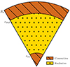 |
Fig. 2. Schematic representation of the radiative and convective shells in the case of the three-layer structure used in this study. Radii are not to scale for a real stellar structure (see the Kippenhahn diagrams, e.g. Fig. 5). |
When the amplitude of the g-waves become sufficiently large, the waves can start to feel non-linear effects known as wave breaking (Barker & Ogilvie 2010; Barker 2020). In this case an absorption barrier is created, such that the waves cannot be reflected, and the waves are absorbed. When this occurs the waves are not able to form standing modes, and our formalism still holds for frequency above the critical frequency.
The critical frequency in evolved stars is higher than the tidal frequency (see Sect. 4.1), and therefore the tidal potential will mostly excite progressive gravity waves in evolved stars.
2.3. Tidal dissipation
2.3.1. Equilibrium tide
The equilibrium tide is the tidal dissipation originating from the hydrostatic deformation of an object due to the gravitational potential of a companion (Zahn 1966, 1989). The equilibrium tide is dissipated through turbulent friction in convective layers. In order to calculate the dissipation of the equilibrium tide, the tidal displacement of the star needs to be calculated. To calculate this displacement, the non-wave-like component of the gravitational potential Φlnw needs to be obtained. This is done by solving the differential equation (e.g. Zahn 1966; Dhouib et al. 2024)
 (7)
(7)
for l = 2, where Ψl the tidal potential (in erg). Boundary conditions are chosen to ensure regularity at the centre and continuity at the surface (Ogilvie 2013; Dhouib et al. 2024):
 (8)
(8)
When the non-wave-like component of the gravitational potential is known, the tidal displacement (in cm, radial r and horizontal h components) can be calculated following (Zahn 1966; Remus et al. 2012; Dhouib et al. 2024) to ensure the equilibrium tide continuity at each radiative-convective boundary:
 (9)
(9)
Then, using these expressions, we computed the dissipation of the equilibrium tide following Barker (2020):
 (10)
(10)
with
 (11)
(11)
where l = 2 and νt(x) is the turbulent viscosity (in cm2/s) given by (Duguid et al. 2020)
![Mathematical equation: $$ \begin{aligned} \nu _t=V_{\mathrm{c} } l_{\mathrm{c} } F(\omega _t),\ F(\omega _t) = {\left\{ \begin{array}{ll} 5&|\omega _t|t_{\mathrm{c} } < 10^{-2} \\ \frac{1}{2}\left(|\omega _t| t_{\mathrm{c} }\right)^{-\frac{1}{2}}&|\omega _t| t_{\mathrm{c} } \in \left[10^{-2}, 5\right] \\ \frac{25}{\sqrt{20}}\left(|\omega _t| t_{\mathrm{c} }\right)^{-2}&|\omega _t| t_{\mathrm{c} }>5\ , \end{array}\right.} \end{aligned} $$](/articles/aa/full_html/2024/10/aa49648-24/aa49648-24-eq15.gif) (12)
(12)
with Vc the convective velocity (in cm/s), lc the mixing length (in cm), and tc the convective turnover time (in s).
2.3.2. Dynamical tide for progressive IGWs
In addition to the equilibrium tide is the dynamical tide, constituted here by progressive IGWs. These waves are excited (with their frequency the tidal frequency, ωt) and are dissipated through radiative damping (e.g. Zahn 1975; Goldreich & Nicholson 1989).
Assuming the three-layer structure (see Fig. 2), the tidal dissipation can be calculated for waves emerging from the convective core and the convective envelope (the derivation can be found in Appendix B, which in the limit of a low companion mass, i.e. a planet, is equal to the formula derived by Ahuir et al. 2021a):
![Mathematical equation: $$ \begin{aligned} \begin{aligned} {\text{ Im}}\left(k^2_2\right)_{\rm IGW}=&\frac{3^{-\frac{1}{3}} \Gamma ^2\left(\frac{1}{3}\right)}{2 \pi } [l(l+1)]^{-\frac{4}{3}} \omega _t^{\frac{8}{3}} \frac{a^6}{GM_2^2 R_{\star }^5} \\&\begin{aligned}\times \Bigg ( \rho _0\left(r_{\rm in}\right) r_{\rm in}&\left|\frac{d N^2}{\mathrm{~d} \ln r}\right|_{r_{\rm in}}^{-\frac{1}{3}} \mathcal{F} _{\rm {in}}^2\\&+\rho _0\left(r_{\rm out}\right) r_{\rm out}\left|\frac{d N^2}{\mathrm{~d} \ln r}\right|_{r_{\rm out}}^{-\frac{1}{3}} \mathcal{F} _{\rm {out}}^2 \Bigg )\ ,\end{aligned} \end{aligned} \end{aligned} $$](/articles/aa/full_html/2024/10/aa49648-24/aa49648-24-eq16.gif) (13)
(13)
with ℱout and ℱin being the tidal forcing (in cm2) at the inner and outer boundary of the radiative zone, and Γ the gamma function (Abramowitz & Stegun 1972). The tidal forcing term at the inner and outer boundary of the radiative zone can be expressed as (Ahuir et al. 2021a)
![Mathematical equation: $$ \begin{aligned} \begin{aligned} \mathcal{F} _{\mathrm{in}}&=\int _0^{r_{\rm in}}\left[\left(\frac{r^2 \varphi _T}{g_0}\right)^{\prime \prime }-\frac{l(l+1)}{r^2}\left(\frac{r^2 \varphi _T}{g_0}\right)\right] \frac{X_{1, \text{ in}}}{X_{1, \mathrm{in}}\left(r_{\mathrm{in}}\right)} d r \\ \mathcal{F} _{\mathrm{out}}&=\int _{r_{\mathrm{out}}}^{R_{\star }}\left[\left(\frac{r^2 \varphi _T}{g_0}\right)^{\prime \prime }-\frac{l(l+1)}{r^2}\left(\frac{r^2 \varphi _T}{g_0}\right)\right] \frac{X_{1, \mathrm{out}}}{X_{1, \mathrm{out}}\left(r_{\mathrm{out}}\right)} d r \end{aligned}\ , \end{aligned} $$](/articles/aa/full_html/2024/10/aa49648-24/aa49648-24-eq17.gif) (14)
(14)
where X1, out and X1, in are representations for the radial displacement originating from the inner and outer boundary of the radiative zone, and φT is defined in Eq. (2). The radial displacement can be calculated using the following differential equations and boundary conditions (Ahuir et al. 2021a):
 (15)
(15)
where the proportionality factor in the boundary conditions is cancelled out as X is always rescaled to the interaction region X/X(rint) in Eq. (14). The boundary conditions are calculated by assuming that  is small close to the centre of the star, and that
  is small close to the surface of the star in the case of the studied coplanar circular orbit of the companion for which l = m = 2.
3. Stellar evolution models
To study the different tidal dissipation mechanisms throughout a star’s lifetime, stellar evolutionary models are necessary. In this study we used the Modules for Experiments in Stellar Astrophysics (MESA) code (Paxton et al. 2011, 2013, 2015, 2018, 2019; Jermyn et al. 2023) to calculate these stellar evolutionary models. Models were computed for zero age main sequence (ZAMS) stars with masses between 1 and 4 M⊙ at solar metallicity (Z = 0.0134; Asplund et al. 2009). The Hertzsprung-Russell (HR) diagram for these stars is shown in Fig. 32. These masses are chosen to allow the study of a range of stellar evolutionary effects such as the difference between a convective or radiative envelope during the MS and the difference between a helium flash or gradual helium burning. The models are computed from the PMS up to the white dwarf (WD) stage. The models are terminated when the WD is cooled down sufficiently to have a luminosity of L = 10−1 L⊙.
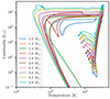 |
Fig. 3. Hertzsprung-Russell diagram of the stellar evolutionary models studied here. The models start in the PMS and are evolved up to the WD phase. Different colours indicate a different ZAMS mass, as indicated in the box in the left-bottom corner. |
To simulate convection, the mixing length theory (MLT) was used following the prescription of Henyey et al. (1965). In this prescription, αMLT is the mixing length parameter, which is calibrated by Cinquegrana & Joyce (2022) to reproduce the solar radius and luminosity at the solar age, resulting in αMLT = 1.931. As evolved stars have relative low temperatures, a dedicated low-temperature molecular opacity table (ÆSOPUS; Marigo & Aringer 2009) is used. For the atmosphere, a grey temperature-opacity (T − τ, where τ is the optical depth) relation is assumed, based on the Eddington relation (Paxton et al. 2011).
The mass-loss rate is calculated using the Reimers prescription (Reimers 1975) during the RGB phase, with a scaling factor of ηReimers = 0.477 (McDonald & Zijlstra 2015). During the AGB phase, the Blöcker prescription (Blöcker 1995) is used with a scaling factor of ηBlöcker = 0.05 for masses below 2 M⊙ and ηBlöcker = 0.1 for masses above 2 M⊙ (Madappatt et al. 2016).
Stars undergo internal mixing, which is described by convective mixing in the convective zone. Radiative layers are also the seat of mild mixing and transport mechanisms (see e.g. Zahn 1992; Mathis 2013; Aerts et al. 2019). To have a simple description of the mixing in the radiative zone, we assumed a constant uniform mixing coefficient Dmin = 10 cm2 s−1 throughout the radiative layers. Multiple values were tested for Dmin, and the resulting tidal dissipation was found to be insensitive to the exact value of Dmin. This value was chosen to improve numerical stability within the MESA simulations.
4. Tidal dissipation along stellar evolution
During the evolution of the star, the strength of tidal dissipation varies due to the changes in internal structure and rotation (e.g. Mathis 2015; Gallet et al. 2017; Bolmont et al. 2017; Barker 2020; Ahuir et al. 2021a. In this section, we investigate the tidal dissipation along the stellar evolution, focusing specifically on advanced stages from the RGB to the WD stages. To verify our results, we benchmarked them with the values of the dissipation of the equilibrium and dynamical tides found in Ahuir et al. (2021a), who computed of the equilibrium and dynamical tide dissipation up to the RGB phase. The comparison was done for the 1, 1.2 and 1.4 M⊙ stars in Appendix C. We find good agreement between our results and the results of Ahuir et al. (2021a). Before going into detail on the tidal dissipation, we validate our formalism by examining the critical period as a function of stellar mass.
4.1. Critical period
The critical period (Pc = 1/νc; Eq. (6)) as a function of stellar age is shown in Fig. 4 for all stellar evolutionary models used in this study3. During the PMS, the critical period is high (higher than a few days), and decreases until the MS starts. During the MS, the critical period remains approximately constant, and decreases when the RGB phase starts. Afterwards, the critical period remains low (lower than 0.1 day). This means that our formalism is valid for stars along the evolved phases.
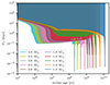 |
Fig. 4. Critical period, Pc = 1/νc, for different stellar masses. The different colours represents the same model as in Fig. 3. The filled regions indicate where the g-waves are excited as progressive IGWs. |
The critical period also depends on the initial mass of the star. For lower-mass stars (e.g. the 1 M⊙ model), the critical period is approximately 3 days during the MS, while for higher-mass stars (e.g. the 4 M⊙ model), the critical period is approximately 0.1 days during the MS. Therefore, it is possible for short-period companions (with periods of the order of 1 day) around the lower-mass stars (below or equal to 1.2 M⊙) in the MS to excite g-modes in the radiative layer instead of progressive IGWs. The tidal dissipation of these g-modes is likely to be more effective than the tidal dissipation estimated in this study, since standing modes might experience enhanced dissipation efficiency, potentially amplified through resonance locking (e.g. Witte & Savonije 2002; Fuller 2017).
In principle, wave breaking can also dissipate the waves, but as the critical period is short during the evolved phases, the waves will already be damped before they can break. This is not the case for the lower-mass stars in the MS phase and possibly during the sub-giant phase (e.g. Weinberg et al. 2017), where the critical period is higher, and the waves can break. For an investigation of wave breaking during the MS and the sub-giant phase, we refer the reader to Barker (2020) and Ahuir et al. (2021a) in their Appendix D.
4.2. Earth around the Sun
4.2.1. Internal structure of a 1 M⊙ star
Tidal dissipation depends strongly on the internal structure of the star. Fig. 5 shows the Kippenhahn of a MZAMS = 1 M⊙ star. Here the stellar age is visualised as the time until the end of the simulation, that is, the time until the WD is cool enough to produce a luminosity of L = 10−1 L⊙. When plotting this time in logarithmic scale, the evolved phases can be shown in a single plot. The different evolutionary phases are indicated in Fig. 5. During the MS, the radius increases gradually, where the star has a convective envelope and a radiative core. After the MS, the star starts to expand rapidly, and the convective envelope grows. During the RGB phase, the star has a convective envelope and a radiative interior. When the star reaches the tip of the RGB, it contracts during the helium flash (brief thermal runaway nuclear burning of helium caused by the growth of the degenerate core), where the radius of the stars stays relatively constant during the horizontal branch (HB). During this phase, the star has a convective core, creating a three-layer structure. After the HB, the star expands again, and the star has a convective envelope and a radiative core in the AGB phase. When the star reaches the tip of the AGB, the star contracts again, and the star leaves the AGB track to cool down as a WD. During the WD phase, the star has a radiative interior.
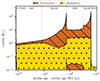 |
Fig. 5. Kippenhahn diagram for a MZAMS = 1 M⊙ star. The brown hatched region represents convective layers, and the yellow dotted region represents radiative layers. The upper layer represents the radius of the star. Stellar evolutionary phases (PMS to WD) are indicated. |
4.2.2. Tidal dissipation
We considered a planet with an orbit of 1 yr and the mass of the Earth (e.g. the Earth) that is rotating around such a star with an initial mass of 1 M⊙ (e.g. the Sun). For simplicity, the orbit was assumed to remain at a period of 1 yr. In Fig. 6, we show the evolution of the imaginary part of the Love number both for the equilibrium and dynamical tides as a function of time. Looking at the equilibrium tide in the figure, the Love number follows the trend of the radius quite well. When the radius increases, the Love number increases, and vice versa. This is due to the fact that for stars with a larger radius, the local gravity is weaker, and therefore the star is more easily deformed by the tidal potential. This results in larger values of ξr and ξh, and a larger integral in Eq. (10). This is compensated by the dependance of R⋆−(2l + 1) (including the R⋆l dependence of φT(R⋆)) from the denominator in the equation. Inside the integral the dependance on R⋆ is a bit more complicated. Starting with ξr and ξh, which are dependant on R⋆4 (R⋆2 from the tidal potential, and R⋆2 from the reduction of the local gravity; see Eq. 9), which appears squared divided by the radius inside Dl (see Eq. 11). This results in a R⋆6 dependance of Dl, and a R⋆8 dependance inside the integral (from the r2 inside the integral). The integral is thus dependant on R⋆9 (due to the integration), resulting in a R⋆4 dependance of the equilibrium tide dissipation (in agreement with Remus et al. 2012).
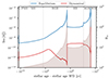 |
Fig. 6. Complex part of the Love number (Im(k22)) for both equilibrium (blue) and dynamical (red) tides (left axis) and stellar radius (brown; right axis) as a function of stellar age for a MZAMS = 1 M⊙ star with a 1 MEarth companion at 1 AU. Stellar evolutionary phases (PMS to WD) are indicated. |
This is not the case for the dynamical tide. To explain the complex behaviour of its dissipation, the different components appearing in the dissipation of the dynamical tide (Eq. 13) are shown as a function of stellar age in Fig. 7. The change in radius of the radiative-convective boundary, change in stellar mass and change in the derivative of the Brunt-Väisälä frequency are small compared to the changes in the tidal forcing and local density at the boundary. This is due to the low power of the Brunt-Väisälä frequency and the boundary radius, as well as the small change in the stellar mass. The dissipation is proportional to R⋆−5, and thus the dynamical tide dissipation responds inversely to an increase in radius4. This effect is counteracted by the tidal forcing, ℱ, which depends on φT, which in turn scales as R⋆2. When multiplying their contributions, a complex pattern appears (as can be seen in red in Fig. 7). First this multiplication coefficient (ℱ2/R⋆5) increases, as the star increases while the size of the convective envelope remains approximately constant. When the convective envelope starts to becomes thicker at the start of the RGB, the tidal forcing grows more slowly than the stellar radius increases, as X(r)/Xout decreases as Xout increases for larger sizes of the convective envelope, and therefore the multiplication coefficient decreases. At the same time the local density at the boundary layer decreases as well, due to the large extend (and thus low density) of the envelope. This combination results in a dissipation of the dynamical tide that first increase during the sub-giant phase and at the start of the RGB (in agreement with Ahuir et al. 2021a) and then decrease during the RGB (see Fig. 6). When the helium flash occurs and the star contracts, the extent of the radiative interior increases again, and therefore the tidal forcing increases. For that reason, the dynamical tide dissipation is stronger during the HB compared to the dissipation during the RGB. Additionally, the star has a small convective core in this phase, and there is a contribution from the inner boundary of the radiative zone to the tidal dissipation, but this component is negligible compared to the contribution from the outer boundary. During the HB, the internal structure remains approximately constant, and therefore the tidal dissipation remains approximately constant. When the star starts to expand during the AGB, the size of the radiative core remains approximately constant, and therefore the multiplication coefficient remains approximately constant as well. However, as the stellar radius grows, and therefore the density at the boundary layer decreases, the dynamical tide dissipation decreases in strength. During the WD phase, the star is fully radiative. In this case tidally forced (travelling) waves can still be excited, but not at a radiative-convective boundary, and thus our formalism no longer applies. The dynamical tide can now excite standing gravity modes (Fuller & Lai 2011, 2012, 2013, 2014) for stellar companions or f-modes (Veras & Fuller 2019) for planetary companions. These dynamical tides are not calculated in this study.
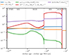 |
Fig. 7. Different components appearing in the dissipation of the dynamical tide (Eq. (13)) as a function of stellar age. The change in radius of the radiative-convective boundary is represented in blue, the change in stellar mass in orange, the change in local density at the boundary in green, the change in tidal forcing compared to changes in the stellar radius in red, and change in the derivative of the Brunt-Väisälä frequency in purple. Stellar evolutionary phases (PMS to WD) are indicated. |
Overall the tidal dissipation of the equilibrium tide is dominant compared to the dissipation of the dynamical tide at this orbital period. But as they have different dependencies this will change for different orbital periods and different primary and secondary masses, which is shown in the next sections.
4.3. Dependence of tidal dissipation on the orbital period
The strength of the equilibrium and dynamical tides are dependent on the orbital distance. For the equilibrium tide dissipation this is captured in the linear dependence on ωt, but there is also a complex dependence of the turbulent viscosity on ωt (see Eq. 12). For the dynamical tide dissipation there is a dependence in ωt, Ωo, the tidal forcing, and the boundary conditions of X. This results in a complex dependence on the orbital period, which is investigated for a 1 MJup planet around a 1 M⊙ star.
4.3.1. Equilibrium tide
The dissipation of the equilibrium tide as a function of stellar age and orbital period is shown in Fig. 8. When a companion is too close to the star, the companion will be destroyed by tidal forces. This is represented by the Roche limit, which is shown for a M = 1 MJup, R = 1 RJup planet in Fig. 8 in purple (for the details of its calculation, we refer to Benbakoura et al. 2019). When the Roche limit is located inside the star, it is no longer a relevant parameter. In this case a planet might plunge inside the star and reach deep layers before being completely destroyed (Lau et al. 2022). Here it can be seen that by increasing the orbital period, the equilibrium tide dissipation increases until a maximum is reached, after which the equilibrium tide dissipation becomes weaker again. The reason is that for low orbital periods, the tidal frequency is sufficiently high such that in the dominant region (the region where most of the dissipation occurs) the turbulent viscosity is proportional to the inverse square of the tidal frequency. Because there is an additional linear dependence of the tidal frequency on the Love number of the equilibrium tide, the dissipation of the equilibrium tide is proportional to the inverse of the tidal frequency, and hence will increase with increasing orbital period. However, when the orbital period is sufficiently high, the tidal frequency times the convective time tc becomes high enough (see Eq. (12)) such that the turbulent viscosity is proportional to the inverse square root of the tidal frequency, and thus the dissipation of the equilibrium tide is proportional to the square root of the tidal frequency. Therefore, by increasing the orbital period further, the equilibrium tide dissipation will decrease. The final regime of Eq. (12), where the turbulent viscosity is independent of the tidal frequency, is not reached in this study, as the orbital periods are not high enough.
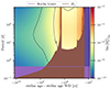 |
Fig. 8. Complex part of the Love number for the equilibrium tide (Im(k22)eq) as a function of the orbital period and stellar age for a MZAMS = 1 M⊙ star. R⋆ (in brown) represents the orbital period on which a planet orbits at the surface of the star, and the Roche limit is given in purple. Changes in the stellar evolutionary phase are indicated with ticks on the upper axis. |
4.3.2. Dynamical tide
The dynamical tide dissipation as a function of stellar age and orbital period is shown in Fig. 9. Here it can be seen that by increasing the orbital period, the dynamical tide dissipation strictly decreases. Looking at Eq. (13), there is a dependence on ωt, Ωo, the tidal forcing, and the boundary conditions of X. The tidal forcing is proportional to the square of the orbital period (as there is φT, which has a dependence of a−3 ∝ Ωo2). Hence, this cancels out the direct dependence on the orbital frequency in the equation. The dependence in the boundary condition of X on the orbital period (again due to φT) remains small, and only has a small effect at low orbital periods. The dependence on ωt8/3 is the dominant factor, and thus the dynamical tide dissipation is proportional to  . At the end of the star’s evolution, when the star is a WD and the star is fully radiative, the dynamical tide is not calculated as our formalism does not hold. Therefore, this region is left blank in Fig. 9. In this region, the dynamical tide can be composed of standing g- and f-modes (Fuller & Lai 2011, 2012, 2013, 2014; Veras & Fuller 2019) and thus its dissipation will have a different dependence on the orbital period.
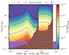 |
Fig. 9. Complex part of the Love number for the dynamical tide (Im(k22)IGW) as a function of orbital period and stellar age for a MZAMS = 1 M⊙ star. The critical period, Pc, above which companions excite progressive IGWs, is shown in orange. R⋆ (in brown) represents the orbital period on which a planet orbits at the surface of the star, and the Roche limit is given in purple. Changes in the stellar evolutionary phase are indicated with ticks on the upper axis. |
4.3.3. Relative strengths
Since the strengths of the equilibrium and dynamical tide dissipation have a different dependence on stellar age and orbital period, the dissipation of the equilibrium tide will be dominant in some regions of the parameter space, while in other regions, the dissipation of the dynamical tide will be more important. This can be seen in Fig. 10, where their ratio is shown. During the MS, the dynamical tide dissipation is dominant (a factor of 10 higher than the equilibrium tide dissipation) for orbits shorter than a 10 days in agreement with previous work (Ahuir et al. 2021a). There is a gradual change until orbital periods longer than 50 days where the equilibrium tide dissipation dominates. When the star enters the RGB, the equilibrium tide dissipation increases, while the dynamical tide dissipation decreases (see Sect. 4.2.2), resulting in the equilibrium tide dissipation becoming dominant for shorter orbital periods, and dominating completely when the star is sufficiently large. When the star contracts and becomes a HB star, the dynamical tide dissipation becomes stronger, remaining relevant again for orbits up to 30 days. When the star enters the AGB, the equilibrium tide dissipation becomes dominant again, similar to the RGB phase. When the star contracts to become a WD, the star becomes fully radiative and our formalism can no longer be applied. Then, the dissipation of the equilibrium tide dominates. However, in such a configuration, tidal g- and f-modes can be excited and their dissipation may dominate that of the equilibrium tide.
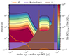 |
Fig. 10. Ratio of the complex parts of the Love number for the dynamical to equilibrium tide (Im(k22)IGW/Im(k22)eq) as a function of the orbital period and stellar age for a MZAMS = 1 M⊙ star. The critical period, Pc, above which companions excite progressive IGWs, is shown in orange. R⋆ (in brown) represents the orbital period on which a planet orbits at the surface of the star, and the Roche limit is given in purple. Changes in the stellar evolutionary phase are indicated with ticks on the upper axis. |
4.4. Dependence of the tidal dissipation on the secondary mass
The dependence of the tidal dissipation on the secondary mass is complex, and is dependent on whether we assume the orbital period and orbital distance to vary as a function of this parameter or not. Let us first assume that both the orbital period and distance are constant, a good approximation when only varying companion mass, which is negligible compared to the mass of the primary star as in the case of the planet. Then, the relation between the semi-major axis and the orbital period has only a weak dependence on the secondary mass. In this situation, there is a dependence on the secondary mass via φT and Dl, with φT being proportional to M2 and Dl being proportional to M22. Therefore, the equilibrium tide dissipation given in Eq. (10) is independent of the mass of the companion. For the dynamical tide dissipation (Eq. 13), there is direct dependence on the secondary mass as well as on ℱ, which contains φT. The direct dependence on the mass of the companion cancels out again. This is expected as the Love number is defined as the ratio between the perturbation of the primary’s gravitational potential induced by the presence of the companion and the tidal potential, evaluated at the stellar surface, and the direct dependence of the secondary mass in both the numerator and denominator is the same, resulting in a constant Love number as a function of M2.
However, when the companion becomes more massive, the relation between the orbital period and the orbital distance (a3/P2 = G(M1 + M2)/4π2) becomes dependent on the secondary mass. Let us now consider the situation where the orbital period is fixed. Then, the change in the semi-major axis is proportional to ![Mathematical equation: $ \sqrt[3]{M_1 + M_2} $](/articles/aa/full_html/2024/10/aa49648-24/aa49648-24-eq22.gif) for this fixed orbital period. Given the fact that the tidal forcing ℱ is inversely dependent on the semi-major axis cubed ℱ ∝ M2/a3 (due to its dependance on φT; see Eq. 2), the tidal forcing changes with a factor ℱ ∝ M1M2/(M1 + M2) compared to a companion with a small (negligible) mass. The dynamical tidal dissipation, however, also has a direct dependence on the semi-major axis (as well as on M2). This dependence is exactly the same as the tidal forcing, and thus the dynamical tide dissipation will be constant with respect to changes in the secondary mass when the orbital period is fixed. The same is true for the equilibrium tide dissipation, as the dependence of the semi-major axis is the same in the tidal displacement and the tidal potential. This confirms that tidal dissipation is an intrinsic property of a celestial body, which does not depend on the property of the secondary (excepting through the tidal frequency).
for this fixed orbital period. Given the fact that the tidal forcing ℱ is inversely dependent on the semi-major axis cubed ℱ ∝ M2/a3 (due to its dependance on φT; see Eq. 2), the tidal forcing changes with a factor ℱ ∝ M1M2/(M1 + M2) compared to a companion with a small (negligible) mass. The dynamical tidal dissipation, however, also has a direct dependence on the semi-major axis (as well as on M2). This dependence is exactly the same as the tidal forcing, and thus the dynamical tide dissipation will be constant with respect to changes in the secondary mass when the orbital period is fixed. The same is true for the equilibrium tide dissipation, as the dependence of the semi-major axis is the same in the tidal displacement and the tidal potential. This confirms that tidal dissipation is an intrinsic property of a celestial body, which does not depend on the property of the secondary (excepting through the tidal frequency).
On the other hand when fixing the semi-major axis a, but allowing the orbital period to vary by changing the secondary mass, the orbital frequency and thus the tidal frequency will change, with the orbital period being proportional to  . Since the semi-major axis remains constant in this situation, the tidal forcing becomes linear as a function of M2 (cancelled out by the direct dependance of Im(k22)IGW on M2). Therefore, the dynamical tide dissipation will be proportional to ωt8/3 and thus proportional to
  . For higher-mass companions, the dynamical tide dissipation will become stronger with a factor ((M1 + M2)/M1)4/3 (Im(k22)IGW ∝ ((M1 + M2)/M1)4/3) compared to a companion with a small (negligible) mass. In this case the equilibrium tide dissipation will be affected as well. Due to the complex dependence of the turbulent viscosity on the tidal frequency, there is no direct proportionality constant that can be applied. However, one can still read Fig. 8 the same way, only for an orbital period that changes proportional to
  . Depending on the orbital separation, and thus the regime of the turbulent viscosity, the equilibrium tide can become stronger or weaker (see Sect. 4.3.1).
4.5. Dependence of the tidal dissipation on the primary mass
The strength of the dissipation of the equilibrium and dynamical tides are dependent on the mass of the primary star and the evolutionary stage. In this section we investigate the dependence of the tidal dissipation on the primary stellar mass and age using the grid of stellar models with initial masses between 1 and 4 M⊙. The Kippenhahn diagram, together with the complex part of the Love number for both the equilibrium and dynamical tides as well as the ratio of their dissipation as a function of stellar age and orbital period, is shown in Figs. 11, 12, and 13, as well as in Appendix D5.
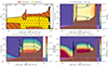 |
Fig. 11. Internal structure and tidal dissipation evolution for a MZAMS = 2 M⊙ star. Top left: Kippenhahn diagram. The brown hatched regions represent convective layers, and the yellow dotted region represents radiative layers. Stellar evolutionary phases (PMS to WD) are indicated. Top right, bottom left, and bottom right: Complex part of the Love number for the equilibrium tide (Im(k22)eq), the dynamical tide (Im(k22)IGW), and the ratio of the dissipations of the dynamical tide to the dissipation of the equilibrium tide (Im(k22)IGW/Im(k22)eq), respectively, as a function of stellar age and orbital period. The Roche limit is shown in purple, the critical period (1/νc; see Eq. 6) in orange, and the period at which a planet orbits at the stellar radius in brown. Changes in the stellar evolutionary phase are indicated with ticks on the upper axis. |
4.5.1. Changes during the MS and RGB
When stars start their evolution with different initial masses, the internal structure on the MS changes. Lower-mass stars have a convective envelope and a radiative interior (like the 1 M⊙ star). Higher-mass stars have a convective core and a radiative envelope, like for instance a 2 M⊙ star (see Fig. 11). In between there is a transition zone where there is a true three-layer structure, with a convective core, a radiative envelope and a convective envelope. This transition zone is dependent on the stellar evolution parameters used, where in our models the three-layer structure is apparent in the 1.2 and 1.4 M⊙ models (see Figs. D.1 and D.2). For higher-mass stars with a radiative envelope (the star still has a tiny convective envelope at the surface of the star), the equilibrium tide dissipation is drastically reduced, as well as the dynamical tide dissipation arising from the tiny convective envelope. At this point, the dynamical tide arising from the convective core propagating in the radiative envelope becomes dominant for short orbital periods (in agreement with Zahn 1975, 1977; Goldreich & Nicholson 1989). This dominance over the equilibrium tide dissipation is less pronounced compared to the 1 M⊙ star. This dynamical tide arising from the convective core decreases during the MS, as the size of the convective core is reduced during this phase, while at the same time the radius increases. When these stars evolve into RGB stars, the convective envelope reappears, and the equilibrium tide dissipation from this region and the dynamical tide excited at the boundary between the radiative core and the convective envelope become dominant again. This results in a sudden increase in the ratio of the dissipation of the dynamical to equilibrium tide, and afterwards it decreases similarly to the 1 M⊙ star.
4.5.2. Changes during the HB and AGB
When stars evolve from the RGB into the HB, they will go through a helium flash for low-mass stars (up to MZAMS= 2 M⊙), while for intermediate-mass stars (above 2 M⊙) the burning of helium starts gradually. For low-mass stars, this results in a sudden contraction of the star, and a sudden increase in the ratio of the dissipation of the dynamical to equilibrium tide (see Sect. 4.2.2). For intermediate-mass stars, the star will slowly contract, resulting in a slow increase in this ratio.
The length of the RGB phase is also dependent on the star’s initial mass. For lower-mass stars, the RGB phase is more pronounced compared to higher-mass stars. For lower-mass stars (with masses lower than 2 M⊙ where the star goes through a helium flash), the maximal radius reached during the RGB is roughly the same with increasing stellar mass. Due to the increase in stellar mass, the period a companion has when it would orbit at the radius of the star at the tip of the RGB will be lower. For higher-mass stars (with masses higher than 2 M⊙ with gradual helium ignition) the maximal radius reached during the RGB increases with increasing stellar mass, but the radius remains small compared to the stars with a helium flash. At the same time, because of the increase in mass, the dynamical tide dissipation also increases (see Eq. (13)), making the dynamical tide more important during the HB phase for these stars. Because of these two effects, the dynamical tide dissipation is important for companions at larger orbital distances than the primary’s radius reached at the tip of the RGB (see e.g. Figs. 11 and 12).
When increasing further in mass to the most massive model of 4 M⊙ (see Fig. 13), the convective envelope goes through a similar evolution when the star is contracting gradually after the start of helium burning. Hence, the dissipation from both the equilibrium and dynamical tides increases, with similar relative strengths as for the 3.5 M⊙ model (Fig. 12). When the star is fully contracted throughout the HB, the convective envelope is smaller for the 4 M⊙ model, reducing both the equilibrium and dynamical tide dissipation during this phase, where the dynamical tide dissipation is affected the most, reducing its relative importance. This effect is similar to the shift of convective to radiative envelope during the MS for 1 to 1.4 M⊙ models.
During the AGB phase, the trends of the equilibrium and dynamical tidal dissipation remain similar for all masses. At the start of the AGB phase, the ratio of the dissipation of the dynamical to equilibrium tide starts to decrease due to the increase in the primary’s radius, similar to the RGB phase. As the relative importance of the dynamical tide dissipation increases with increasing mass during the HB phase, the relative importance also increases at the start of the AGB phase, but its importance becomes negligible early in the AGB phase. In the late stages of the AGB phase, the star will undergo thermal pulses (a periodic instability marked by the sudden ignition of helium in a thin shell around the carbon-oxygen core that leads to temporary structural and luminosity changes). This will alter the internal structure of the star, and therefore the tidal dissipation. During a thermal pulse the star will undergo helium shell flashes, temporarily increasing its stellar radius, to afterwards go back to its original state. Therefore, the equilibrium tide dissipation will increase during such a pulse. The dynamical tide dissipation will change as well, but throughout all the models the dynamical tide dissipation is negligible compared to the equilibrium tide dissipation during these thermal pulses.
5. Conclusion
This study investigated the dissipation of the equilibrium and dynamical tides from progressive IGWs (where the dynamical tide from inertial waves is estimated to be negligible) throughout the entire evolution of stars, with a strong focus on the evolved phases. A grid of stellar evolutionary models was created with initial masses between 1 and 4 M⊙. This allowed the investigation of different stellar evolutionary effects on the tidal dissipation, such as the difference between a convective and radiative envelope during the MS, or the difference between a helium flash and gradual helium burning. Using these models, we investigated the dependence on the orbital period, the mass of the primary star, and the mass of the companion. For stars with a sufficiently low primary mass such that the star has a radiative core and a convective envelope in the MS, the dynamical tide dissipation is dominant for orbital periods shorter than 10 days, in agreement with Terquem et al. (1998), Goodman & Dickson (1998), Barker & Ogilvie (2010), and Ahuir et al. (2021a), while the equilibrium tide dissipation dominates for orbital periods longer than 50 days. For stars with a sufficiently high initial mass that the star has a radiative envelope and a convective core in the MS, tidal dissipation is dominated by the dynamical tide originating from the core for short orbital periods, in agreement with Zahn (1975). For longer orbital periods, the equilibrium tide dissipation dominates. At the start of the RGB, the dynamical tide dissipation first increases due to the increase in the spatial extent of the convective envelope that leads to an increase in the tidal forcing. For stars that already have a convective envelope during the MS, this is a gradual increase, while for stars that have a radiative envelope during the MS, the increase is instantaneous. During the RGB, the importance of the dynamical tide dissipation decreases as the radius of the star increases. At the start of the HB, the dynamical tide dissipation becomes more important again, as the radius of the star decreases either instantaneously in a helium flash or steadily when helium burning starts gradually. During the HB, the importance of the dynamical tide dissipation increases with increasing stellar mass. For sufficiently high masses (4 M⊙), the importance of the dynamical tide dissipation decreases instead of increasing as the size of the convective envelope shrinks. During the AGB, the equilibrium tide dissipation becomes dominant again due to the increase in stellar radius, similar to the RGB phase. During the WD phase, as the star is fully radiative, our formalism for the dynamical tide does not apply. However, this might be different when the dynamical tidal dissipation from standing g- and f-modes (Fuller & Lai 2011, 2012, 2013, 2014; Veras & Fuller 2019) is taken into account.
In a next step, these outcomes can be included when calculating the rate of change of the orbital distance of planetary and stellar companions along stellar evolution. The numerical model of a coplanar circular star-planet system called ESPEM (Benbakoura et al. 2019; Ahuir et al. 2021b) can be used to study the orbital evolution of a star-planet or star-star system. This model includes the tidal dissipation of the equilibrium tide dissipation as well as the dynamical tide arising from inertial waves propagating in convective envelopes. This code will be improved by including the dissipation of the dynamical tide arising from progressive IGWs (similar to Lazovik 2021, 2023), necessary for systems containing an evolved star. Furthermore, the rotation of the primary star is reduced due to magnetic breaking in ESPEM (Benbakoura et al. 2019; Ahuir et al. 2021b). In evolved stars, the magnetic breaking becomes negligible compared to the torque arising from the strong mass loss during this phase, which is not included in ESPEM as of now. It can be included by introducing a mass-losing outer shell (Madappatt et al. 2016), which depends on the current mass-loss rate of the star. The mass-loss rate of AGB stars is dependent on the presence of a companion, but ongoing work is still determining by how much (Decin et al. 2020; Aydi & Mohamed 2022). This will allow the study of the orbital distance evolution of star-planet and star-star systems around evolved stars and the resulting companion orbital distance and occurrence rate, as has been done for solar-like stars during the MS in García et al. (2023).
Furthermore, the orbital evolution of star-planet systems around evolved stars can be studied by taking the last breakthrough obtained through asteroseismology into account: asteroseismology is now revealing the presence of potentially strong magnetic fields in the core of red giants (Li et al. 2022, 2023; Deheuvels et al. 2023). Such strong magnetic fields can deeply modify the propagation of mixed modes, which behave as gravity modes in the core of red giants (e.g. Fuller et al. 2015; Bugnet et al. 2021; Mathis et al. 2021; Li et al. 2022; Mathis & Bugnet 2023; Rui & Fuller 2023; Rui et al. 2024) and can potentially be excited by tides. Determining the effect of such a potential modification of the propagation and dissipation of such tidal modes still requires a dedicated investigation as it could potentially alter the dynamics of planetary systems around these magnetic stars.
Calculated using the Extrasolar Planet Encyclopedia https://exoplanet.eu/, for planets with a R⋆ > 3 R⊙ star.
The inlist used to compute the stellar evolutionary models can be found both in Appendix E and on Zenodo: https://doi.org/10.5281/zenodo.11519523
The critical periods in this study are lower by a factor of 2π compared to Ahuir et al. (2021a) due to a unit conversion from s/rad to s.
Note that although the Love number is dependent on R⋆−5, when calculating the change in the semi-major axis of the orbit throughout time there is an additional factor of R⋆5 that cancels out this direct dependence on the stellar radius.
The Love numbers for these evolutionary models can be found on Zenodo: https://doi.org/10.5281/zenodo.11519523
Acknowledgments
The authors would like to thank Matthias Fabry, Hannah Brinkman, Timothy Van Reeth, and Pablo Marchant for their help and support in setting up the MESA stellar evolution models as well as Clément Baruteau for the useful discussions. The authors would also like to thank the anonymous referee for their constructive comments which helped to improve the quality of the paper. M. Esseldeurs, S. Mathis and L. Decin acknowledge support from the FWO grant G0B3823N. M. Esseldeurs and L. Decin acknowledge support from the FWO grant G099720N, the KU Leuven C1 excellence grant MAESTRO C16/17/007 and the KU Leuven IDN grant ESCHER IDN/19/028. S. Mathis acknowledges support from the PLATO CNES grant at CEA/DAp, from the Programme National de Planétologie (PNP-CNRS/INSU) and from the European Research Council through HORIZON ERC SyG Grant 4D-STAR 101071505. While partially funded by the European Union, views and opinions expressed are however those of the author only and do not necessarily reflect those of the European Union or the European Research Council. Neither the European Union nor the granting authority can be held responsible for them.
References
- Abramowitz, M., & Stegun, I. A. 1972, Handbook of Mathematical Functions [Google Scholar]
- Aerts, C., Christensen-Dalsgaard, J., & Kurtz, D. W. 2010, Asteroseismology (Springer Science+Business Media B.V.) [Google Scholar]
- Aerts, C., Mathis, S., & Rogers, T. M. 2019, ARA&A, 57, 35 [Google Scholar]
- Ahuir, J., Mathis, S., & Amard, L. 2021a, A&A, 651, A3 [NASA ADS] [CrossRef] [EDP Sciences] [Google Scholar]
- Ahuir, J., Strugarek, A., Brun, A. S., & Mathis, S. 2021b, A&A, 650, A126 [NASA ADS] [CrossRef] [EDP Sciences] [Google Scholar]
- Alvan, L., Strugarek, A., Brun, A. S., Mathis, S., & Garcia, R. A. 2015, A&A, 581, A112 [NASA ADS] [CrossRef] [EDP Sciences] [Google Scholar]
- Amard, L., Palacios, A., Charbonnel, C., Gallet, F., & Bouvier, J. 2016, A&A, 587, A105 [NASA ADS] [CrossRef] [EDP Sciences] [Google Scholar]
- Asplund, M., Grevesse, N., Sauval, A. J., & Scott, P. 2009, ARA&A, 47, 481 [NASA ADS] [CrossRef] [Google Scholar]
- Auclair Desrotour, P., Mathis, S., & Le Poncin-Lafitte, C. 2015, A&A, 581, A118 [NASA ADS] [CrossRef] [EDP Sciences] [Google Scholar]
- Aydi, E., & Mohamed, S. 2022, MNRAS, 513, 4405 [NASA ADS] [CrossRef] [Google Scholar]
- Barker, A. J. 2020, MNRAS, 498, 2270 [Google Scholar]
- Barker, A. J., & Ogilvie, G. I. 2010, MNRAS, 404, 1849 [NASA ADS] [Google Scholar]
- Beck, P. G., Mathis, S., Gallet, F., et al. 2018, MNRAS, 479, L123 [Google Scholar]
- Beck, P. G., Mathur, S., Hambleton, K., et al. 2022, A&A, 667, A31 [NASA ADS] [CrossRef] [EDP Sciences] [Google Scholar]
- Beck, P. G., Grossmann, D. H., Steinwender, L., et al. 2024, A&A, 682, A7 [NASA ADS] [CrossRef] [EDP Sciences] [Google Scholar]
- Benbakoura, M., Réville, V., Brun, A. S., Le Poncin-Lafitte, C., & Mathis, S. 2019, A&A, 621, A124 [NASA ADS] [CrossRef] [EDP Sciences] [Google Scholar]
- Blöcker, T. 1995, A&A, 297, 727 [NASA ADS] [Google Scholar]
- Bolmont, E., & Mathis, S. 2016, Celest. Mech. Dyn. Astron., 126, 275 [Google Scholar]
- Bolmont, E., Gallet, F., Mathis, S., et al. 2017, A&A, 604, A113 [NASA ADS] [CrossRef] [EDP Sciences] [Google Scholar]
- Bugnet, L., Prat, V., Mathis, S., et al. 2021, A&A, 650, A53 [NASA ADS] [CrossRef] [EDP Sciences] [Google Scholar]
- Ceillier, T., Tayar, J., Mathur, S., et al. 2017, A&A, 605, A111 [NASA ADS] [CrossRef] [EDP Sciences] [Google Scholar]
- Cinquegrana, G. C., & Joyce, M. 2022, Res. Notes Am. Astron. Soc., 6, 77 [Google Scholar]
- Decin, L., Montargès, M., Richards, A. M. S., et al. 2020, Science, 369, 1497 [Google Scholar]
- Deheuvels, S., Li, G., Ballot, J., & Lignières, F. 2023, A&A, 670, L16 [NASA ADS] [CrossRef] [EDP Sciences] [Google Scholar]
- Dhouib, H., Baruteau, C., Mathis, S., et al. 2024, A&A, 682, A85 [NASA ADS] [CrossRef] [EDP Sciences] [Google Scholar]
- Döllinger, M. P., & Hartmann, M. 2021, ApJS, 256, 10 [CrossRef] [Google Scholar]
- Duguid, C. D., Barker, A. J., & Jones, C. A. 2020, MNRAS, 497, 3400 [Google Scholar]
- Fuller, J. 2017, MNRAS, 472, 1538 [Google Scholar]
- Fuller, J., & Lai, D. 2011, MNRAS, 412, 1331 [NASA ADS] [Google Scholar]
- Fuller, J., & Lai, D. 2012, MNRAS, 421, 426 [NASA ADS] [Google Scholar]
- Fuller, J., & Lai, D. 2013, MNRAS, 430, 274 [NASA ADS] [CrossRef] [Google Scholar]
- Fuller, J., & Lai, D. 2014, MNRAS, 444, 3488 [NASA ADS] [CrossRef] [Google Scholar]
- Fuller, J., Cantiello, M., Stello, D., Garcia, R. A., & Bildsten, L. 2015, Science, 350, 423 [Google Scholar]
- Fuller, J., Piro, A. L., & Jermyn, A. S. 2019, MNRAS, 485, 3661 [NASA ADS] [Google Scholar]
- Gallet, F., Bolmont, E., Mathis, S., Charbonnel, C., & Amard, L. 2017, A&A, 604, A112 [NASA ADS] [CrossRef] [EDP Sciences] [Google Scholar]
- García, R. A., Gourvès, C., Santos, A. R. G., et al. 2023, A&A, 679, L12 [NASA ADS] [CrossRef] [EDP Sciences] [Google Scholar]
- García-Segura, G., Villaver, E., Manchado, A., Langer, N., & Yoon, S. C. 2016, ApJ, 823, 142 [CrossRef] [Google Scholar]
- Goldreich, P., & Nicholson, P. D. 1989, ApJ, 342, 1079 [Google Scholar]
- Goodman, J., & Dickson, E. S. 1998, ApJ, 507, 938 [Google Scholar]
- Henyey, L., Vardya, M. S., & Bodenheimer, P. 1965, ApJ, 142, 841 [Google Scholar]
- Hon, M., Huber, D., Rui, N. Z., et al. 2023, Nature, 618, 917 [CrossRef] [Google Scholar]
- Jermyn, A. S., Bauer, E. B., Schwab, J., et al. 2023, ApJS, 265, 15 [NASA ADS] [CrossRef] [Google Scholar]
- Kaula, W. M. 1962, AJ, 67, 300 [NASA ADS] [CrossRef] [Google Scholar]
- Kawaler, S. D. 1988, ApJ, 333, 236 [Google Scholar]
- Lau, M. Y. M., Cantiello, M., Jermyn, A. S., et al. 2022, ArXiv e-prints [arXiv:2210.15848] [Google Scholar]
- Lazovik, Y. A. 2021, MNRAS, 508, 3408 [NASA ADS] [CrossRef] [Google Scholar]
- Lazovik, Y. A. 2023, MNRAS, 520, 3749 [NASA ADS] [CrossRef] [Google Scholar]
- Lee, B.-C., Do, H.-J., Park, M.-G., et al. 2023, A&A, 678, A106 [NASA ADS] [CrossRef] [EDP Sciences] [Google Scholar]
- Li, G., Deheuvels, S., Ballot, J., & Lignières, F. 2022, Nature, 610, 43 [NASA ADS] [CrossRef] [Google Scholar]
- Li, G., Deheuvels, S., Li, T., Ballot, J., & Lignières, F. 2023, A&A, 680, A26 [NASA ADS] [CrossRef] [EDP Sciences] [Google Scholar]
- Love, A. E. H. 1911, Some Problems of Geodynamics [Google Scholar]
- Madappatt, N., De Marco, O., & Villaver, E. 2016, MNRAS, 463, 1040 [NASA ADS] [CrossRef] [Google Scholar]
- Marigo, P., & Aringer, B. 2009, A&A, 508, 1539 [CrossRef] [EDP Sciences] [Google Scholar]
- Mathis, S. 2013, Lecture Notes Phys., 865, 23 [NASA ADS] [CrossRef] [Google Scholar]
- Mathis, S. 2015, A&A, 580, L3 [EDP Sciences] [Google Scholar]
- Mathis, S. 2018, in Handbook of Exoplanets, eds. H. J. Deeg, & J. A. Belmonte, 24 [Google Scholar]
- Mathis, S., & Bugnet, L. 2023, A&A, 676, L9 [NASA ADS] [CrossRef] [EDP Sciences] [Google Scholar]
- Mathis, S., & Le Poncin-Lafitte, C. 2009, A&A, 497, 889 [NASA ADS] [CrossRef] [EDP Sciences] [Google Scholar]
- Mathis, S., Auclair-Desrotour, P., Guenel, M., Gallet, F., & Le Poncin-Lafitte, C. 2016, A&A, 592, A33 [NASA ADS] [CrossRef] [EDP Sciences] [Google Scholar]
- Mathis, S., Bugnet, L., Prat, V., et al. 2021, A&A, 647, A122 [EDP Sciences] [Google Scholar]
- McDonald, I., & Zijlstra, A. A. 2015, MNRAS, 448, 502 [Google Scholar]
- Mustill, A. J., & Villaver, E. 2012, ApJ, 761, 121 [NASA ADS] [CrossRef] [Google Scholar]
- Nowak, G., Niedzielski, A., Wolszczan, A., Adamów, M., & Maciejewski, G. 2013, ApJ, 770, 53 [Google Scholar]
- Ogilvie, G. I. 2013, MNRAS, 429, 613 [Google Scholar]
- Ogilvie, G. I. 2014, ARA&A, 52, 171 [Google Scholar]
- Ogilvie, G. I., & Lin, D. N. C. 2004, ApJ, 610, 477 [Google Scholar]
- Ogilvie, G. I., & Lin, D. N. C. 2007, ApJ, 661, 1180 [Google Scholar]
- Oomen, G.-M., Van Winckel, H., Pols, O., et al. 2018, A&A, 620, A85 [NASA ADS] [CrossRef] [EDP Sciences] [Google Scholar]
- Paxton, B., Bildsten, L., Dotter, A., et al. 2011, ApJS, 192, 3 [Google Scholar]
- Paxton, B., Cantiello, M., Arras, P., et al. 2013, ApJS, 208, 4 [Google Scholar]
- Paxton, B., Marchant, P., Schwab, J., et al. 2015, ApJS, 220, 15 [Google Scholar]
- Paxton, B., Schwab, J., Bauer, E. B., et al. 2018, ApJS, 234, 34 [NASA ADS] [CrossRef] [Google Scholar]
- Paxton, B., Smolec, R., Schwab, J., et al. 2019, ApJS, 243, 10 [Google Scholar]
- Pereira, F., Grunblatt, S. K., Psaridi, A., et al. 2024, MNRAS, 527, 6332 [Google Scholar]
- Reimers, D. 1975, Problems in stellar atmospheres and envelopes, 229 [CrossRef] [Google Scholar]
- Remus, F., Mathis, S., & Zahn, J. P. 2012, A&A, 544, A132 [NASA ADS] [CrossRef] [EDP Sciences] [Google Scholar]
- Rieutord, M. 2015, Fluid Dynamics: An Introduction [Google Scholar]
- Rui, N. Z., & Fuller, J. 2023, MNRAS, 523, 582 [NASA ADS] [CrossRef] [Google Scholar]
- Rui, N. Z., Ong, J. M. J., & Mathis, S. 2024, MNRAS, 527, 6346 [Google Scholar]
- Sato, B., Izumiura, H., Toyota, E., et al. 2008, PASJ, 60, 539 [NASA ADS] [Google Scholar]
- Saunders, N., Grunblatt, S. K., Huber, D., et al. 2022, AJ, 163, 53 [NASA ADS] [CrossRef] [Google Scholar]
- Siess, L., Dufour, E., & Forestini, M. 2000, A&A, 358, 593 [Google Scholar]
- Skumanich, A. 1972, ApJ, 171, 565 [Google Scholar]
- Terquem, C., Papaloizou, J. C. B., Nelson, R. P., & Lin, D. N. C. 1998, ApJ, 502, 788 [Google Scholar]
- Van Winckel, H. 2003, ARA&A, 41, 391 [Google Scholar]
- Veras, D., & Fuller, J. 2019, MNRAS, 489, 2941 [NASA ADS] [CrossRef] [Google Scholar]
- Verbunt, F., & Phinney, E. S. 1995, A&A, 296, 709 [NASA ADS] [Google Scholar]
- Viallet, M., Meakin, C., Prat, V., & Arnett, D. 2015, A&A, 580, A61 [NASA ADS] [CrossRef] [EDP Sciences] [Google Scholar]
- Vlemmings, W. H. T., Khouri, T., De Beck, E., et al. 2018, A&A, 613, L4 [NASA ADS] [CrossRef] [EDP Sciences] [Google Scholar]
- Weinberg, N. N., Sun, M., Arras, P., & Essick, R. 2017, ApJ, 849, L11 [Google Scholar]
- Witte, M. G., & Savonije, G. J. 2002, A&A, 386, 222 [NASA ADS] [CrossRef] [EDP Sciences] [Google Scholar]
- Wu, Y. 2005a, ApJ, 635, 674 [Google Scholar]
- Wu, Y. 2005b, ApJ, 635, 688 [Google Scholar]
- Zahn, J. P. 1966, Ann. Astrophys., 29, 313 [NASA ADS] [Google Scholar]
- Zahn, J. P. 1975, A&A, 41, 329 [NASA ADS] [Google Scholar]
- Zahn, J. P. 1977, A&A, 57, 383 [Google Scholar]
- Zahn, J. P. 1989, A&A, 220, 112 [Google Scholar]
- Zahn, J. P. 1992, A&A, 265, 115 [NASA ADS] [Google Scholar]
- Zahn, J. P., & Bouchet, L. 1989, A&A, 223, 112 [NASA ADS] [Google Scholar]
Appendix A: Ekman number in evolved stars
The Ekman number, Ek = νt/(2ΩsR⋆2), is defined as the ratio of the viscous force to the Coriolis force (where the eddy viscosity is used, assuming that the action of turbulent convection on tidal inertial waves can be modelled as an effective viscous friction). It is a measure of the importance of the viscous dissipation in the star compared to its rotation, and is important for the damping of inertial waves and modes. If the Ekman number is high, the resonant dissipation of tidally forced inertial waves is damped (e.g. Ogilvie & Lin 2004; Auclair Desrotour et al. 2015) and is not an efficient channel for tidal dissipation. To correctly model the Ekman number, a correct estimation of the rotation rate of the star is necessary. Since we did not take the rotation of the star into account in our stellar models, or its potential spin-up from a massive companion, a true estimate of the Ekman number cannot be given. However, the Ekman number can be calculated assuming different (constant) rotation rates. Fuller et al. (2019) have computed the rotational period for a MZAMS = 1.6 M⊙ using MESA stellar models where they implemented the transport of angular momentum by magnetic stresses obtaining predictions that match asteroseismic measurements of stellar core rotation. They have shown that rotation varies during the evolved phases between 10 and 104 days, in agreement with observations of the surface rotation of this type of stars (Ceillier et al. 2017; Vlemmings et al. 2018). The Ekman number, evaluated in the middle of the convective envelope (which provides a reasonable order of magnitude estimate even if it varies with stellar radius; Mathis et al. 2016) for different rotational periods and a MZAMS = 1.6 M⊙ model, is shown in Fig. A.1. Fuller et al. (2019) predicts rotational periods during the RGB to start of the order of 10 days and quickly rise to about 104 days. Looking at Fig. A.1, at the beginning of the RGB, the Ekman number (for a rotational period of 10 days) is of the order of 10−2, while it becomes of the order of 10−1 at the end of the RGB (for rotational period of 104 days). During the HB the rotational period in Fuller et al. (2019) decreases to be of the order of a few hundred days, which would result in an Ekman number of a few times 10−3. During the AGB, the rotational period increases again to be of the order of 104 days and higher, resulting in an Ekman number of a 10−1 and higher. This results in Ekman numbers is of the order of 10−2 to 100 during the RGB and AGB, and a little bit lower during the HB. These values are sufficiently high to neglect the resonant dissipation of tidally excited inertial modes.
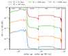 |
Fig. A.1. Ekman number calculated in the middle of the external convective envelope for different rotational periods during the lifetime of a 1.6 M⊙ star. |
Appendix B: Dynamical tidal dissipation
The energy luminosity of the dissipation of tidally excited progressive IGWs has been derived by Ahuir et al. (2021a). We refer the reader to this article for the details of the theoretical calculations that led to the following expression in the case of a star with a radiative core and a convective envelope:
 (B.1)
(B.1)
where rint is the radius of the radiative-convective interface. In a circular coplanar orbit, the energy luminosity can be expressed in terms of the complex part of the Love number as (Ogilvie 2014)
 (B.2)
(B.2)
 (B.3)
(B.3)
These equations can be used to derive the expression for the complex part of the Love number for the dissipation of tidally excited progressive IGWs:
 (B.4)
(B.4)
This expression can now be generalised to a three-layer structure (analogous to Sect. 4.3 of Ahuir et al. 2021a) to
 (B.5)
(B.5)
Appendix C: Comparison to Ahuir et al. (2021a)
To benchmark our implementation of the tidal dissipation prescriptions, as well as to estimate the robustness of the solutions for different stellar structure and evolution numerical codes, we compared our results to the results obtained by Ahuir et al. (2021a), who used stellar models with initial masses between 0.4 and 1.4 M⊙ using the stellar evolution code STAREVOL (Siess et al. 2000; Amard et al. 2016). In Ahuir et al. (2021a), the dissipation of the equilibrium tide is calculated assuming a thin convective envelope, assuming a constant density in the convective envelope, and approximating the mixing length by its maximum, such that the equilibrium tide dissipation becomes
 (C.1)
(C.1)
where Vc is the convective velocity, α and β are the ratio of the convective to the total radius and mass, respectively, and F(ωt) is the dependence of the turbulent viscosity on the tidal frequency (see Eq. 12). Assuming this formalism, the equilibrium tide is compared to the one calculated in Ahuir et al. (2021a) in Fig. C.1 (top panel). Here the dissipation is consistent between the MESA and STAREVOL models, except for the 1.4 M⊙ model where the dissipation is weaker in this study. This is due to the different opacity tables used in the two stellar evolution codes, resulting in lower densities in the small convective envelope.
For evolved stars with a large convective envelope, these approximations are no longer valid. Therefore, we computed the equilibrium tide dissipation taking realistic stellar profiles into account (see Sect. 2.3.1 and Barker 2020). The two different formalisms are shown in Fig. C.2. Here it can be seen that the equilibrium tide dissipation calculated in this study is significantly weaker than the one calculated in Ahuir et al. (2021a). As more approximations were made to estimate the equilibrium tide dissipation in Ahuir et al. (2021a), the dissipation of the equilibrium tide calculated in this study is more reliable.
In Fig. C.1 the tidal dissipation from IGWs is shown at the top for 1, 1.2, and 1.4 M⊙ stars and a 1 MJup companion on an orbit of 1 d, using both the STAREVOL models used in Ahuir et al. (2021a) and the MESA models used in this study. When performing this benchmark, a unit mistake was found in the numerical computations of Ahuir et al. (2021a), resulting in a reduction of the dynamical tide dissipation by roughly an order of magnitude compared to what was reported by Ahuir et al. (2021a). This has no significant impact on their conclusions. For the 1 and 1.2 M⊙ models the results are almost identical when using MESA and STAREVOL models. For the 1.4 M⊙ model, the dynamical tide dissipation are weaker in this study. This is because the star has a negligible convective envelope during the MS, and as the stellar evolution codes use different opacity tables, these regions are slightly different when using MESA or STAREVOL, resulting in different densities in these layers. During the further evolution of the stars, when the convective envelope grows again, the difference vanishes. Therefore, the ratio of the dynamical to equilibrium tidal dissipation remains roughly the same when using MESA or STAREVOL models. The results are in good agreement with those of Terquem et al. (1998), Goodman & Dickson (1998), and Barker & Ogilvie (2010). This validates our implementation in MESA and show that the results are robust for different stellar structure and evolution codes.
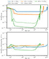 |
Fig. C.1. Complex part of the Love number for dynamical (Im(k22)IGW; upper plot) and equilibrium (Im(k22)eq following Eq. C.1; lower plot) tides, as a function of stellar age, for both the Ahuir et al. (2021a) results (dashed lines) and results from this study (solid lines). |
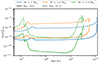 |
Fig. C.2. Complex part of the Love number for the equilibrium tide (Im(k22)eq), as a function of stellar age, for both the Ahuir et al. (2021a) formalism (Eq. C.1) and Eq. 10 (this study). |
Appendix D: Tidal dissipation evaluation for complementary masses of the stellar evolution grid
This section contains the tidal dissipation figures for the remaining stellar evolutionary models not illustrated in the main text. Their main patterns have been identified and explained in Sect. 4.5.
Appendix E: MESA inlist
The MESA (release-r23.05.1) inlist we used in this study is reported hereafter. Here ‘initial_mass = mass’ refers to the initial mass of the star and ‘Blocker_scaling_factor = Blocker’ to the Blöcker scaling factor for AGB mass-loss; ηblöcker = 0.05 for masses below 2 M⊙ and ηblöcker = 0.1 for masses above 2 M⊙.
&star_job

  create_pre_main_sequence_model = .true.

  ! network
  auto_extend_net = .true.
  h_he_net = 'basic.net'
  co_net = 'co_burn.net'
  adv_net = 'approx21.net'

  ! opacities
  initial_zfracs = 6 ! for L03 solar scaling

/ !end of star_job namelist

&kap

  Zbase = 0.0134d0

  use_Type2_opacities = .true.
  kap_file_prefix = 'a09'
  kap_CO_prefix = 'a09_co'
  kap_lowT_prefix = 'AESOPUS'
  AESOPUS_filename = 'AESOPUS_AGSS09.h5'
/ ! end of kap namelist

&controls

  log_L_lower_limit = -1

  varcontrol_target = 1d-4
  min_timestep_limit = 1d-10

  initial_mass = Mass
  initial_z = 0.0134d0

  mixing_length_alpha = 1.931
  MLT_option = 'Henyey'

  atm_option = 'T_tau'
  atm_T_tau_relation = 'Eddington'
  atm_T_tau_opacity = 'fixed'

  cool_wind_RGB_scheme = 'Reimers'
  cool_wind_AGB_scheme = 'Blocker'
  RGB_to_AGB_wind_switch = 1d-4
  Reimers_scaling_factor = 0.477d0
  Blocker_scaling_factor = Blocker

  set_min_D_mix = .true.
  min_D_mix = 1d1

  num_cells_for_smooth_brunt_B = 10
  threshold_for_smooth_brunt_B = 0.1

  num_cells_for_smooth_gradL
    _composition_term = 10
  threshold_for_smooth_gradL
    _composition_term = 0.02

  report_solver_progress = .true.
  use_gold_tolerances = .false.

  solver_iters_timestep_limit = 20
  solver_max_tries_before_reject = 30

  energy_eqn_option = 'dedt'
  convergence_ignore_equL_residuals = .true.
  corr_coeff_limit = 1d-1
  max_abs_rel_run_E_err = 1d-1
  warn_when_large_rel_run_E_err = 1d-3
  ignore_too_large_correction = .true.
  scale_max_correction = 1d-2
  ignore_min_corr_coeff_for
    _scale_max_correction = .true.
  ignore_species_in_max_correction = .true.
  use_superad_reduction = .true.

  log_directory = 'LOGS'
  photo_interval = 10
  max_num_profile_models = 100000
  profile_interval = 10
  history_interval = 1
  terminal_interval = 1
  write_header_frequency = 1

/ ! end of controls namelist
All Figures
|
Fig. 1. Brunt-Väisälä (N; in blue), Lamb (for l = 2; S2; in orange), and tidal (ωt; in green) frequencies for a planetary companion orbiting an RGB star with MZAMS = 1 M⊙ at a distance of 1 AU. The colours mark the regions where the different types of waves can be excited (see the main text for details). |
| In the text | |
|
Fig. 2. Schematic representation of the radiative and convective shells in the case of the three-layer structure used in this study. Radii are not to scale for a real stellar structure (see the Kippenhahn diagrams, e.g. Fig. 5). |
| In the text | |
|
Fig. 3. Hertzsprung-Russell diagram of the stellar evolutionary models studied here. The models start in the PMS and are evolved up to the WD phase. Different colours indicate a different ZAMS mass, as indicated in the box in the left-bottom corner. |
| In the text | |
|
Fig. 4. Critical period, Pc = 1/νc, for different stellar masses. The different colours represents the same model as in Fig. 3. The filled regions indicate where the g-waves are excited as progressive IGWs. |
| In the text | |
|
Fig. 5. Kippenhahn diagram for a MZAMS = 1 M⊙ star. The brown hatched region represents convective layers, and the yellow dotted region represents radiative layers. The upper layer represents the radius of the star. Stellar evolutionary phases (PMS to WD) are indicated. |
| In the text | |
|
Fig. 6. Complex part of the Love number (Im(k22)) for both equilibrium (blue) and dynamical (red) tides (left axis) and stellar radius (brown; right axis) as a function of stellar age for a MZAMS = 1 M⊙ star with a 1 MEarth companion at 1 AU. Stellar evolutionary phases (PMS to WD) are indicated. |
| In the text | |
|
Fig. 7. Different components appearing in the dissipation of the dynamical tide (Eq. (13)) as a function of stellar age. The change in radius of the radiative-convective boundary is represented in blue, the change in stellar mass in orange, the change in local density at the boundary in green, the change in tidal forcing compared to changes in the stellar radius in red, and change in the derivative of the Brunt-Väisälä frequency in purple. Stellar evolutionary phases (PMS to WD) are indicated. |
| In the text | |
|
Fig. 8. Complex part of the Love number for the equilibrium tide (Im(k22)eq) as a function of the orbital period and stellar age for a MZAMS = 1 M⊙ star. R⋆ (in brown) represents the orbital period on which a planet orbits at the surface of the star, and the Roche limit is given in purple. Changes in the stellar evolutionary phase are indicated with ticks on the upper axis. |
| In the text | |
|
Fig. 9. Complex part of the Love number for the dynamical tide (Im(k22)IGW) as a function of orbital period and stellar age for a MZAMS = 1 M⊙ star. The critical period, Pc, above which companions excite progressive IGWs, is shown in orange. R⋆ (in brown) represents the orbital period on which a planet orbits at the surface of the star, and the Roche limit is given in purple. Changes in the stellar evolutionary phase are indicated with ticks on the upper axis. |
| In the text | |
|
Fig. 10. Ratio of the complex parts of the Love number for the dynamical to equilibrium tide (Im(k22)IGW/Im(k22)eq) as a function of the orbital period and stellar age for a MZAMS = 1 M⊙ star. The critical period, Pc, above which companions excite progressive IGWs, is shown in orange. R⋆ (in brown) represents the orbital period on which a planet orbits at the surface of the star, and the Roche limit is given in purple. Changes in the stellar evolutionary phase are indicated with ticks on the upper axis. |
| In the text | |
|
Fig. 11. Internal structure and tidal dissipation evolution for a MZAMS = 2 M⊙ star. Top left: Kippenhahn diagram. The brown hatched regions represent convective layers, and the yellow dotted region represents radiative layers. Stellar evolutionary phases (PMS to WD) are indicated. Top right, bottom left, and bottom right: Complex part of the Love number for the equilibrium tide (Im(k22)eq), the dynamical tide (Im(k22)IGW), and the ratio of the dissipations of the dynamical tide to the dissipation of the equilibrium tide (Im(k22)IGW/Im(k22)eq), respectively, as a function of stellar age and orbital period. The Roche limit is shown in purple, the critical period (1/νc; see Eq. 6) in orange, and the period at which a planet orbits at the stellar radius in brown. Changes in the stellar evolutionary phase are indicated with ticks on the upper axis. |
| In the text | |
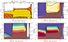 |
Fig. 12. Same as Fig. 11, but for a MZAMS = 3.5 M⊙ star. |
| In the text | |
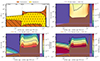 |
Fig. 13. Same as Fig. 11, but for a MZAMS = 4 M⊙ star. |
| In the text | |
|
Fig. A.1. Ekman number calculated in the middle of the external convective envelope for different rotational periods during the lifetime of a 1.6 M⊙ star. |
| In the text | |
|
Fig. C.1. Complex part of the Love number for dynamical (Im(k22)IGW; upper plot) and equilibrium (Im(k22)eq following Eq. C.1; lower plot) tides, as a function of stellar age, for both the Ahuir et al. (2021a) results (dashed lines) and results from this study (solid lines). |
| In the text | |
|
Fig. C.2. Complex part of the Love number for the equilibrium tide (Im(k22)eq), as a function of stellar age, for both the Ahuir et al. (2021a) formalism (Eq. C.1) and Eq. 10 (this study). |
| In the text | |
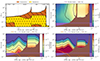 |
Fig. D.1. Same as Fig. 11, but for a MZAMS = 1.2 M⊙ star. |
| In the text | |
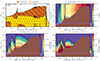 |
Fig. D.2. Same as Fig. 11, but for a MZAMS = 1.4 M⊙ star. |
| In the text | |
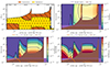 |
Fig. D.3. Same as Fig. 11, but for a MZAMS = 1.6 M⊙ star. |
| In the text | |
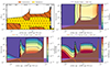 |
Fig. D.4. Same as Fig. 11, but for a MZAMS = 1.8 M⊙ star. |
| In the text | |
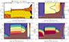 |
Fig. D.5. Same as Fig. 11, but for a MZAMS = 2.5 M⊙ star. |
| In the text | |
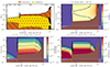 |
Fig. D.6. Same as Fig. 11, but for a MZAMS = 3 M⊙ star. |
| In the text | |
Current usage metrics show cumulative count of Article Views (full-text article views including HTML views, PDF and ePub downloads, according to the available data) and Abstracts Views on Vision4Press platform.
Data correspond to usage on the plateform after 2015. The current usage metrics is available 48-96 hours after online publication and is updated daily on week days.
Initial download of the metrics may take a while.