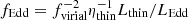
| Issue |
A&A
Volume 689, September 2024
|
|
|---|---|---|
| Article Number | A128 | |
| Number of page(s) | 8 | |
| Section | Extragalactic astronomy | |
| DOI | https://doi.org/10.1051/0004-6361/202451249 | |
| Published online | 06 September 2024 | |
Size matters: are we witnessing super-Eddington accretion in high-redshift black holes from JWST?
1
Dipartimento di Scienza e Alta Tecnologia, Università degli Studi dell’Insubria, via Valleggio 11, 22100 Como, Italy
2
INFN, Sezione di Milano-Bicocca, Piazza della Scienza 3, 20126 Milano, Italy
3
INAF, Osservatorio Astronomico di Roma, Via Frascati 33, 00040 Monte Porzio Catone, Italy
4
Institut d’Astrophysique de Paris, UMR 7095, CNRS and Sorbonne Université, 98 bis boulevard Arago, 75014 Paris, France
5
Dipartimento di Fisica “G. Occhialini”, Università degli Studi di Milano-Bicocca, Piazza della Scienza 3, 20126 Milano, Italy
6
Instituto de Estudios Astrofísicos, Facultad de Ingeniería y Ciencias, Universidad Diego Portales, Avenida Ejercito Libertador 441, Santiago, Chile
Received:
25
June
2024
Accepted:
15
July
2024
Abstract
Observations by the James Webb Space Telescope of the Universe at z ≳ 4 have shown that massive black holes (MBHs) appear to be extremely overmassive compared to the local correlation for active galactic nuclei. In some cases, these objects might even reach half the stellar mass inferred for the galaxy. It has become a great challenging for theoretical models to understand how these objects formed and grew to these masses. Different ideas range from heavy seed to super-Eddington accretion phases. We take a different approach and try to infer how accurate these MBH mass estimates are and whether we really need to revise our physical models. By considering how the emerging spectrum (both the continuum and the broad lines) of an accreting MBH changes close to and above the Eddington limit, we infer a much larger uncertainty in the MBH mass estimates relative to that of local counterparts. The uncertainty is up to an order of magnitude. We also infer a potential preference for lower masses and higher accretion rates, which i) moves accreting MBHs closer to the local correlations, and ii) might indicate that we witness a widespread phase of very rapid accretion for the first time.
Key words: accretion, accretion disks / black hole physics / galaxies: active / galaxies: high-redshift
Corresponding author; This email address is being protected from spambots. You need JavaScript enabled to view it. .
© The Authors 2024
 Open Access article, published by EDP Sciences, under the terms of the Creative Commons Attribution License (https://creativecommons.org/licenses/by/4.0), which permits unrestricted use, distribution, and reproduction in any medium, provided the original work is properly cited.
This article is published in open access under the Subscribe to Open model. This email address is being protected from spambots. You need JavaScript enabled to view it. to support open access publication.
1. Introduction
Massive black holes (MBHs) are ubiquitously found to inhabit the centre of massive galaxies up to redshift z ≳ 6 (e.g. Fan et al. 2006, 2023; Mortlock et al. 2011; Bañados et al. 2018; Maiolino et al. 2023), with masses in the range ∼105 − 1010 M⊙. Observationally, they are commonly identified via gas accretion through the conversion of gravitational energy into radiation, which makes them shine as active galactic nuclei (AGN). They sometimes also produce powerful collimated jets.
MBHs are expected to gain most of their mass via radiatively efficient accretion (Soltan 1982; Marconi et al. 2004), which means that they likely formed from lower-mass black hole seeds (see e.g. Inayoshi et al. 2020 and Volonteri et al. 2021 for a review).
With the advent of the James Webb Space Telescope (JWST), we have pushed the observational limit to deep in the dark ages, detecting galaxies up to z ∼ 14 (Carniani et al. 2024). Some of these galaxies also hosted MBHs, which appear to challenge most MBH formation mechanisms, unless an initially heavy seed is assumed (104 − 105 M⊙; see e.g. Begelman et al. 2008; Begelman 2010; Volonteri & Begelman 2010; Choi et al. 2013; Coughlin & Begelman 2024) as well as continuous growth at the Eddington limit. Theoretical models are further challenged by the large abundance of these (candidate) objects (e.g. Harikane et al. 2023; Maiolino et al. 2023; Greene et al. 2024). This abundance implies that the formation efficiency of massive seeds is far higher than what is found in theoretical models. Several studies have shown that this issue can be alleviated when the plausibility of accretion above the Eddington limit is considered (e.g., Lupi et al. 2016, 2024; Pezzulli et al. 2016; Regan et al. 2019; Massonneau et al. 2023; Shi et al. 2024), which can compensate for the stunted growth in low-mass galaxies (see, e.g. Anglés-Alcázar et al. 2017). In addition to the mass of these MBHs, another important difference with the local population is that these MBHs seem to be extremely massive compared to their galaxy hosts. Their masses lie well above the local correlations (Farina et al. 2022; Maiolino et al. 2023; Yue et al. 2024; Stone et al. 2024) and in some cases, they even exceed half the total stellar mass (Juodžbalis et al. 2024). We note, however, that an important role in the comparison is also played by the galaxy mass employed, either the stellar mass, as in the recent JWST results, or the dynamical mass, as in the case of ALMA1 observations (Decarli et al. 2018; Izumi et al. 2021; Farina et al. 2022). The most promising theoretical solutions to explain these systems consider i) a somewhat extremely efficient heavy seed formation at high redshift and an efficient suppression of star formation by the accreting MBH, ii) a strong observational bias (Li et al. 2024), or iii) a population of primordial MBHs (Ziparo et al. 2022; Dolgov 2024). Despite these efforts, a clear consensus is still lacking to date, in part because of the large uncertainties on the stellar mass and (potentially) on the MBH mass. The second possibility is rarely considered. The MBH mass at these redshifts is commonly inferred through the single-epoch method, employing the virial theorem combined with the correlations between the broad Hα, Hβ, or MgII line widths and luminosities, and the emission properties of the continuum emitted by the innermost regions of the accretion disc. These correlations have been calibrated in the local Universe (z ≲ 0.3 Vestergaard & Osmer 2009; Bentz et al. 2013; Reines et al. 2013; Reines & Volonteri 2015) and are then extrapolated to high redshift.
Recently, King (2024) pointed out that for close-to-Eddington or super-Eddington accreting MBHs (i) the emission from the accretion disc would be beamed by multiple scatterings within the funnel created by a central thickening of the disc itself, and (ii) the broad line regions (BLRs) would not be virialized, being mostly dominated by outflows. Under these conditions, King (2024) demonstrated that the inferred MBH mass estimates would be artificially biased towards high values, and they argued that this effect might be particularly relevant for high-redshift AGN. Another potential source of bias could instead result from an inaccurate estimate of the BLR size, as suggested by recent reverberation mapping campaigns (including the SEAMBH (Du et al. 2014) and the SDSS-RM (Grier et al. 2017)) of multiple highly accreting MBHs (Martínez-Aldama et al. 2019), and also by the GRAVITY collaboration (Abuter et al. 2024).
In particular, these campaigns demonstrated that the time lag of the Hβ line, which is directly associated with the size of the BLR, depends on the accretion rate of the MBH, and it is shorter for accretion rates above fEdd ∼ 0.3 (Wang et al. 2014, W14 hereafter). The proposed interpretation of this effect is radiation pressure, which for accretion rates close and above the Eddington limit thickens the accretion disc. A thicker disc like this is better described by the slim-disc solution (Abramowicz et al. 1988) than by a more standard radiatively efficient Shakura & Sunyaev (1973, SS hereafter) disc, and this results in a lower flux of ionising photons that reach the BLR clouds compared to a radiatively efficient AGN with an identical optical spectrum. In these conditions, the BLR splits into unshadowed and shadowed regions, the latter receiving fewer photons and shrinking in size. This results in a net shorter lag.
Motivated by these results, in this work we explore the effect of a varying BLR size, based on the results described above and on a fully physical approach, on the inferred MBH masses in the most challenging high-redshift sources observed by JWST to date. In particular, we account for the possibility that the observed luminosities might be the result of a lower-mass highly accreting MBH, with the aim of assessing potential biases in the MBH mass estimates.
The paper is organised as follows. In Sect. 2 we describe our procedure for estimating the MBH mass. In Sect. 3 we present our results, and in Sect. 4 we discuss potential caveats in the analysis and draw our conclusions.
2. Methods
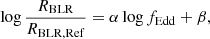
In order to test how relevant the evolution of the BLR size with the Eddington ratio is in high-redshift systems, we built a theoretical model of the accretion disc and the BLR emissions based on the electromagnetic spectrum of a slim disc, as defined by the AGNSLIM model in XSPEC (Kubota & Done 2019). Of the many parameters available in the model, we only considered the impact of the three main ones: the MBH mass MBH, the Eddington ratio Lthin/LEdd ≡ ηthin ṀBHc2/LEdd, with Lthin and ηthin being the bolometric luminosity and the radiative efficiency of an SS disc, and the MBH spin aBH, leaving the others at their default value. We sampled 6250 different combinations, with 25 logarithmically spaced MBH masses between 105 and 1010 M⊙, 25 logarithmically spaced Eddington ratios in the range 0.01 − 103, and 10 linearly spaced values of the MBH spin between 0 and 0.998. The spectrum covered the energy range 0.1 eV – 100 keV, corresponding to a wavelength range 0.12 Å–12.4 μm, in 1000 logarithmically spaced bins.
After the spectra were generated, we listed for each combination the luminosity at 5100 Å (λLλ) and the ionising luminosity Lion above E > 0.1 keV (soft-X; Kwan & Krolik 1979). The latter is needed to determine the broad-line emission from the disc properties (see, e.g. Osterbrock & Ferland 2006). For consistency with Kubota & Done (2019), we normalised the spectral bolometric luminosity to the value estimated from the numerical integration of the slim-disc solution by Sadowski (2011). This normalisation yielded the effective radiative efficiency η for each combination of the three model parameters, which we use in the remainder of the paper to determine L/LEdd = η/ηthinLthin/LEdd. With this table, we then built a theoretical model for the BLR emission to be compared with observations. In particular, the observed quantities we considered are the broad-line width (either Hα or Hβ) and the luminosity (either the Hα luminosity or the luminosity at 5100 Å), according to the values reported in the corresponding observational works (Harikane et al. 2023; Maiolino et al. 2023; Übler et al. 2023; Greene et al. 2024), both with their associated uncertainties σ.
Our model is defined as listed below.
-
Given a specific combination of MBH, Lthin/LEdd and aBH, we extracted L5100 Å and Lion via tri-linear interpolation on our table.
-
For simplicity, we made no specific assumption about the cloud properties in the BLR, and generically assumed that they are homogeneously distributed around the central MBH (Wang et al. 2014)2. Following W14, we assumed that self-shadowing is negligible within the funnel, which is defined by an aperture
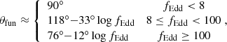 (1)
(1)where
 , and that the ionising radiation emitted within this solid angle directly impinges on the BLR clouds. Assuming an intrinsic spectrum with angular distribution dF/dθ ∝ cos θ, we then determined the broad-line emission from clouds within the funnel solid angle assuming the local correlation (Greene & Ho 2005),
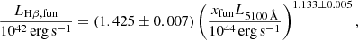 (2)
(2)where xfun is the fraction of the total ionising flux within the funnel. Outside the funnel, instead, we modelled self-shadowing through Eq. (19) in W14
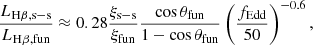 (3)
(3)where ξs − s and ξfun are the anisotropic factors for Hβ emission from the BLR clouds in the self-shadowed region and within the funnel, respectively, because these values are completely unconstrained, but for pole-on observers (where they are both equal to unity). We assumed for simplicity that they are always of the same order and removed them from the equation. The total Hβ luminosity was finally estimated as LHβ = LHβ, fun + LHβ, s − s. In order to determine the Hα luminosity, we assumed the standard scaling from Greene & Ho (2005)
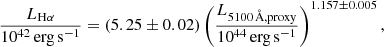 (4)
(4)where
 (5)
(5)We note that when the broad-line flux or luminosity are not reported, as in the case of Yue et al. (2024), we directly compared L5100 Å from our model with the observed data.
-
The last piece of information we need for the model is the full width at half maximum (FWHM) of the broad lines, which we determined by assuming virial equilibrium in the BLR, which gives
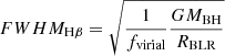 (6)
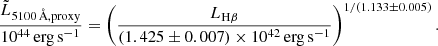
(6)for the Hβ line, where fvirial takes the unknown inclination, geometry, and kinematics of the BLR into account. We considered as our fiducial case fvirial = 1.075 (Reines & Volonteri 2015), but also explored a case in which fvirial ∝ (FWHMline, obs)−k (Mejía-Restrepo et al. 2018, MR18 hereafter), with k = 1 (Hα) or k = 1.17 (Hβ). In order to estimate RBLR, we employed the relations derived by Martínez-Aldama et al. (2019),
 (7)
(7)which takes the self-shadowing of the BLR into account. For the fiducial model, we set α = −0.143, β = −0.136, and assumed RBLR, Ref as the reference Hβ BLR size estimate by Bentz et al. (2013),
 (8)
(8)In the MR18 case, we instead employed α = −0.283, β = −0.228, and
 . For sources whose MBH mass was estimated from Hα, we finally converted FWHMHβ into the FWHMHα through the Bentz et al. (2013) relation,
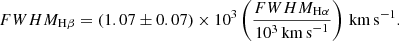 (9)
(9)
In order to compare our model predictions with observations, we employed a Markov chain Monte Carlo (MCMC) algorithm as implemented in the EMCEE package (Foreman-Mackey et al. 2013). We considered as our observational sample the sources identified by Harikane et al. (2023), Maiolino et al. (2023), Yue et al. (2024), Übler et al. (2023), and Greene et al. (2024) in the redshift range 4 ≲ z ≲ 7. The likelihood ℒ for the MCMC was defined through
![Mathematical equation: $$ \begin{aligned} \ln \mathcal{L} = -\frac{1}{2} \sum _i \left[ \frac{(Y_i-\bar{Y}_i)^2}{s_i^2} + \ln (2\pi s_i^2)\right], \end{aligned} $$](/articles/aa/full_html/2024/09/aa51249-24/aa51249-24-eq12.gif) (10)
(10)
where Yi is the observed broad-line FWHM, the luminosity,  is the value predicted by our model, and si is the uncertainty in the observed data (assumed Gaussian). The parameters of our model that we aimed to constrain are MBH, Lthin/LEdd, and aBH. As priors, we assumed a log-flat distribution for MBH and Lthin/LEdd over the intervals [5, 10] and [− 3, 3], respectively, and a uniform distribution for aBH between 0 and 0.998. We ran the MCMC for 10 000 steps employing 32 walkers3. In order to incorporate the uncertainties in the correlations used by our model, every time we employed one of the relations above, we sampled the slope and normalisation from a Gaussian distribution centred on the best-fit value and with σ defined by the uncertainty of the fit4. This choice ensured a proper coverage of the parameter space, even with a very limited dataset given by only two values. In the case of an FWHM-dependent virial factor, we randomly sampled the virial factor for each source before starting the MCMC from a Gaussian distribution centred on the observed broad-line FWHM with the observed uncertainty, and kept it constant throughout the optimisation procedure, which is in line with the correlation found by Mejía-Restrepo et al. (2018).
3. Results
3.1. Model validation
Before running the MCMC with the fiducial model described in the previous section, we decided to validate our procedure by neglecting the effects due to the accretion disc transition to a slim disc. In practice, (i) we employed
 (11)
(11)
in Eq. (6), as was done in Reines & Volonteri (2015), (ii) we inferred the broad-line luminosities from the scaling relations in Bentz et al. (2013, see also Eqs. (2) and (4)), using our tabulated value for L5100 Å, and (iii) we assumed a constant fvirial = 1.075 as in Reines & Volonteri (2015). With these assumptions, we found our best parameters to be in line with those in the published works, as shown in Fig. 1. The inset shows the remarkable agreement of our procedure with the data by Reines & Volonteri (2015). The only mild discrepancy is in the data by Greene et al. (2024), where the estimates show a somewhat larger scatter around the 1:1 relation. The systematic small shift of the Harikane et al. (2023, above) and Maiolino et al. (2023, below) is likely related to the information provided in the respective papers. Maiolino et al. (2023) reported the Hα flux, which was then converted into luminosity assuming the cosmology and redshift reported in the discovery paper, while Harikane et al. (2023) directly reported the broad line luminosity. We refer to the MBH masses obtained with this procedure as ‘validation’ in the following.
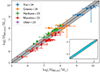 |
Fig. 1. MBH estimates from the MCMC for the validation run against the MBH mass reported in the observational studies. The black line corresponds to the 1:1 relation, and the grey shaded area is 0.3 dex wide. The dots correspond to the MBHs in Yue et al. (2024, blue), Greene & Ho (2005, orange), Harikane et al. (2023, green), Maiolino et al. (2023, red), and Übler et al. (2023, purple). In the inset, we show the results obtained for the Reines & Volonteri (2015) data as cyan crosses. |
In general, we find that the spin is very poorly constrained by our MCMC because of the limited number of observational data we have and the moderate dependence on its value, whereas the MBH mass and L/LEdd are typically well determined. As an example of the robustness of our procedure, we report in Fig. 2 the corner plot obtained for J1030+0524 from Yue et al. (2024), which is one of the most massive sources in the sample and is also one of the few validation cases in which the posterior distribution of the MBH spin exhibits a peak rather than being almost flat. The blue lines in the corner plot correspond to the estimates from the literature, which agree well with our estimate.
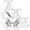 |
Fig. 2. Corner plot resulting from the MCMC validation run on J1030+0524 (Yue et al. 2024) for the three physical parameters of the model MBH, L/LEdd (obtained by rescaling Lthin/LEdd as described in Sect. 2), and aBH. The blue lines correspond to the values reported in the original work. |
In the left panel of Fig. 3, we show the same plot as in Fig. 1, but for the slim-disc model. We clearly observe that the fiducial case is close to the 1:1 relation, but it is typically offset of about 0.5 dex towards lower values compared to those reported in the literature, with correspondingly higher accretion rates that are often super-Eddington. Because of the additional dependence of the virial factor on the broad-line FWHM, the MR18 case results in even lower MBH masses. The Ṁ/ṀEdd ratio is shown in the right panel, where ṀEdd ≡ 10LEdd/c2, assuming the fiducial and the MR18 cases of our slim-disc model (red dots and purple squares, respectively) and the validation run (black crosses). Despite the differences in the two slim-disc models, we find that the distribution of Eddington ratios is quite similar, with a preference for higher accretion rates in the least massive MBHs. Consistently with the lower MBH masses reported in the left panel, MR18 almost always shows super-Eddington rates, with values between 10 and a 100 times Eddington. Interestingly, the most massive MBHs from Yue et al. (2024) also show super-Eddington accretion rates that are well above the Eddington limit, which might indicate an ineffective self-regulation of their growth via feedback processes. Another interesting aspect is that even in the validation run, some MBHs seem to lie above the Eddington limit, especially those with the lowest masses, suggesting that the estimate of their properties according to the local correlations might be biased towards higher MBH masses. Finally, we note that it is hard to distinguish high accretion rates from more typical cases because the luminosity of these objects would never exceed a few times the Eddington luminosity (5–10) even in the most extreme cases.
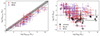 |
Fig. 3. In the left panel, we show the MBH mass estimates (as in Fig. 1), but for our full model, with the estimates of the entire sample shown as red dots (fiducial) and purple squares (MR18). The dashed black line is plotted to guide the eye and corresponds to a 0.5 dex offset relative to the 1:1 relation. In the right panel we show instead the Eddington ratio distribution for our fiducial model (red dots), the MR18 case (purple squares), and the validation run (black crosses) as a function of the estimated MBH mass. The thick dashed grey line corresponds to the Eddington limit. |
As we discussed above, the MBH and the Eddington ratio in our analysis are typically constrained within one order of magnitude, even with the slim-disc model, whereas the MBH spin is almost always uniformly distributed. This suggests that our model can accommodate the observed data almost independently of the spin. At super-Eddington rates this is expected, as the effective radiative efficiency does not depend on the spin (Madau et al. 2014). Below the Eddington limit, this instead suggests that the available information is not sufficient to clearly distinguish the spin from the other two parameters.
Finally, we can assess how the correlations between MBHs and their hosts would change based on the results of our full model. The results are shown in Fig. 4 for the fiducial (left panel) and MR18 (right panel) cases. Our estimates are closer to the local relations, and this effect is more relevant for MR18. Interestingly, this decrease does not completely realign the MBHs with the local correlations, but suggests that the current estimates, especially for the lowest-mass MBHs observed, could have a much larger uncertainties than reported in the literature, and that their offset relative to the local MBH mass-stellar mass correlation should be considered in the light of what we found in this work, in addition to observational biases.
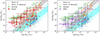 |
Fig. 4. MBH mass–stellar mass relation for the sources in our sample. We show the local AGN from Reines & Volonteri (2015) as blue stars and orange diamonds, with the underlying shaded area correspond to the 1σ and 2σ uncertainties around the best fits to the local samples (grey and cyan for inactive and active galaxies, respectively). The original data from the literature are shown as green circles, whereas our new estimates are reported as red dots (left panel) and purple crosses (right panel) for the two virial factors considered. For completeness, we also show as the dotted magenta lines constant mass ratios of 0.01 and 0.1. |
Even though not reported here (as no estimate of the stellar mass is available), we performed our analysis also on the sources by Matthee et al. (2024), finding similar variations in the MBH mass to those just discussed. In order to determine whether the inclusion of a slim-disc emission produced a rigid shift in the MBH masses for the local sources as well, we reanalysed the Reines & Volonteri (2015) sample using our fiducial model. We found that a decrease in the inferred MBH mass was also present in the local AGN sample on average, but with variations not larger than 0.2 dex, which is about a factor of 3 smaller than the intrinsic uncertainty by Reines & Volonteri (2015), and typically much smaller than the 0.5 dex found in the high-redshift sample.
3.2. Spectra of active galactic nuclei
As a final check of our procedure, we built synthetic MBH emission spectra for the analysed sources and employed all of the three models considered in this work. The best parameters to build the spectra are defined as the average of the ten evaluations of our MCMC with the maximum likelihood. For each model, we extracted the continuum spectrum from our tables and added the emission of the broad line (except for the sources in Yue et al. 2024, where we employed the luminosity at 5100 Å). In order to consistently compare this with observed spectra, we also accounted for dust extinction following the attenuation law by Calzetti et al. (2000), assuming RV = 4.05 for the source by Harikane et al. (2023), and the Small Magellanic Cloud value RV = 2.74 for the sources by Maiolino et al. (2023) and Greene et al. (2024), to be consistent with the assumptions in the different studies. For the sources observed in the EIGER program (Yue et al. 2024), we did not include any attenuation. The results are reported in Fig. 5 for four selected sources: CEERS_02782 (Harikane et al. 2023), JADES_000954 (Maiolino et al. 2023), J0100+2802 (Yue et al. 2024), and UNCOVER_13821 (Greene et al. 2024). Our models always clearly recover the spectral properties of the sources, both the continuum region and the broad Hα line intensity and width, independently of the assumptions. The only peculiar case is J0100+2802, where the complexity of the broad Hβ line profile, not symmetric and with potential indications of offset components, together with the missing modelling of the iron emission in our model, does not allow us to recover the exact spectrum. Nonetheless, we find that our model reproduces the power-law continuum very well, but for a mildly higher normalisation, which is simply due to the use in our MCMC of the total continuum luminosity reported in Yue et al. (2024) instead of the contribution of the power-law component alone5. This confirms i) the robustness of our procedure, and ii) that the dependence of the BLR emission on the accretion disc structure and the Eddington ratio is somewhat degenerate, resulting in potentially significant differences in the MBH mass estimate when it is not properly taken into account.
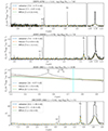 |
Fig. 5. Reconstructed spectra for four selected sources in our sample: CEERS_02782, JADES_000954, J0100+2802, and UNCOVER_13821. The observed spectra (obtained from the public data release of the different programs, except for the UNCOVER source, which was extracted from the published paper) are shown as solid black lines (the right panel shows a zoom on the Hα line), the dashed blue, dash-dotted orange, and dotted green lines refer to our validation, to the fiducial, and to the MR18 models, respectively. The vertical cyan line in J0100+2802 corresponds to λ = 5100 Å redshifted to the observer frame, which we used to constrain the models. The grey line corresponds to the power-law continuum component from the fit by Yue et al. (2024). All but the UNCOVER source report absolute fluxes, whereas in the UNCOVER case, the flux is normalised to the luminosity at 2500 Å, as was done in Greene et al. (2024). The numbers reported in the legend correspond to the parameters employed for each model log(MMBH/M⊙), log(L/LEdd), and aBH, whereas the mass estimates above each panel correspond to those in the corresponding discovery papers. |
4. Discussion and conclusions
We have built a semi-empirical model of the BLR emission of MBHs in different accretion regimes. By combining theoretical models of the emission of thin and slim accretion discs (Kubota & Done 2019) with observed scaling relations at low redshift, which naturally account for different accretion regimes, we built a versatile model that can be applied to high-redshift sources such as those recently observed by JWST.
We have incorporated our model in a MCMC tool that we used to re-analyse some recent candidate MBHs from JWST observations. Our results showed that in many cases, a super-Eddington accreting MBH is preferred with respect to the standard SS accretion disc, which translates into MBH masses that are lower by up to an order of magnitude. This is in contrast with local sources such as those by Reines & Volonteri (2015), where more than 95 percent of the AGN are sub-Eddington and our fiducial model almost perfectly recovers the masses reported in the literature. We also note that the missing detection in X-rays of many of these sources might be compatible with a slim accretion disc, but we leave this aspect to future investigations.
Despite the extreme relevance of potentially detecting and identifying highly super-Eddington sources, it is unclear whether this accretion phase can be sustained over long timescales (see, e.g. Regan et al. 2019; Massonneau et al. 2023; Lupi et al. 2024). In particular, there is a potential degeneracy between the MBH mass and the Eddington ratio, and we cannot completely exclude a biased preference for super-Eddington accretion in low-mass systems. Because of the radiation trapping in the innermost regions of the accretion disc, which suppresses the increase in ionising and bolometric luminosity, a slim-disc model has more freedom to match the combination of FWHM and luminosities of some of these sources compared to a standard SS disc, without being for this reason more physically plausible. Moreover, any difference in the structure of the BLR (different geometry of the clouds, different density, etc.), as well as different inclinations, might in principle produce similar effects without requiring a highly super-Eddington accretion rate. All these uncertainties enter the virial factor, whose definition can produce variations in the MBH mass estimate of up to one order of magnitude, as we have shown here, especially in high-redshift systems for which only a limited amount of information is available.
As for our model, King (2024) pointed out that high-redshift MBH mass estimates could be biased toward too high values. Differently from King (2024), in our analysis we did not consider any radiation beaming, nor the possibility that the BLR might be mainly dominated by non-virialized outflows. Considering the more likely super-Eddington nature of many observed sources and the fact that in these conditions, radiation beaming as well as nuclear outflows become more significant, we expect the uncertainties in the mass estimate to become even larger. Unfortunately, the limited data available do not allow us to confirm whether a bias in the mass is real and if this bias might realign MBHs with the local correlation. However, it provides some insights into the impact of detailed accretion disc physics on the MBH mass estimates. In the future, we will incorporate additional information from the observed spectra, which will help us to better constrain the actual mass through our physically motivated model.
Atacama Large Millimiter Array.
This is a very simplistic assumption, as both the cloud angular distribution and their maximum distance from the source are completely unconstrained. Previous studies hinted at a common disc-like geometry for the BLR (e.g. Wills & Browne 1986; Collin-Souffrin 1987; Runnoe et al. 2013). We stress that a flatter BLR would enhance the self-shadowing effect.
This number of steps corresponds to about 100 auto-correlation timescales, which is sufficient to guarantee a robust optimisation.
When the uncertainties were asymmetric, we approximated the distribution as a Gaussian distribution, with σeff the average between the two uncertainties.
As a check, we re-ran our MCMC on J0100+2802 with a 5% lower luminosity at 5100 Å (consistent with the expected power-law contribution), and found that with almost identical MBH mass estimates, the agreement with the power-law fit was remarkable, as expected.
Acknowledgments
AL and AT acknowledge support from PRIN MUR “2022935STW”. CM acknowledges support from Fondecyt Iniciacion grant 11240336 and the ANID BASAL project FB210003. AL thanks the organisers of the “Massive black holes in the first billion years” conference Micheal Tremmel and John Regan, as well as Ricarda Beckmann, Amy Reines, and Alberto Sesana for useful discussions that inspired this work.
References
- Abramowicz, M. A., Czerny, B., Lasota, J. P., & Szuszkiewicz, E. 1988, ApJ, 332, 646 [Google Scholar]
- Abuter, R., Allouche, F., Amorim, A., et al. 2024, Nature, 627, 281 [NASA ADS] [CrossRef] [Google Scholar]
- Anglés-Alcázar, D., Faucher-Giguère, C.-A., Quataert, E., et al. 2017, MNRAS, 472, L109 [Google Scholar]
- Bañados, E., Venemans, B. P., Mazzucchelli, C., et al. 2018, Nature, 553, 473 [Google Scholar]
- Begelman, M. C. 2010, MNRAS, 402, 673 [NASA ADS] [CrossRef] [Google Scholar]
- Begelman, M. C., Rossi, E. M., & Armitage, P. J. 2008, MNRAS, 387, 1649 [NASA ADS] [CrossRef] [Google Scholar]
- Bentz, M. C., Denney, K. D., Grier, C. J., et al. 2013, ApJ, 767, 149 [Google Scholar]
- Calzetti, D., Armus, L., Bohlin, R. C., et al. 2000, ApJ, 533, 682 [NASA ADS] [CrossRef] [Google Scholar]
- Carniani, S., Hainline, K., D’Eugenio, F., et al. 2024, ArXiv e-prints [arXiv:2405.18485] [Google Scholar]
- Choi, J.-H., Shlosman, I., & Begelman, M. C. 2013, ApJ, 774, 149 [NASA ADS] [CrossRef] [Google Scholar]
- Collin-Souffrin, S. 1987, A&A, 179, 60 [NASA ADS] [Google Scholar]
- Coughlin, E. R., & Begelman, M. C. 2024, ApJ, 970, 158 [NASA ADS] [CrossRef] [Google Scholar]
- Decarli, R., Walter, F., Venemans, B. P., et al. 2018, ApJ, 854, 97 [Google Scholar]
- Dolgov, A. D. 2024, ArXiv e-prints [arXiv:2401.06882] [Google Scholar]
- Du, P., Hu, C., Lu, K.-X., et al. 2014, ApJ, 782, 45 [NASA ADS] [CrossRef] [Google Scholar]
- Fan, X., Strauss, M. A., Richards, G. T., et al. 2006, AJ, 131, 1203 [NASA ADS] [CrossRef] [Google Scholar]
- Fan, X., Bañados, E., & Simcoe, R. A. 2023, ARA&A, 61, 373 [NASA ADS] [CrossRef] [Google Scholar]
- Farina, E. P., Schindler, J.-T., Walter, F., et al. 2022, ApJ, 941, 106 [NASA ADS] [CrossRef] [Google Scholar]
- Foreman-Mackey, D., Hogg, D. W., Lang, D., & Goodman, J. 2013, PASP, 125, 306 [Google Scholar]
- Greene, J. E., & Ho, L. C. 2005, ApJ, 630, 122 [NASA ADS] [CrossRef] [Google Scholar]
- Greene, J. E., Labbe, I., Goulding, A. D., et al. 2024, ApJ, 964, 39 [CrossRef] [Google Scholar]
- Grier, C. J., Trump, J. R., Shen, Y., et al. 2017, ApJ, 851, 21 [NASA ADS] [CrossRef] [Google Scholar]
- Harikane, Y., Zhang, Y., Nakajima, K., et al. 2023, ApJ, 959, 39 [NASA ADS] [CrossRef] [Google Scholar]
- Inayoshi, K., Visbal, E., & Haiman, Z. 2020, ARA&A, 58, 27 [NASA ADS] [CrossRef] [Google Scholar]
- Izumi, T., Matsuoka, Y., Fujimoto, S., et al. 2021, ApJ, 914, 36 [CrossRef] [Google Scholar]
- Juodžbalis, I., Maiolino, R., Baker, W. M., et al. 2024, A&A, submitted [Google Scholar]
- King, A. 2024, MNRAS, 531, 550 [NASA ADS] [CrossRef] [Google Scholar]
- Kubota, A., & Done, C. 2019, MNRAS, 489, 524 [NASA ADS] [CrossRef] [Google Scholar]
- Kwan, J., & Krolik, J. H. 1979, ApJ, 233, L91 [NASA ADS] [CrossRef] [Google Scholar]
- Li, J., Silverman, J. D., Shen, Y., et al. 2024, ArXiv e-prints [arXiv:2403.00074] [Google Scholar]
- Lupi, A., Haardt, F., Dotti, M., et al. 2016, MNRAS, 456, 2993 [NASA ADS] [CrossRef] [Google Scholar]
- Lupi, A., Quadri, G., Volonteri, M., Colpi, M., & Regan, J. A. 2024, A&A, 686, A256 [NASA ADS] [CrossRef] [EDP Sciences] [Google Scholar]
- Madau, P., Haardt, F., & Dotti, M. 2014, ApJ, 784, L38 [NASA ADS] [CrossRef] [Google Scholar]
- Maiolino, R., Scholtz, J., Curtis-Lake, E., et al. 2023, A&A, submitted [arXiv:2308.01230] [Google Scholar]
- Marconi, A., Risaliti, G., Gilli, R., et al. 2004, MNRAS, 351, 169 [Google Scholar]
- Martínez-Aldama, M. L., Czerny, B., Kawka, D., et al. 2019, ApJ, 883, 170 [CrossRef] [Google Scholar]
- Massonneau, W., Volonteri, M., Dubois, Y., & Beckmann, R. S. 2023, A&A, 670, A180 [NASA ADS] [CrossRef] [EDP Sciences] [Google Scholar]
- Matthee, J., Naidu, R. P., Brammer, G., et al. 2024, ApJ, 963, 129 [NASA ADS] [CrossRef] [Google Scholar]
- Mejía-Restrepo, J. E., Lira, P., Netzer, H., Trakhtenbrot, B., & Capellupo, D. M. 2018, Nat. Astron., 2, 63 [CrossRef] [Google Scholar]
- Mortlock, D. J., Warren, S. J., Venemans, B. P., et al. 2011, Nature, 474, 616 [Google Scholar]
- Osterbrock, D. E., & Ferland, G. J. 2006, Astrophysics of Gaseous Nebulae and Active Galactic Nuclei (Sausalito, CA: University Science Books) [Google Scholar]
- Pezzulli, E., Valiante, R., & Schneider, R. 2016, MNRAS, 458, 3047 [NASA ADS] [CrossRef] [Google Scholar]
- Regan, J. A., Downes, T. P., Volonteri, M., et al. 2019, MNRAS, 486, 3892 [CrossRef] [Google Scholar]
- Reines, A. E., & Volonteri, M. 2015, ApJ, 813, 82 [NASA ADS] [CrossRef] [Google Scholar]
- Reines, A. E., Greene, J. E., & Geha, M. 2013, ApJ, 775, 116 [Google Scholar]
- Runnoe, J. C., Shang, Z., & Brotherton, M. S. 2013, MNRAS, 435, 3251 [CrossRef] [Google Scholar]
- Sadowski, A. 2011, ArXiv e-prints [arXiv:1108.0396] [Google Scholar]
- Shakura, N. I., & Sunyaev, R. A. 1973, A&A, 24, 337 [NASA ADS] [Google Scholar]
- Shi, Y., Kremer, K., & Hopkins, P. F. 2024, A&A, submitted [arXiv:2405.12164] [Google Scholar]
- Soltan, A. 1982, MNRAS, 200, 115 [Google Scholar]
- Stone, M. A., Lyu, J., Rieke, G. H., Alberts, S., & Hainline, K. N. 2024, ApJ, 964, 90 [NASA ADS] [CrossRef] [Google Scholar]
- Übler, H., Maiolino, R., Curtis-Lake, E., et al. 2023, A&A, 677, A145 [NASA ADS] [CrossRef] [EDP Sciences] [Google Scholar]
- Vestergaard, M., & Osmer, P. S. 2009, ApJ, 699, 800 [Google Scholar]
- Volonteri, M., & Begelman, M. C. 2010, MNRAS, 409, 1022 [Google Scholar]
- Volonteri, M., Habouzit, M., & Colpi, M. 2021, Nat. Rev. Phys., 3, 732 [NASA ADS] [CrossRef] [Google Scholar]
- Wang, J.-M., Qiu, J., Du, P., & Ho, L. C. 2014, ApJ, 797, 65 [NASA ADS] [CrossRef] [Google Scholar]
- Wills, B. J., & Browne, I. W. A. 1986, ApJ, 302, 56 [NASA ADS] [CrossRef] [Google Scholar]
- Yue, M., Eilers, A.-C., Simcoe, R. A., et al. 2024, ApJ, 966, 176 [NASA ADS] [CrossRef] [Google Scholar]
- Ziparo, F., Gallerani, S., Ferrara, A., & Vito, F. 2022, MNRAS, 517, 1086 [NASA ADS] [CrossRef] [Google Scholar]
All Figures
|
Fig. 1. MBH estimates from the MCMC for the validation run against the MBH mass reported in the observational studies. The black line corresponds to the 1:1 relation, and the grey shaded area is 0.3 dex wide. The dots correspond to the MBHs in Yue et al. (2024, blue), Greene & Ho (2005, orange), Harikane et al. (2023, green), Maiolino et al. (2023, red), and Übler et al. (2023, purple). In the inset, we show the results obtained for the Reines & Volonteri (2015) data as cyan crosses. |
| In the text | |
|
Fig. 2. Corner plot resulting from the MCMC validation run on J1030+0524 (Yue et al. 2024) for the three physical parameters of the model MBH, L/LEdd (obtained by rescaling Lthin/LEdd as described in Sect. 2), and aBH. The blue lines correspond to the values reported in the original work. |
| In the text | |
|
Fig. 3. In the left panel, we show the MBH mass estimates (as in Fig. 1), but for our full model, with the estimates of the entire sample shown as red dots (fiducial) and purple squares (MR18). The dashed black line is plotted to guide the eye and corresponds to a 0.5 dex offset relative to the 1:1 relation. In the right panel we show instead the Eddington ratio distribution for our fiducial model (red dots), the MR18 case (purple squares), and the validation run (black crosses) as a function of the estimated MBH mass. The thick dashed grey line corresponds to the Eddington limit. |
| In the text | |
|
Fig. 4. MBH mass–stellar mass relation for the sources in our sample. We show the local AGN from Reines & Volonteri (2015) as blue stars and orange diamonds, with the underlying shaded area correspond to the 1σ and 2σ uncertainties around the best fits to the local samples (grey and cyan for inactive and active galaxies, respectively). The original data from the literature are shown as green circles, whereas our new estimates are reported as red dots (left panel) and purple crosses (right panel) for the two virial factors considered. For completeness, we also show as the dotted magenta lines constant mass ratios of 0.01 and 0.1. |
| In the text | |
|
Fig. 5. Reconstructed spectra for four selected sources in our sample: CEERS_02782, JADES_000954, J0100+2802, and UNCOVER_13821. The observed spectra (obtained from the public data release of the different programs, except for the UNCOVER source, which was extracted from the published paper) are shown as solid black lines (the right panel shows a zoom on the Hα line), the dashed blue, dash-dotted orange, and dotted green lines refer to our validation, to the fiducial, and to the MR18 models, respectively. The vertical cyan line in J0100+2802 corresponds to λ = 5100 Å redshifted to the observer frame, which we used to constrain the models. The grey line corresponds to the power-law continuum component from the fit by Yue et al. (2024). All but the UNCOVER source report absolute fluxes, whereas in the UNCOVER case, the flux is normalised to the luminosity at 2500 Å, as was done in Greene et al. (2024). The numbers reported in the legend correspond to the parameters employed for each model log(MMBH/M⊙), log(L/LEdd), and aBH, whereas the mass estimates above each panel correspond to those in the corresponding discovery papers. |
| In the text | |
Current usage metrics show cumulative count of Article Views (full-text article views including HTML views, PDF and ePub downloads, according to the available data) and Abstracts Views on Vision4Press platform.
Data correspond to usage on the plateform after 2015. The current usage metrics is available 48-96 hours after online publication and is updated daily on week days.
Initial download of the metrics may take a while.