| Issue |
A&A
Volume 689, September 2024
|
|
|---|---|---|
| Article Number | A211 | |
| Number of page(s) | 10 | |
| Section | Planets and planetary systems | |
| DOI | https://doi.org/10.1051/0004-6361/202450263 | |
| Published online | 13 September 2024 | |
Aperture photometry on asteroid trails
Detection of the fastest-rotating near-Earth object
1
ESA NEO Coordination Centre,
Largo Galileo Galilei, 1,
00044
Frascati (RM),
Italy
2
Schiaparelli Astronomical Observatory,
Varese,
Italy
3
Planetary Defence Office, ESA ESOC,
Robert-Bosch-Straße 5,
64293
Darmstadt,
Germany
4
Space sciences, Technologies & Astrophysics Research (STAR),
Institute University of Liège Allée du 6 Août 19,
4000
Liège,
Belgium
5
Florida Space Institute, University of Central Florida,
12354 Research Parkway, Partnership 1 building,
Orlando,
FL
32828,
USA
6
ESA ESAC / PDO,
Bajo del Castillo s/n,
28692
Villafranca del Castillo, Madrid,
Spain
7
Oukaimeden Observatory, High Energy Physics and Astrophysics Laboratory, Cadi Ayyad University,
Marrakech,
Morocco
8
SETI Institute,
339 Bernardo Ave,
Mountain View,
CA
94043,
USA
Received:
5
April
2024
Accepted:
29
July
2024
Context. Near-Earth objects (NEOs) on an impact course with Earth can move at high angular speeds. Understanding their properties, including their rotation state, is crucial for assessing impact risks and mitigation strategies. Traditional photometric methods face challenges in accurately collecting data on fast-moving NEOs.
Aims. This study introduces an innovative approach to aperture photometry, tailored to analyzing trailed images of fast-moving NEOs. Our primary aim is to extract rotation state information for fast rotators.
Methods. We applied our approach to the trailed images of three asteroids: 2023 CX1, 2024 BX1, and 2024 EF, which were either on a collision course or on a close fly-by with Earth, resulting in high angular velocities. By adjusting the aperture size, we controlled the effective instantaneous exposure time of the asteroid to increase the sampling rate of photometric variations. This enabled us to detect short rotation periods that would be challenging to derive with conventional methods.
Results. Our analysis shows that trailed photometry significantly reduces the overhead time associated with CCD readout, enhancing the sampling rate of the photometric variations. We demonstrate that this technique is particularly effective for fast-moving objects, providing reliable photometric data when the object is at its brightest and closest to Earth. For asteroid 2024 BX1, we detect a rotation period of 2.5888 ± 0.0002 seconds, the shortest ever recorded. We discuss under what circumstances it is most efficient to use trailed observations coupled with aperture photometry for studying the rotation characteristics of NEOs.
Key words: methods: observational / techniques: photometric / minor planets, asteroids: general / minor planets, asteroids: individual: 2023 CX1 / minor planets, asteroids: individual: 2024 BX1 / minor planets, asteroids: individual: 2024 EF
© The Authors 2024
 Open Access article, published by EDP Sciences, under the terms of the Creative Commons Attribution License (https://creativecommons.org/licenses/by/4.0), which permits unrestricted use, distribution, and reproduction in any medium, provided the original work is properly cited.
This article is published in open access under the Subscribe to Open model. Subscribe to A&A to support open access publication.
1 Introduction
Circular aperture photometry is a fundamental technique in astronomical observations for extracting the flux of point sources (Howell 1989). Its application extends across various astronomical phenomena, including the characterization of asteroid absolute magnitudes and spin periods (Mommert 2017).
Asteroids are small bodies in the Solar System orbiting the Sun. As a consequence, their position relative to stars in the sky is not fixed and will change at a rate dependent on their relative motion with respect to Earth. To perform traditional circular aperture photometry on moving objects, the exposure time has to be tuned such that the moving object and the stars do not appear elongated on the image. For most asteroids, this is not an issue as main-belt objects rarely move at speeds higher than one arcsecond per minute (″/min).
In the case of near-Earth objects (NEOs; asteroids whose perihelion distance is smaller than q = 1.3 astronomical units), traditional aperture photometry encounters unique challenges due to the rapid motion of these objects against the sky. Their motion is usually on the order of several ″/min and can reach very high speeds during a close Earth fly-by. Such a high angular speed requires short exposure times which, for regular slow-readout CCD cameras, leads to most of the observing time being spent on ship readout rather than on-sky observations. This has prevented the detection of very fast-rotation periods. The shortest rotation period, P = 2.99 s, was found for 2020 HF7 and was detected using a fast readout camera (Beniyama et al. 2022).
This predicament becomes especially pronounced for newly discovered objects that are approaching Earth on a close fly-by or collision trajectory. Poorly known ephemerides can make these objects challenging to point and track. Not all observatories are equipped to point and follow un-designated objects. Newly discovered objects initially appear on the NEO Confirmation Page1 before being published in a Minor Planet Electronic Circular and receiving a formal designation. Regular minor-body ephemeris services, on which most observatories rely, do not provide ephemerides for these un-designated objects. Their rapid motion and variation in motion over short periods of time, which are often shorter than the typical exposure time, present challenges. Some observatories need to manually provide motion rates and cannot adjust them during the observations. The response time and observation window for these objects are usually on the order of hours. This does not leave the observer enough time to experiment with the observing strategy.
For these reasons, and because fast readout cameras are rarely available, even traditional tracked observations with short exposure times can lead to both the stars and asteroid appearing trailed in the image. These observations are hard to analyze, and even if the asteroid is perfectly tracked, the trailed stars can lie over the asteroid or the selected background field, rendering the measurement unusable (see Fig. 1). In this example, the observation is performed tracking the asteroid. Here, imperfections in the ephemeris computation cause the trails of asteroid and stars to appear different, resulting in suboptimal measurements for both the stars and the asteroid. Therefore, the easiest and most reliable technique for obtaining high-quality data on these objects, when only a slow readout time CCD is available, is to perform sidereally tracked observations, allowing the asteroid to trail in the images.
In previous work, photometry and astrometry on trailed observations of near-Earth asteroids mostly focused on fitting the whole trail (Vereš et al. 2012). More recently, Bolin et al. (2024) intentionally trailed their objects and controlled the drift rate. This makes the stars also appear trailed.
Here, we present an aperture photometry technique that does not require a precise fit of the trail. In our approach, we take advantage of the fast speed of the object on the sky and keep the stars sharp. This allows, in our case, the use of regular circular apertures for the stars, and we can therefore use them to calibrate the field both photometrically and astrometrically. The method allows us to measure the photometric properties from images where the object’s trajectory extends across hundreds of pixels.
We applied this method to three recently observed NEOs with trailed point spread functions (PSFs). Of these, 2023 CX1 and 2024 BX1 (hereafter CX1 and BX1, respectively) impacted the Earth on 2023 February 13 and 2024 January 21, respectively. The third one, 2024 EF (hereafter EF), made a close fly-by at a distance of only 57 614.5 ± 2.4 km from the Earth’s center on 2024 March 4. All of these asteroids are small, with H magnitudes ranging from H = 29.1 for EF to H = 32.7 for both CX1 and BX1. These magnitudes correspond to sizes ranging from less than 0.5 m (Spurnỳ et al. 2024) to approximately 5 m, enabling them to display very fast rotation periods (Beniyama et al. 2022; Thirouin et al. 2016, 2018).
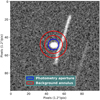 |
Fig. 1 Example of circular aperture photometry on a 10-second observation of EF obtained with the TRAPPIST-North telescope (pixel size of 1.2″/pix). The flux of the target is captured by the first innermost blue aperture, while the gap between the innermost and second aperture is ignored. The pixels between the outermost and second aperture (two red apertures) are used to compute the sky-background level. |
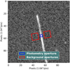 |
Fig. 2 Example of our square apertures on a trailed observation of BX1 (pixel scale of 1.04″/pix) observed at the Schiaparelli Observatory. The blue square aperture centered on the trail is used to capture the asteroid flux. The red square apertures located on both sides of the trail are used to compute the sky-background level. |
2 Aperture photometry on trailed objects
Aperture photometry on trailed observations of fast moving asteroids represents a significant departure from conventional techniques, such as aperture photometry on point-source-like objects. In traditional aperture photometry, circular apertures are typically employed to enclose the target positions in the image and define the background sky brightness, facilitating the measurement of its flux. To perform aperture photometry on trailed observations of asteroids, we use a square or rectangular aperture aligned with the direction of the NEO’s trail (see Fig. 2). This technique maximizes the signal-to-noise ratio of the extracted photometry over a small section of the trail. We then step along the trail to collect the photometry as a function of time. In the following subsections, we go through all the steps that we are taking to go from a trailed image of an asteroid to a fully reduced calibrated light curve.
2.1 Preprocessing
The preprocessing steps include all the typical steps usually performed for photometric analysis of astronomical observations (i.e., bias and flats). The photometric and astrometric calibration of the images is also not fundamentally different from any other regular processing of star or asteroid observations. For this step, we use the photometrypipeline Python package (Mommert 2017). This pipeline automatically extract the sources using sextractor (Bertin & Arnouts 1996) and then solves the plate astrometrically using scamp (Bertin 2006). The sidereally tracked observations allow accurate plate solutions to be obtained using the stars.
What is different is how the photometry of the asteroid is obtained from the trails. For an accurate absolute calibration of the extracted photometry of the asteroid using our technique, it is important to use a large aperture for the photometric calibration of the stars in the background. This is due to the fact that the shape of the PSF for the stars (circular, but convolved with the seeing variation and the motion of the stars due to tracking inaccuracies) and that of the asteroid (elongated in the direction of motion and not affected by long-term seeing variation and tracking errors) are different. The result is that the PSF of the asteroid will be smaller than that of the stars in an unpredictable way.
To address this issue, we need to take apertures large enough to encompass the whole PSF. In practice, this can be done by performing a curve of growth analysis of the zero point (ZP; i.e., the magnitude of an object that would have a flux of 1 on the observed image). As the aperture increases, the ZP magnitude will grow until it reaches a plateau when the aperture becomes large enough to encompass all (or a large fraction of) the light from the stars. An example of such a growth curve is presented in Fig. 3. The ZP will then be estimated by fitting an exponential curve to the curve of growth. Its value corresponds to the limit at high apertures of the fitted curve.
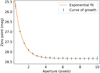 |
Fig. 3 Example of a ZP curve of growth for the last observations of BX1 presented in this work. The ZP magnitude increases with the aperture size until reaching a plateau around 28.53 mag. |
2.2 Determination of the location of the trail
The first step in our new processing routine consists of determining where the asteroid trail is located on the image. This is done by querying the ephemerides of the target using the jplhorizons module from the astroquery python package (for the rest of the paper, every time we query ephemerides this module is used). From the header we extract the time of mid-exposure. We can then estimate the time when the exposure started and stopped according to the total exposure time of the acquisition. By querying the ephemerides for both of these timestamps, we obtain the location in right ascension (RA) and declination (Dec) of the target at the beginning and end of the exposure and thus the location of both ends of the trail. Using the World Coordinate System (WCS) information from the astrometric calibration of the image and using the astropy wcs function (Price-Whelan et al. 2022), we can convert the asteroid RA and Dec into x and y coordinates on the image.
The real start and end of the exposure can be slightly different from the computed ones because of time biases due to errors in the clocks or timing of the shutter opening and closing. Such biases are common in the header of astronomical images (Farnocchia et al. 2023). For such rapidly moving objects, this quickly results in a detectable offset on the image along the direction of the trail. This discrepancy can be easily solved by applying an offset to the queried time. This offset can either be precisely determined by observing GNSS (Global Navigation Satellite System) satellites (Farnocchia et al. 2022) or can be manually applied such that the obtained x and y coordinates correspond best with the beginning and end of the trail.
Another source of random offsets are imperfections in the tracking of the telescope during the exposure. We correct this offset by detecting the location of the beginning and end of the trail by fitting its precise location. For this, we first extract a sub-image centered on the pixel provided by the ephemerides (corrected from the time biases; sub-image (a) in Fig. 4). The image is then rotated to align the trail with the y-axis (sub-image (b) in Fig. 4). The rotation is performed using the rotate function from the skimage transform python package (Van der Walt et al. 2014), and the angle of rotation is determined using the direction of motion of the object from the ephemerides. Even if we do not use this rotated image for photometric purposes, we use the preserve_range option to preserve the fluxes. Once the asteroid trace is aligned with the y-axis, we can reduce the two-dimensional image to a one-dimension line on both axes by taking the sum, median, or mean along the columns or rows. The median of all rows is fitted with a Moffat function (Moffat 1969) to locate the position of the trail (sub-image (d) in Fig. 4), while the sum of all columns is fitted with an erf function to locate where the trail starts (sub-image (c) in Fig. 4). The coordinates obtained through the fitting processes on the rotated images are then de-rotated and converted back to the full image coordinates to locate the position of the trail (sub-image (a) in Fig. 4 on the non-rotated image).
2.3 Stepping along the trail
Once the beginning and end of the trail is precisely located, we compute its length and divide it by the size of the full width at half maximum (FWHM) of the star PSF. The effective exposure time for each aperture can be chosen by the user. However, the optimum value is typically chosen to correspond to aperture sizes approximately equal to the FWHM of the circular star PSF (Mighell 1999, see our Sec. 2.4).
This way we subdivide the trail into pieces with sizes corresponding to the time needed for the object to move over one seeing unit. We then loop through all the epochs, query the ephemerides, convert the RA and Dec into x and y positions, and fit a Moffat function to the trail to correct for imperfections from tracking.
2.4 Aperture size
An optimized aperture size can be obtained by performing a curve of growth for the flux extracted from the trail of the asteroid with different aperture sizes. For each aperture size, the uncertainty on the extracted flux can be estimated using the CCD equation (Howell 2006) that takes into account the total flux inside the aperture, the area of the aperture, the background level, and the area of the aperture used for determining the background level. Here we ignore the contribution from the dark current and the readout noise, which are negligible for modern professional CCD cameras. The optimal aperture size will be the one that minimizes the computed theoretical uncertainties on the extracted flux.
Figure 5 shows an example growth curve of the median of the uncertainties for all the measurements extracted along the trail of the last observations of BX1. We see that the uncertainty first decreases rapidly as a function of the aperture size as we extract more and more flux from the trail. Then the curve goes through a minimum, the uncertainty starts to grow due to the addition of more and more flux from the sky background (noise), and no additional flux from the trail is added anymore (signal). The optimal aperture corresponds to the one that minimizes that curve.
In Fig. 5 we show the size of the median FWHM of the trail, whereby the FWHM is computed by fitting a Moffat function at all positions from which we are extracting flux. We also show the median FWHM of all stars. We see that the optimal aperture is located in between these two values, but the differences in uncertainties between these values is marginal and using the FWHM of the stars is a good default aperture value. Moreover, the decreasing part of the curve is much faster than the growing part. Using a too small aperture will affect the uncertainties more than using a too large aperture. It is thus safer to favor larger apertures over smaller ones.
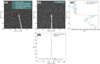 |
Fig. 4 Determination of the location of the trail. (a) Cropped image around one end of the trail. The blue circle (located around the coordinates (60,100)) represents the expected position of the asteroid at the beginning or end of the exposure based on the ephemerides and the time read from the fits header. The orange circle corresponds to the expected position of the asteroid at the beginning or end of the exposure after correcting for the time bias in the header, while the green circle corresponds to the true position of the object after fitting the end of the trail. (b) Same image as (a) but after rotation to align the trail with the y-axis. (c) Sum of the flux after adding pixels along the rows. The blue line is fitted with an error function to locate at which row the trail starts. We note that the variation in the flux of the asteroid due to its rotation is already visible in the blue curve. (d) Median flux integrated along the columns of pixels. The blue line is fitted with a Moffat function to determine in what column the trail is located. |
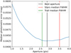 |
Fig. 5 Growth curve of the median of the theoretical uncertainty for all measurements along the trail. The minimum of the curve (represented by the vertical black line) corresponds to the computed optimal aperture (2.8 pixels here). The vertical green line corresponds to the median FWHM of the trail (2.55 pixels), while the vertical red line corresponds to the median FWHM of all the stars in the field (3.5 pixels). |
2.5 Extracting the photometry
To perform aperture photometry on trailed observations of asteroids, we use a square or rectangular aperture aligned with the direction of the NEO’s trail (see Fig. 2). The alignment is done by rotating the aperture according to the direction of motion of the object. This direction can be obtained by querying the ephemerides, wherein the direction of motion is retrieved using the Sky_mot_PA field. The direction of motion can also be obtained by querying ephemerides at two short intervals of time (typically such as the asteroid moves by a few pixels in between these two epochs) and computing the directional vector.
For these fast-moving (close to Earth) objects, the apparent motion in the sky can vary significantly during the exposure. Since we are querying the ephemerides at fixed intervals of time, we need to adjust the size of the apertures to match the relative speed of the objects. It is important to keep a constant effective exposure time (time covered by the aperture) in order to keep identical relative fluxes. So if the extracted flux varies, this is due to intrinsic variations in the object’s brightness and not variation due to the effective exposure time. The final step involves multiplying the observed flux for each individual aperture by the ratio between the total and effective exposure times (time needed for the target to cross the aperture) to obtain calibrated magnitudes for the asteroid observations.
As conventionally used for circular aperture photometry, we estimate the flux of the sky background at an appropriate distance from the observed trailed object. This allow to accurately assess the background flux affecting the source without being contaminated by it. We use the Python package Photutils (Bradley et al. 2023) to generate the rectangular apertures and conduct the photometry. We also utilize the source masking capabilities of Photutils to remove pixels contaminated by background sources within the aperture used to estimate the sky-background flux.
The optimum apertures are square apertures whose sizes are approximately equal to the FWHM computed using the stars (see Sec. 2.4). This both ensures the optimal extraction of the flux perpendicular to the trail (Mighell 1999) and provides the smallest apertures that can be used to obtain independent temporal measurements. Here, for two consecutive measurements, we use apertures that touch each other, but without overlapping, to maximize the flux extraction. This makes consecutive observations slightly correlated with each other. When the target is centered at the limit of two square apertures, half of its PSF will be located in one aperture and the other half in the other aperture. To obtain fully independent observations, gaps of at least one FWHM need to be added between measurements. This can be done simply by removing every second measurement. Alternatively, longer rectangular apertures can be used in the direction of the trail to increase the flux, thus increasing the signal-to-noise ratio of individual measurements at the cost of decreasing the temporal resolution.
It is important to note that the sky must be photometric during the exposure. Any temporal variation in extinction affects the integrated star and asteroid images differently. However, the same issue arises for star-trailed observations.
3 Observations and results
3.1 2023 CX1
Asteroid 2023 CX1, which was temporarily known by its discoverer-assigned identificator Sar2667, was initially spotted by Krisztián Sárneczky, an astronomer at the Konkoly Observatory’s Piszkéstető Station (MPC code 461) in Hungary. This observation was obtained on 2023 February 12 at 20:18 UT and quickly triggered impacting alerts from the NASA and ESA impact monitoring services Scout2 and Meerkat (Frühauf et al. 2021). Six hours after its discovery, CX1 impacted on 2023 February 13 at 02:59 UT, over the coast of Normandy in France. This event marked the seventh time a small asteroid had been discovered before impacting Earth. By combining the precise knowledge of its trajectory as it entered the atmosphere with atmospheric wind data and the observed fragmentation altitude from fireball observations in the FRIPON meteor monitoring network (Colas et al. 2020), meteorites were recovered on the ground (Jenniskens & Colas 2023). This was only the third time that meteorites were recovered from an asteroid discovered prior to impacting Earth (Jenniskens et al. 2009, 2021).
At the time of its discovery, the object was already within 233 000 km of Earth and moving at a speed of 0.19″/s on the plane of the sky. Over the next six hours, its speed gradually increased, reaching more than 1000″/s just before entering the Earth shadow and impacting. With an estimated absolute H magnitude of 32.7, its size is calculated to range between 0.8 and 1.7 m.
We analyzed four trailed observations of CX1 obtained at the Schiaparelli Observatory located in northern Italy, atop mount Campo dei Fiori near Varese, 1230 m above sea level (MPC 204). A 0.84 m Newtonian telescope was used with an SBIG STX-16803 camera, which provides a field of view of 42′ × 42′ with a pixel size of 1.87″ when operated in 3 × 3 binning mode. The observations were unfiltered, with an exposure time of 60 s.
The first observation was obtained at 02:29 UT, when CX1 was moving at a speed of ~2.45″/s (the speed varied significantly over the time span of the exposure) and thus trailed over 76 pixels. The last image was obtained at 02:50 UT, only 9 min before impact, when CX1 was located at 7000 km from the observer (varying between 7575 km and 6877 km during the 60 s of the exposure). At that time, it was moving at a speed of more than 15″/s and trailing over 441 pixels. The rapid change in distance to the asteroid and the relative motion in the sky caused the trail to curve significantly, as can be seen in Fig. 6. Information on all individual exposures can be found in Table 1.
The CX1 photometric observations are presented in Fig. 7, with each color representing a different trail. The magnitude was calibrated in the V band independently for each acquisition using the field stars. The time is expressed in minutes before the impact. The rapid brightening of CX1 is clearly visible as it approaches Earth.
We searched for the signature of rotation in the asteroid photometry by folding all data into a phase curve according to trial spin periods. To avoid any effect from the correlation between consecutive measurements in the period search, we considered only every other measurement. This reduces the number of total measurements by a factor of two but assures that they are all independent of each other. For each period, a Fourier series of order 5 was fitted and the chi-square of the fit to the data was computed to create a periodogram. The phase curve is expected to have two minima for one rotation but can be more complicated if the object is tumbling. Figure 8 shows the periodogram of CX1 for periods between 0.36 seconds and 6 minutes. The periodogram exhibits several chi-square minima.
Figure 8 shows two attempts to fold the data according to the two strongest minima. A period of 9.16 s (left diagram) does not show the expected double minimum in the phased light curve, which may represent just half a spin period. A period of 18.33 s does result in the expected double minimum, but the amplitude is small, leading to a poor significance level; this is most likely just due to noise rather than the asteroid rotation.
The photometric accuracy is approximately 0.1 mag, with an effective exposure time around 0.25 s. In this case, the asteroid was nearly spherical in shape, was observed close to a pole-on geometry, or had a period much longer than 6 min, resulting in a light curve amplitude smaller than 0.1 mag.
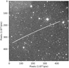 |
Fig. 6 Trailed observation of CX1 obtained at the Schiaparelli Observatory nine minutes before impact (pixel scale of 1.87″/pix). The exposure time was 60 seconds, during which CX1 trailed over 441 pixels. The curvature of CX1’s trail is attributed to its very close proximity to the observer (approximately 7000 km) and the rapid variation in its relative motion in the sky. |
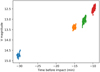 |
Fig. 7 CX1 photometry derived from four trailed images. Each color represents a different image of 60 s each. The x-axis gives the time in minutes before the impact time, while the y-axis is the V magnitude. |
3.2 2024 BX1
2024 BX1, temporarily named Sar2736 by the discoverer, is the third impactor asteroid discovered by Krisztián Sárneczky at Hungary’s Konkoly Observatory’s Piszkéstető Station (MPC code 461). The discovery occurred just three hours prior to its impact on Earth, leaving little time for its physical characterization. Meteorites were recovered on the ground (Jenniskens et al. 2024b). We analyzed trailed observations of BX1 obtained at the Schiaparelli Observatory. Like CX1, BX1 displayed the same H magnitude of 32.7, leading to the same estimated size of 0.8-1.7 m. Analysis of the fireball light curve suggests a smaller size of 0.44 m, probably because the aubrite meteorites recovered on the ground have an unusually high albedo (Jenniskens et al. 2024a; Spurnỳ et al. 2024).
The telescope used was the same as that used for CX1, but with a QHY600M CMOS camera instead of the SBIG STX-16803. The QHY600M offers a 41.6′ × 27.8′ field of view with a pixel scale of 1.04″ when used in a 4-by-4 binning mode. The first observations were obtained when the asteroid was located at a distance of 17 500 km from Earth and moving at a speed of 7.6″/s. The last observations were obtained just 11 minutes before impact at a distance of 9500 km from the observer, at which time the asteroid was moving at a speed of more than 30″/s. Information about all the individual observations can be found in Table 1.
Contrary to CX1, we find a clear rotational signature with a period of P = 2.5888 ± 0.0002 s and a light curve amplitude of 0.7 mag (Fig. 9). As for CX1, only one of every two measurements was considered to avoid bias effects from the measurements being correlated. All photometric observations, calibrated in the V band independently for each acquisition using field stars, are combined in Fig. 10, where the x-axis represents the time before impact. As for CX1, we see a clear brightening of the object as it approached Earth. Figure 9 shows the periodogram for test periods between 0.36 and 7.2 s. There is an evident signal at a period of P = 2.5888 ± 0.0002 s, along with its aliases (varying numbers of maxima and minima).
This is the fastest rotation period ever measured for an asteroid. It is 13% faster than the previous record held by 2020 HS7, which had a rotation period of P = 2.99 s (Beniyama et al. 2022). Analysis of the signification of such a fast rotation is beyond the scope of this paper and is left to other work.
3.3 2024 EF
The trailed imaging technique is not limited to Earth impactors; it is also relevant for somewhat larger asteroids. The asteroid EF performed a close fly-by with Earth at a minimal distance of 57 614.5 ± 2.4 km on 2024 March 4, less than 48 hours after its discovery on March 2. With an estimated H magnitude of 29, the size is in the range 4 to 10 m.
We observed EF with the TRAPPIST-North telescope located at the Oukaimaiden Observatory in Morocco (TN; MPC Z53). TRAPPIST-North is a robotic telescope that uses a 0.6 m Ritchey-Chrétien design operating at f/8 on a German Equatorial mount. It is a clone of TRAPPIST-South, which is located at La Silla Observatory in Chile (Jehin et al. 2011). The camera is an Andor IKONL BEX2 DD (0.60″/pixel, 20′ × 20′ field of view). Images were obtained with a binning of 2×2 and a blue cutting filter with transmission starting at 500 nm.
We performed both “regular” observations (with tracking on the asteroid motion) and trailed observations. The regular observations had exposure times of 20, 10, and 3 s. The stars were trailing over several dozen pixels, preventing us from using them for photometric calibration (see Fig. 1). However, typical circular aperture photometry allowed us to determine a rotation period of 3.95 min for this object using the latest and shortest exposure time observations (3 s).
We also analyzed one trailed acquisition that lasted 90 s using our technique. Although this acquisition is much shorter than the known rotation period, we were able to observe a trend in the photometry that could be phased with the light curve obtained just before and after. Figure 11 shows the trailed observation analysis in blue squares. The photometry obtained just before and after using regular asteroid-tracked observations are shown in orange. We utilized the orange observations to search for the best Fourier series fit, represented by the continuous black line. We can see that the trailed observation fits nicely to the trend obtained with the orange observations only. The trailed observations have been binned 15 times to better align with the exposure times of the regular observations and to enhance visibility on the plot.
Additionally, we note that there is a hint that EF is in a tumbling state, because the amplitude of the light curve changes over time following a regular decrease and increase. Because of that, we were not able to perfectly phase all the observations (which spanned several hours) using the 3.95 min period. While short sections can be phased without issue, we again notice a departure from perfect phasing in Fig. 12, where each individual rotation is displayed using a different color. We do not report the uncertainty on this period as this would require a more detailed analysis of the tumbling nature of the rotation state and is beyond the scope of this paper.
All trailed observations analyzed in this work.
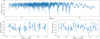 |
Fig. 8 Results of the period search for CX1. Upper plot: periodogram for all the observations of CX1, testing periods between 0.36 s and 6 min. Bottom plots: observations phased according to the two best test periods. We do not find any convincing solution for the rotation period of CX1, although the solutions at P=9.16 s (left) and 18.33 s (right) are plausible. |
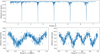 |
Fig. 9 Results of the period search for BX1. Upper plot: periodogram of all the observations of BX1 testing periods between 0.36 and 7.2 s. We see a clear minimum at 2.5888 s and its aliases. Bottom: observations phased according to the two best results, 2.5888 and 5.1775 s. |
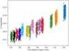 |
Fig. 10 Photometry of BX1 derived from all trailed images. Each color represents a different image of 30 s each. The x-axis gives the time in minutes before the impact time, while the y-axis is the magnitude in the V band. |
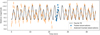 |
Fig. 11 Light curve of asteroid EF obtained with TRAPPIST-North from 02:43 UT to 03:33 UT on 2024 February 4. The orange dots correspond to regular asteroid-tracked observations, and the blue squares correspond to the photometry derived from one single trailed observation of 90 s. The black curve corresponds to the best Fourier fit on the orange observations only. |
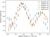 |
Fig. 12 Phased light curve of EF assuming a period of 3.95 min. |
4 Discussions
The new method of aperture photometry for fast-moving asteroids has limitations and is not meant to replace all traditional aperture photometry. However, it can be extremely useful when certain conditions are met. In this section we discuss the pros and cons of the new method and when an observer should decide to perform asteroid observations tracked on the stars or on the asteroid.
4.1 CCD or CMOS camera
The main advantage of this new method is its ability to extract the timing information on a scale much smaller than the typical CCD readout time. As we saw for BX1 earlier in this paper, small asteroids can have rotation periods smaller than the typical readout time of traditional CCDs. However, fast readout CMOS cameras are becoming more and more common. If the available camera has a readout time much shorter than the quickest expected rotation period for an object, then more accurate photometric observations can be obtained by keeping the exposure time short and the asteroid at a fixed position on the sensor.
4.2 Asteroid size
The expected rotation period of an asteroid is directly dependent on its size (i.e., its H magnitude). An analysis of the allowed rotation period as a function of the asteroid size is beyond the scope of this paper, but according to the Near-Earth Observations Coordination Center (NEOCC) physical properties web portal3, at the time of writing this paper, no object with an H magnitude brighter than 24 displays a rotation period faster than 60 s. Hence, if the observed object is large (H<24), traditional observation techniques would be more effective than the one presented in this paper.
4.3 Asteroid sky motion speed
The method presented in this work should only be used for asteroids that display rapid angular motion on the plane of the sky. Whether an observer should use regular observations or trailed observations will depend on each individual telescope and camera setup and the sky conditions (seeing, field of view, readout time of the CCD, telescope size, etc.). If the asteroid motion is slow enough to not move by more than one FWHM in less than the readout time of the camera used to obtain the observations, using a conventional observation method will be more effective than using trailed observations. If the asteroid is moving too fast, the signal-to-noise ratio of each individual measurement along the trail will be too low and thus regular observations techniques should also be used.
4.4 Close fly-by of newly discovered objects
Just after an asteroid is discovered, its orbit will be poorly known. Usually, follow-up observations will improve our knowledge of the orbit. As long as the location and speed of the object is poorly known, the positional uncertainties are usually greater in the direction of motion of the object than the direction perpendicular to it. When asteroids move fast on the sky, the most optimum strategy is thus to pre-point the telescope where the object will be located in the near future, start a series of trailed exposures, and wait for it to cross the field of view. These initial uncertainties in the ephemerides are irrelevant for the data reduction as it can be performed after the fly-by. Updated information on the orbit will thus be available, allowing for precise times and locations to be obtained for the object in the image.
4.5 Goal of the observation
While small asteroids in a close fly-by can be bright, we saw in our discussion of the method that letting the asteroid trail on the image resulted in the PSF of the stars and the asteroid being different. This could lead to issues in the absolute calibration of the magnitude of the object. Moreover, if the field of view cannot be properly flat-fielded, the fact that the object is moving through a large fraction of the CCD can lead to biases in the photometry. This is not an issue if the observer is interested in deriving the rotation period of the object. However, if the goal of the observation is to derive the phase curve, a high precision on the absolute calibration of the photometry is needed, and regular observation methods would be more effective.
5 Conclusions
We present in this paper a novel approach to performing photometry of fast-moving near-Earth asteroids. Instead of tracking the asteroid motion, which leads to stars appearing trailed on the images, we observe the asteroid using sidereal tracking and let the asteroid sweep through the field. This results in the asteroid appearing trailed on the images.
The advantage of this technique is that it allows the brightness of the object to be extracted over time in single images by extracting the photometry using square apertures at different locations on the trail. We show that this technique works and is highly effective in detecting fast-rotating asteroids for which usual observation techniques would have failed to retrieve the period because their overhead time (readout time of the CCD) is longer than the rotation period of the asteroid.
We analyzed three recently observed rapidly moving asteroids, CX1, BX1, and EF. The first two impacted Earth a few minutes after our observations ended, while the third one made a close fly-by.
For CX1, the photometric variation is less than 0.1 mag. This suggests that the object is shaped nearly like a sphere, was seen pole-on, or did not rotate much during the span of our observations.
In the case of BX1, we observed the fastest rotation period ever measured for an asteroid: P = 2.5888 ± 0.0002 s. In this case, the asteroid was elongated, resulting in a large amplitude variation in brightness.
In the case of EF, we observed a rotation period of approximately 3.95 min using regular asteroid-tracked observations. However, we show that the photometry extracted on a single 90 s exposed trailed image can be correctly phased with the regular observations.
Based on these results, we encourage observers to obtain trailed observations of asteroids when:
The asteroid motion on the sky is so fast that the exposure time would be significantly shorter than the CCD readout time (to maximize the observation time).
The asteroid is small, with an H magnitude brighter than 24 (the asteroid could be a rapid rotator).
The asteroid was recently discovered and has imperfect ephemerides (the observers should avoid having both trailed star and trailed asteroid images).
The observer does not need high accuracy for the absolute magnitude (i.e., their interest is instead focused on determining the rotation state of the object).
In any other circumstance, the use of regular observation techniques should be favored. However, we encourage observers to regularly take a few trailed observations, alongside regular observations, as a single 30–60 s observation could allow the determination of the rotation period or at least help in breaking alias issues for fast-rotating objects.
The use of trailed observations allowed us to obtain the fastest rotation period known to date. However, asteroids are expected to rotate even faster. The limitation in detecting fast rotation periods arises from the use of exposure times longer than the rotation period. Fast-spinning asteroids are expected to be small and thus faint when located far from Earth. It is thus important to take advantage of their impacting and very close fly-by events to obtain reliable physical characterizations for them.
Acknowledgements
This research made use of Photutils, an Astropy package for detection and photometry of astronomical sources Bradley et al. (2023). TRAPPIST-North is a project funded by the University of Liège, in collaboration with the Cadi Ayyad University of Marrakech (Morocco) and the Belgian Fund for Scientific Research (FNRS) under the grant PDR T.0120.21. E. Jehin is a FNRS Research Director. This work made use of the NASA JPL Horizons ephemerides service available at https://ssd.jpl.nasa.gov/horizons/ PJ is supported by NASA’s YORPD program (grant NNH21ZDA001N).
References
- Beniyama, J., Sako, S., Ohsawa, R., et al. 2022, PASJ, 74, 877 [NASA ADS] [CrossRef] [Google Scholar]
- Bertin, E. 2006, ASP Conf. Ser., 351, 112 [NASA ADS] [Google Scholar]
- Bertin, E., & Arnouts, S. 1996, A&AS, 117, 393 [NASA ADS] [CrossRef] [EDP Sciences] [Google Scholar]
- Bolin, B., Ghosal, M., & Jedicke, R. 2024, MNRAS, 527, 1633 [Google Scholar]
- Bradley, L., Sipőcz, B., Robitaille, T., et al. 2023, https://doi.org/10.5281/zenodo.7946442 [Google Scholar]
- Colas, F., Zanda, B., Bouley, S., et al. 2020, A&A, 644, A53 [EDP Sciences] [Google Scholar]
- Farnocchia, D., Reddy, V., Bauer, J. M., et al. 2022, PSJ, 3, 156 [NASA ADS] [Google Scholar]
- Farnocchia, D., Reddy, V., Bauer, J. M., et al. 2023, PSJ, 4, 203 [Google Scholar]
- Frühauf, M., Micheli, M., Oliviero, D., & Koschny, D. 2021, in 7th IAA Planetary Defense Conference, 97 [Google Scholar]
- Howell, S. B. 1989, PASP, 101, 616 [CrossRef] [Google Scholar]
- Howell, S. B. 2006, Handbook of CCD Astronomy, 5 (Cambridge: Cambridge University Press) [Google Scholar]
- Jehin, E., Gillon, M., Queloz, D., et al. 2011, The Messenger, 145, 2 [NASA ADS] [Google Scholar]
- Jenniskens, P., & Colas, F. 2023, CBAT, 5230, 613 [Google Scholar]
- Jenniskens, P. a., Shaddad, M. H., Numan, D., et al. 2009, Nature, 458, 485 [NASA ADS] [CrossRef] [Google Scholar]
- Jenniskens, P., Gabadirwe, M., Yin, Q.-Z., et al. 2021, Meteor. Planet. Sci., 56, 844 [NASA ADS] [CrossRef] [Google Scholar]
- Jenniskens, P., Hecht, L., Greshake, A., Helbert, J., & Hamann, C. 2024a, Meteor. Bull., 113 [Google Scholar]
- Jenniskens, P., Hecht, L., Hamann, C., Greshake, A., & Helbert, J. 2024b, CBAT, 618, 5343 [Google Scholar]
- Mighell, K. 1999, ASP Conf. Ser. 189, 50 [NASA ADS] [Google Scholar]
- Moffat, A. 1969, A&A, 3, 455 [Google Scholar]
- Mommert, M. 2017, Astron. Comput., 18, 47 [NASA ADS] [CrossRef] [Google Scholar]
- Price-Whelan, A. M., Lim, P. L., Earl, N., et al. 2022, ApJ, 935, 167 [NASA ADS] [CrossRef] [Google Scholar]
- Spurnỳ, P., Borovička, J., Shrbenỳ, L., Hankey, M., & Neubert, R. 2024, A&A, 686, A67 [CrossRef] [EDP Sciences] [Google Scholar]
- Thirouin, A., Moskovitz, N., Binzel, R., et al. 2016, AJ, 152, 163 [NASA ADS] [CrossRef] [Google Scholar]
- Thirouin, A., Moskovitz, N. A., Binzel, R. P., et al. 2018, ApJS, 239, 4 [NASA ADS] [CrossRef] [Google Scholar]
- Van der Walt, S., Schönberger, J. L., Nunez-Iglesias, J., et al. 2014, PeerJ, 2, e453 [Google Scholar]
- Vereš, P., Jedicke, R., Denneau, L., et al. 2012, PASP, 124, 1197 [CrossRef] [Google Scholar]
All Tables
All Figures
|
Fig. 1 Example of circular aperture photometry on a 10-second observation of EF obtained with the TRAPPIST-North telescope (pixel size of 1.2″/pix). The flux of the target is captured by the first innermost blue aperture, while the gap between the innermost and second aperture is ignored. The pixels between the outermost and second aperture (two red apertures) are used to compute the sky-background level. |
| In the text | |
|
Fig. 2 Example of our square apertures on a trailed observation of BX1 (pixel scale of 1.04″/pix) observed at the Schiaparelli Observatory. The blue square aperture centered on the trail is used to capture the asteroid flux. The red square apertures located on both sides of the trail are used to compute the sky-background level. |
| In the text | |
|
Fig. 3 Example of a ZP curve of growth for the last observations of BX1 presented in this work. The ZP magnitude increases with the aperture size until reaching a plateau around 28.53 mag. |
| In the text | |
|
Fig. 4 Determination of the location of the trail. (a) Cropped image around one end of the trail. The blue circle (located around the coordinates (60,100)) represents the expected position of the asteroid at the beginning or end of the exposure based on the ephemerides and the time read from the fits header. The orange circle corresponds to the expected position of the asteroid at the beginning or end of the exposure after correcting for the time bias in the header, while the green circle corresponds to the true position of the object after fitting the end of the trail. (b) Same image as (a) but after rotation to align the trail with the y-axis. (c) Sum of the flux after adding pixels along the rows. The blue line is fitted with an error function to locate at which row the trail starts. We note that the variation in the flux of the asteroid due to its rotation is already visible in the blue curve. (d) Median flux integrated along the columns of pixels. The blue line is fitted with a Moffat function to determine in what column the trail is located. |
| In the text | |
|
Fig. 5 Growth curve of the median of the theoretical uncertainty for all measurements along the trail. The minimum of the curve (represented by the vertical black line) corresponds to the computed optimal aperture (2.8 pixels here). The vertical green line corresponds to the median FWHM of the trail (2.55 pixels), while the vertical red line corresponds to the median FWHM of all the stars in the field (3.5 pixels). |
| In the text | |
|
Fig. 6 Trailed observation of CX1 obtained at the Schiaparelli Observatory nine minutes before impact (pixel scale of 1.87″/pix). The exposure time was 60 seconds, during which CX1 trailed over 441 pixels. The curvature of CX1’s trail is attributed to its very close proximity to the observer (approximately 7000 km) and the rapid variation in its relative motion in the sky. |
| In the text | |
|
Fig. 7 CX1 photometry derived from four trailed images. Each color represents a different image of 60 s each. The x-axis gives the time in minutes before the impact time, while the y-axis is the V magnitude. |
| In the text | |
|
Fig. 8 Results of the period search for CX1. Upper plot: periodogram for all the observations of CX1, testing periods between 0.36 s and 6 min. Bottom plots: observations phased according to the two best test periods. We do not find any convincing solution for the rotation period of CX1, although the solutions at P=9.16 s (left) and 18.33 s (right) are plausible. |
| In the text | |
|
Fig. 9 Results of the period search for BX1. Upper plot: periodogram of all the observations of BX1 testing periods between 0.36 and 7.2 s. We see a clear minimum at 2.5888 s and its aliases. Bottom: observations phased according to the two best results, 2.5888 and 5.1775 s. |
| In the text | |
|
Fig. 10 Photometry of BX1 derived from all trailed images. Each color represents a different image of 30 s each. The x-axis gives the time in minutes before the impact time, while the y-axis is the magnitude in the V band. |
| In the text | |
|
Fig. 11 Light curve of asteroid EF obtained with TRAPPIST-North from 02:43 UT to 03:33 UT on 2024 February 4. The orange dots correspond to regular asteroid-tracked observations, and the blue squares correspond to the photometry derived from one single trailed observation of 90 s. The black curve corresponds to the best Fourier fit on the orange observations only. |
| In the text | |
|
Fig. 12 Phased light curve of EF assuming a period of 3.95 min. |
| In the text | |
Current usage metrics show cumulative count of Article Views (full-text article views including HTML views, PDF and ePub downloads, according to the available data) and Abstracts Views on Vision4Press platform.
Data correspond to usage on the plateform after 2015. The current usage metrics is available 48-96 hours after online publication and is updated daily on week days.
Initial download of the metrics may take a while.