| Issue |
A&A
Volume 689, September 2024
|
|
|---|---|---|
| Article Number | A137 | |
| Number of page(s) | 14 | |
| Section | Astrophysical processes | |
| DOI | https://doi.org/10.1051/0004-6361/202450103 | |
| Published online | 09 September 2024 | |
Synchrotron polarization with a partially random magnetic field: General approach and application to X-ray polarization from supernova remnants
1
INAF – Osservatorio Astrofisico di Arcetri, Largo E. Fermi 5, 50125 Firenze, Italy
2
INAF – Osservatorio Astronomico di Palermo, Piazza del Parlamento 1, 90134 Palermo, Italy
e-mail: This email address is being protected from spambots. You need JavaScript enabled to view it.
3
Institute for Applied Problems in Mechanics and Mathematics, National Academy of Sciences of Ukraine, Naukova St. 3-b, 79060 Lviv, Ukraine
Received:
23
March
2024
Accepted:
22
May
2024
Abstract
Context. Diagnostics based on the polarization properties of the synchrotron emission can provide precious information on both the ordered structure and the random level of the magnetic field. While this issue has already been analyzed in the radio band, the polarization data recently obtained by the mission IXPE have shown the need to extend this analysis to the X-ray band.
Aims. While our immediate targets are young supernova remnants, the scope of this analysis is wider. Our aim is to extend the analysis to particle energy distributions more complex than a power law, and to investigate a wider range of cases involving a composition of ordered and random magnetic fields.
Methods. Since an analytical approach is only possible in a limited number of cases, we devised for this purpose an optimized numerical scheme, and we directly used it to investigate particle energy distributions in the form of a power law with an exponential or super-exponential cutoff. We also considered a general combination of an ordered field plus an anisotropic random component.
Results. We show that the previously derived analytic formulae, valid for power-law distributions, may also be good approximations of the polarization degree in the more general case with a cutoff, as typically seen in X-rays. We explicitly analyzed the young supernova remnants SN 1006, Tycho, and Cas A. In particular, for SN 1006 we proved the consistency between the radio and X-ray polarization degrees, favoring the case of a predominantly random field with an anisotropic distribution. In addition, for the power-law case we investigated the effect of a compression on ordered and on random magnetic field components, aimed at describing the mid-age radio supernova remnants.
Conclusions. This work allows a more efficient exploitation of radio and X-ray measurements of the synchrotron polarization, and is addressed to present observations with IXPE and to future projects.
Key words: acceleration of particles / magnetic fields / polarization / radiation mechanisms: non-thermal / ISM: supernova remnants
Corresponding author; This email address is being protected from spambots. You need JavaScript enabled to view it. .
© The Authors 2024
 Open Access article, published by EDP Sciences, under the terms of the Creative Commons Attribution License (https://creativecommons.org/licenses/by/4.0), which permits unrestricted use, distribution, and reproduction in any medium, provided the original work is properly cited.
This article is published in open access under the Subscribe to Open model. This email address is being protected from spambots. You need JavaScript enabled to view it. to support open access publication.
1. Introduction
Relativistic particles spiraling in a background magnetic field (MF) emit synchrotron radiation. In the presence of a homogeneous MF, this radiation is characterized by a very high polarization degree (Π). However, homogeneous fields rarely occur in real cases. In the majority of cases, instead, fields can be disordered to some extent; in addition, large-scale structures may cause a mix of different MF conditions along the line of sight, and even limitations in the instrumental angular resolution may have a superposition of differently oriented MFs as an effect.
From the analysis of observations of synchrotron emission we can derive some properties of the MF and the energy distribution of relativistic particles. In the presence of an inhomogeneous MF, a more careful modeling is required for this derivation, and this is the primary goal of the present work. Here we mainly focus on the case of supernova remnants (SNRs), but many of the results presented can also be applied to other sources.
In a previous paper (Bandiera & Petruk 2016, hereafter Paper I), we thoroughly discussed the behavior of the synchrotron emission and of its Π, in the presence of a MF in which a homogeneous component is (vectorially) combined with a random component, while the relativistic particles are assumed to be described by a power-law energy distribution. This study led to analytic, although rather complex, formulae that apply for instance to the case of radio emission from SNRs, where the synchrotron emission is usually very well approximated by a power law. In particular, we used that approach to analyze the general properties of polarization images of Sedov SNRs in a uniform interstellar medium (Petruk et al. 2017).
The observational possibilities have been extended dramatically with the launch of the IXPE mission (see, e.g., Weisskopf 2022), which for the first time has provided good quality X-ray polarization maps of several sources. In the case of Pulsar Wind Nebulae the X-ray spectra are also power laws, so that our original results can be safely applied, as actually done for the Crab Nebula (Bucciantini et al. 2023), Vela (Liu et al. 2023), and G0.13–0.11 (Churazov et al. 2024). Instead, synchrotron X-ray spectra of shell-type SNRs are characterized by a cutoff. Our formulae have also been used to discuss the polarization degrees in Cas A, Tycho SNR, and SN 1006 (Ferrazzoli et al. 2023; Zhou et al. 2023), but without an extension of our theoretical treatment to spectra with a cutoff the level of accuracy of those estimates could not be assessed.
While an exact analytic treatment to the more general problem seems to be impossible, we devised a new numerical treatment that allows us to extend the analysis of Paper I and to treat with a high level of accuracy cases in which the particle distribution is more complex than a power law.
The plan of the paper is as follows. In Sect. 2 we review some basic concepts from Paper I, and describe the numerical approach we have developed; Sections 2.1 and 2.2 consider, respectively, the case of an isotropic random MF combined with a homogeneous MF, and that of a purely random anisotropic MF, and for each of them show the results for particle distributions well described by a power law times an exponential or super-exponential cutoff. In Sect. 3 we apply our techniques to observable quantities such as the polarization degree, the spectral index, the spectral curvature, and we discuss the relations between them and with the properties of the emitting system. We also discuss with what level of accuracy our analytic formulae from Paper I (derived for the power-law electron spectrum) could be used in a more general case of particle distribution with a high-energy cutoff. In Sect. 4 we discuss some young SNRs, and in particular SN 1006, for which the mapping of the polarization degree in X-rays with IXPE is particularly detailed and allows a close comparison with the polarization in radio. In Sect. 5 we investigate the case of the ordered plus anisotropic random MF components. We conclude in Sect. 6.
2. The method of calculation
We first review some basic formulae of the classical theory of the synchrotron emission. As a reference for the formulae and notation we used the book by Rybicki & Lightman (1986).
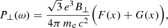
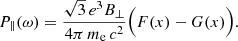
We consider the average emission from a single particle with a given Lorentz factor γ. In this case, the synchrotron power emitted per unit frequency1 can be computed as the sum of two polarized components, respectively perpendicular (P⊥) and parallel (P∥) to the direction of the projected MF (labeled B⊥, being perpendicular to the line of sight, LoS):
 (1)
(1)
 (2)
(2)
Here
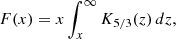 (3)
(3)
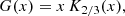 (4)
(4)
with Kn(z) being a modified Bessel function of the second kind, while the variable x is defined as
 (5)
(5)
(which represents a definition for K), where ωc is called the critical frequency.
We first consider an orientation of the local axes (namely in the volume element under consideration) such that the unit vector  is perpendicular to B⊥, while
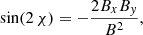
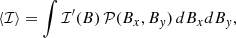
  is parallel to it. With respect to these axes, the Stokes parameters ℐ′ (total flux) and 𝒬′ (linear polarization) read
 (6)
(6)
 (7)
(7)
while the other two Stokes parameters are vanishing: 𝒰′ due to the chosen orientation of axes, 𝒱′ due to the properties of the synchrotron radiation. In the following, while still considering the MF perpendicular to the LoS, we no longer use the symbol B⊥, but simply B (but still having in mind that it is a 2D vector).
We also introduce a fixed reference coordinate system, x–y, which in the following we refer to as the “observer’s coordinate system”. We now represent B as the composition of the homogeneous MF  that, without loss of generality, we assume directed along the y-axis, and of a random MF. We denote as Bx and By the components of the combined field in the observer’s coordinate system, and ℐ, 𝒬, and 𝒰 are the Stokes parameters in this system. In the case of a symmetric distribution for the random MF we expect to have 𝒰 = 0.
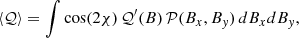
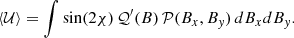
The x′–y′ coordinate system “wiggles” all the time, so that in order to derive time-averaged quantities we always have to account for a rotation on a suitable angle χ to recover the same orientation of the fixed x–y coordinate system. This rotation has no effect on ℐ (ℐ = ℐ′), while the Stokes parameters 𝒬 and 𝒰 transform according to 𝒬 = cos(2 χ) 𝒬′ and 𝒰 = sin(2 χ) 𝒬′, where
 (8)
(8)
 (9)
(9)
and the angle χ between the axis y and the vector B is measured counter-clockwise by the observer2. With the use of the above formulae, in Paper I we first integrated the Stokes parameters over the probability distribution of the random MF components. For this, we explicitly considered two cases: a homogeneneous field plus an isotropic random component, and an anisotropic random MF plus a negligible homogeneous MF.
A clarification is needed about this point. By using this approach, namely by integrating over a probability distribution for the random MF, we implicitly assume that virtually all possible realizations are reached, with frequencies very close to their assigned probabilities. In principle, this is only valid for infinite systems. On the contrary, in the case of only a few realizations along the LoS, our method gives only the statistical average, while in the various cases, taken individually, one could measure a more or less relevant dispersion of values. Such a dispersion may be relevant in the case of a developed turbulence with an injection length scale comparable with the length of the LoS, while it should be negligible in the case of an injection length scale much smaller than the LoS.
The treatment of real turbulence is beyond the scope of the present work, and it will be discussed in a forthcoming paper. Here we limit our description to a random MF, namely fully characterized by its probability distribution function. Our results will also hold in the case of a finite although rather large number of statistically independent cells along the LoS. In this case, the size of cells that could possibly create measurable effects is so large that the MF conditions in them are frozen during the time of observation, while the only effect of a finite exposition time is to account for the uncertainties during the model fitting. The longest exposure times, with IXPE, do not exceed one month, while random motions should be much slower than 1000 km/s. Even in this very extreme case, the size of a cell in which magnetic field changes during an observation run should be smaller than 10−4 pc (compared to a SNR size of ∼1 pc); in addition, in the case of real turbulence the power spectrum of the velocity fluctuations is smaller at smaller scales. Moreover, in the case of lower instrumental resolution the contributions of different LoSs will add up, so that the effective number of the independent cells will be even larger, and consequently the level of possible fluctuations around the mean value in the distribution function will be even smaller.
In a second stage, we then integrated over the particles energy distribution, a power law in that case. Thanks to simplifications for the special case of a power-law distribution, in Paper I we obtained analytic formulae, although involving special functions.
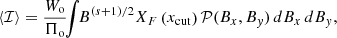
By releasing the condition of a power-law particle distribution, the problem becomes much more complex, so that analytic formulae can no longer be obtained. For this reason a numerical approach is required, but we took maximum advantage of some analytical results to speed up the computations dramatically. In this new approach we found it more convenient to proceed in the opposite order with respect to Paper I, by performing first the integration over the particle distribution, while later on the average over the MF fluctuations. We considered the following family of particle energy distributions
 (10)
(10)
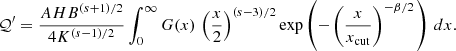
with positive s and β; γcut indicates the position of the cutoff in the particle energy distribution. Therefore, for ℐ′ integrated over the energy distribution, we can write
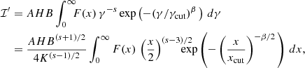 (11)
(11)
where
 (12)
(12)
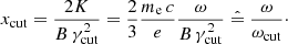
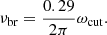
By recalling that the peak of synchrotron emission for a given Lorentz factor is at ω = 0.29 ωc (this quantity is also conventionally adopted in the monochromatic approximation of the synchrotron emission), in order to conform to this standard approach let us define the break frequency as
 (13)
(13)
In a similar way to what was obtained for ℐ′, we also get
 (14)
(14)
In the pure power-law case, the standard result is recovered
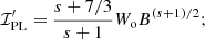 (15)
(15)
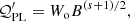 (16)
(16)
where
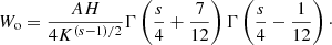 (17)
(17)
With the more general form of energy distribution, as from Eq. (10), a new numerical calculation must be performed for any choice of s and β. It is already rather complex in the case of a homogeneous MF, but it becomes excessively heavy when a random MF component is also present. A brute force approach to this problem would involve the calculation of many random instances for the MF, according to a given distribution function of the random MF component, and then to average among all these cases. For each actualization of the Bx and By field components, we must first derive the total MF B, after which we compute the quantities ℐ′ (equal to ℐ) and 𝒬′ with the use of Eqs. (11) and (14) (which is the most cumbersome part because it involves the calculation of rather heavy integrals), and then we obtain 𝒬 and 𝒰 with the use of Eqs. (8) and (9).
The Stokes parameters are finally obtained as the averages over all these instances. Unfortunately, this approach converges rather slowly, due to the fact that the uncertainty on the average is proportional to the inverse square root of the number of cases used. However, there is a way to significantly speed up the calculations without any substantial loss of accuracy. We note that the formulae for ℐ′ and 𝒬′, the quantities whose evaluation absorbs most of the time, do not depend on both Bx and By, but only on the MF module B. So, an array of their values could be computed first, and then interpolations could be used for each actualization of the MF.
For a given probability distribution 𝒫(Bx, By) of the components of the total (transverse) MF B, the average Stokes parameters are then evaluated in the observer’s frame as
 (18)
(18)
 (19)
(19)
 (20)
(20)
We note that the formulae above assume only variations of the MF, without changes in the density of the emitting particles. Assuming a symmetric distribution 𝒫(Bx, By) with respect to Bx, the quantity ⟨𝒰⟩ vanishes, and the polarization degree is Π = ⟨𝒬⟩/⟨ℐ⟩. We may introduce the functions  and
and  :
:
 (21)
(21)
 (22)
(22)
For a given choice of s and β, the quantities XF and XG are functions of xcut only. In addition, both functions, defined in this way, approach asymptotically 1 for xcut → 0 (see Appendix B for more details). Therefore, the above formulae translate into
 (23)
(23)
 (24)
(24)
where
 (25)
(25)
is the polarization degree for a homogeneous MF.
We now assume that the components of the total (transverse) MF B are well described by a Gaussian probability distribution:
 (26)
(26)
The transition to the homogeneous case (when the random MF component tends to zero and the only ordered component is important) is provided by the limits σx → 0 and σy → 0, in which case  .
.
In the next two sections we present and discuss the results, applied respectively to the isotropic random case ( ) and to the anisotropic case with a vanishing ordered field (
 ); in other words, we study the two cases corresponding to those treated in our Paper 1. In Sect. 5 a more general anisotropic plus
  problem is considered.
2.1. Results for an isotropic random MF
Here we focus our analysis on the case s = 2, which is the value found theoretically in the case of a (nonradiative, non-cosmic ray modified) strong shock, and that also agrees with the average −0.5 spectral index measured in radio for the synchrotron emission from SNRs. In Appendix B some considerations are also presented for values of s close to this reference value. We consider two different values for β, namely β = 1 and β = 2, which should approximate well the cases in which the cutoff in the energy distribution of the accelerated particles is respectively due to the finite time of the acceleration process (e.g., the SNR age) or to radiative losses (see also Zirakashvili & Aharonian 2007).
The results on the spectra of ℐ are summarized in Figs. 1 and 2, for the case of an isotropic random MF (i.e.,  ). The trends look qualitatively as expected: for frequencies higher than the cutoff frequency the emission become dramatically lower than the power-law extrapolation, and this effect is stronger at larger values of β; the emission is also larger for larger values of σ, since the combined MF is generally higher. Of course, in real cases only the beginning of this spectral bending could be tested because further on the emission would be too weak to be detectable.
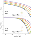 |
Fig. 1. Spectral behavior of the total intensity, for some choices of parameters. Upper panel: Spectra of ℐ, for a fixed choice of s (=2) and β (=1), and different choices of the level of the random MF, here isotropic and characterized by the standard deviation σ. ℐ is normalized by taking |


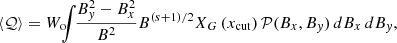
Since the absolute value of the emission strongly depends on quantities (like the particle density and the MF intensity) that are poorly known, in practice the most directly testable quantity is Π. Figures 3 and 4 give, again in the case of an isotropic random MF and the parameters setting described above, the dependence of Π on σ and ν. The bottom side of the plots (low ν/νbr) represent cases still in the power-law region of the spectrum, while their left-hand side represents cases with a very low random field component. The classic value Πo, which is 0.69 for s = 2, is approached near the bottom left corner.
 |
Fig. 3. Iso-level representation of the Π dependence on the level of the (isotropic) random MF and on the frequency, for cases with s = 2, β = 1. The homogeneous case is approached at the left edge of the figure, while at the bottom edge we have a good approximation of the power-law case. |
The conclusion is that Π is generally higher in X-rays than at the lower frequencies (e.g., in the radio band). This trend can be easily understood if we note that first, the absolute value of the local spectral index around the cutoff is higher than in radio and second, Π is higher for larger values of s. The local spectral index, a concept also used in the following, is evaluated on a narrow spectral range by fitting the local spectrum with a power law.
The increase in Π with s may approximately be verified, for the simplified case of a completely ordered MF, by using Eq. (25) with the local s value corresponding to the local spectral index α (defined as dlnI/dlnν), namely s = 1 − 2α. The exact value of the polarization degree is Πo times the ratio of the quantities XG to XF. These two quantities are defined in Eqs. (21) and (22), and their ratio is also displayed in the lower panel of Fig. B.1, still in the case of a homogeneous MF, corresponding to the left edge of Figs. 3 and 4.
For the numerical evaluation of the integrals in Eqs. (23) and (24) we used the approximations described in Appendix B (Eqs. B.9 and B.10, complemented by the coefficients in Tables B.1 and B.2). By comparing them (for all the cases with s = 2 and β = 1), with a direct interpolation of numerically evaluated cases, we find that the estimates of Π obtained with the two methods coincide within a tolerance of 0.05%, for all frequencies smaller than 100 ωcut, while a somewhat worse accuracy appears at frequencies larger than 100 ωcut (a range of much less importance, due to the rapid cutoff in the emission).
2.2. The case of a purely anisotropic random field
Another class of cases, for which in Paper I we have found analytical solutions, consists of those with a negligible ordered MF ( ) and an anisotropic random MF with symmetry axes along x and y (with standard deviations respectively equal to σx and σy). Following Paper I, we define
 (27)
(27)
The defined quantity fan ranges from −1 (σx ≫ σy) to +1 (σy ≫ σx). Alternatively, we may write
 (28)
(28)
In a similar way to the previous section, Figs. 5 and 6 show the total intensity profiles.
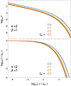 |
Fig. 5. Spectra for ℐ, as plotted in Fig. 1, but for the anisotropic case, with |

The most interesting behavior is for Π, and it is shown in Figs. 7 and 8, for s = 2 and, respectively, β = 1 and β = 2. Also in this case Π increases with frequency around the spectral cutoff.
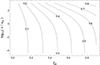 |
Fig. 7. Iso-level representation of the Π dependence on the anisotropy of the random MF and on the frequency, for cases with s = 2, β = 1, and different levels of random MF anisotropy and frequency. Here only the positive values of fan are shown, but the pattern is symmetric with respect to fan = 0. Changing the sign of fan is equivalent to exchanging x and y. The case fan = 0 is equivalent, for the results in the previous section, to the asymptotic case |

3. Observable quantities
In the previous section we show how total emission and polarization change with frequency, there scaled with νbr. We should note however that, in order to derive νbr from observations, measurements should be available over a wide spectral range (for SNRs, typically from the radio to the X-rays); in addition a fitting strategy is required, which means that the result is model-dependent (in our case, it would depend on what value of β is assumed for the fit); the final best-fit values will also depend on which spectral ranges are used; last but not least, typically (at least in SNRs) the region emitting in radio is thicker than that in X-rays, which means that the emission at lower frequencies is overestimated, and as a consequence νbr is underestimated: this problem is rather general, but it is better elucidated in Sect. 4 with reference to the case of SN 1006.
A standard model for these spectra is SRCUT (Reynolds & Keohane 1999), also implemented in the XSPEC package: essentially, it assumes synchrotron emission by a power-law distribution of electrons with an exponential cutoff (β = 1 in our notation).
While it is possible to envisage a generalization of that model to allow different values of β as well as different levels of the random MF component, in this section we discuss some relations that depend only on directly observed quantities: 1. the local spectral index, that measured using only data in a narrow spectral range; 2. the polarization level in the same spectral range; 3. the spectral curvature, a variation with frequency of the local spectral index. Of course, interesting data are obtained only when considering sufficiently high frequencies to measure the effects of the cutoff on the particle distribution. For SNRs, this typically happens in the X-rays spectral range, and so in the following we explicitly refer to it.
3.1. Polarization degree
In Sect. 2.1 we mention an increase in Π close to the spectral cutoff and beyond. Here we discuss in more detail the dependence of Π on the local spectral index. Figure 9 shows its behavior in the case of an isotropic random MF component, for several levels of the random MF magnitude. The cases with β = 1 are shown as dashed curves, while those with β = 2 as solid curves. The two families of curves are almost superimposed, which means that they are very poorly sensitive to the value of β; this then represents a good measurement of the level of the random MF. The same result occurs for the anisotropic case (and  ). As shown in Fig. 10, the two families of curves depend on the value of fan, but very poorly on the value of β, in the considered range. The regions with more extreme local spectral indices are well beyond the cutoff, so that they would be very faint and hard to be detected.
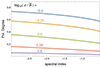 |
Fig. 9. Dependence of Π on the local spectral index α, for s = 2 and various levels of the isotropic random fields. The choice of the levels is the same as in Fig. 1: it starts with |

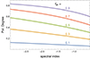 |
Fig. 10. Same as Fig. 9, but for cases of anisotropic random MF, and |

3.2. Spectral curvature
A further observable could be considered, even if more difficult to measure, namely the curvature of the spectrum in the X-ray region, defined here as the derivative of the local spectral index with respect to the logarithm of the frequency dα/dlnν. It requires a wide X-ray spectral range to be measured, while for the main imaging telescopes the width of the X-ray spectral window does not extend beyond ≃10 keV. Only recently have the required conditions been achieved by combining for instance XMM-Newton and NuSTAR data (see, e.g., Li et al. 2018).
Figures 11 and 12 show that the spectral curvature (i.e., how much the shape of the synchrotron spectrum deviates from a pure power law), as a function of the local spectral index, is sensitive to the type of cutoff (i.e., to the parameter β), while it is almost insensitive to the level of the random field component, both in the isotropic and the anisotropic case (with  ). Therefore, the measurement of the spectral curvature could be very effective for investigating the physical nature of the spectral cutoff. The only problem could be in principle that the emitting region could not be exactly the same at all X-ray frequencies: a caveat similar to that about the comparison between radio and X-ray emission, but now much less relevant because the spectral lever is hardly wider than just one decade.
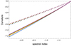 |
Fig. 11. Dependence of the curvature on the local spectral index α, for s = 2 and various levels of the isotropic random fields (same choice of levels as in Fig. 1). The dashed lines refer to cases with β = 1, while the solid lines to β = 2. In this case, the trends are rather insensitive to the level of the random MF, while they are mostly sensitive to the value of β. |
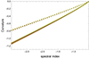 |
Fig. 12. Same as Fig. 11, but for cases of anisotropic random MF (plus |

3.3. Accuracy of the analytic formulae
One could wonder how well a real case with curved spectrum in X-rays can be approximated by the analytic solutions for a purely power-law distribution (Paper I), in the isotropic case and in the anisotropic case (and  ). Figure 13 shows, for our models with an isotropic random MF, the difference between the numerically evaluated Π and the analytic formulae from our Paper I, when applied to the local spectral index, after fitting the local spectrum with a power law. Even if the spectrum is bent, because of its proximity to the cutoff (as is usually the case for SNRs in the X-ray spectral range), the figure proves that our analytic formulae are generally very good approximations of the real cases. The numerically determined values of Π are always larger than the analytic approximations, but with a discrepancy always smaller than 0.01. A similar conclusion can also be obtained for the case of an anisotropic random MF, as shown in Fig. 14.
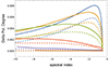 |
Fig. 13. Difference between the numerically evaluated Π and the analytic approximation for a power-law distribution, for all of our models with an isotropic random MF. The difference is always lower than 0.01. |
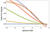 |
Fig. 14. Same as Fig. 13, but for the case of an anisotropic random MF (plus |

4. Application to some young SNRs
The young supernova remnant SN 1006, with its wide angular size and rather ordered morphology, represents an optimal source for a spatially resolved analysis of synchrotron radiation, both in the radio and in the X-rays (also this one dominated by nonthermal emission).
To get a reliable estimate of the cutoff frequency (νbr in our notation), one would need to measure the emission from a fixed volume element, with homogeneous physical conditions. Instead, by a comparative analysis of the radio and X-ray patterns for SN 1006 (see, e.g., Rothenflug et al. 2004; Petruk et al. 2009), one can infer that the X-ray limb is much thinner than that in radio. This difference is likely due to the different synchrotron lifetimes of the emitting electrons, in the downstream, and it is a common characteristics of young SNRs.
This means that (in addition to other possible changes of conditions) the emitting domain along a given LoS is longer at lower frequencies: close to the projected edge of the SNRs the effect of this bias could be marginal, but it is more consistent for a LoS not as close to the SNR edge. The result is to underestimate the X-ray emissivity with respect to the radio value, and consequently to underestimate the cutoff frequency. This effect easily justifies the maps of cutoff frequency presented in some papers, among which Katsuda et al. (2010) and Li et al. (2018), which show a strong radial gradient for this quantity. A similar effect also takes place in the presence of MF inhomogeneities inside the SNR, even though under usual conditions the main effect is expected to derive from the energy dependence of the synchrotron radiative time.
The least biased measurements of νbr are those taken very close to the SNR projected edge; even though a slight wrinkling at the edge would be enough to distort those measurements as well. This case also justifies why, in our previous modeling, we searched for relations between actually observed quantities, and that do not depend on the actual value of νbr, a quantity hard to evaluate in an unbiased and model independent way.
Using the polarization measurements in Zhou et al. (2023) (their Table 1), in Fig. 15 we show that Π in radio and that in the X-rays agree with each other, which could mean that, in spite of the different extensions of the emitting region in these two spectral ranges, the data are consistent with the properties of the random MF component being the same. In the upper panel the data are superimposed to models of a homogeneous MF plus an isotropic random component: the various data are compatible with 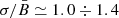 ; we note that in their paper the symbol σB is used instead of our σ. The values of σ for an isotropic random field are upper limits since they are estimated in the limit case that
  keeps constant along the whole LoS. As already mentioned by Zhou et al. (2023), these values are lower than the magnetic amplification expected theoretically, and in some cases derived from the sharp profiles of the nonthermal X-ray filaments.
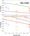 |
Fig. 15. Comparison of the radio and X-ray polarization data on SN 1006 Zhou et al. (2023, data as from). The upper panel shows them superimposed to models of a homogeneous MF composed with an isotropic random component (the labels indicate |

In the lower panel, instead, the data are superimposed to models of an anisotropic random MF, at a level much higher than any ordered background MF: in this case the data are compatible with fan ≃ 0.2 ÷ 0.3, with the width of the probability function larger in the radial direction. In order to have a fan with positive sign, consistently with Eq. (27), we assume in the present section the y direction to be parallel to the shock velocity (from which σy ⇒ σ∥), while the x direction perpendicular to it (from which σx ⇒ σ⊥). In other words, we can measure the ratio σ∥/σ⊥ (> 1) in the downstream by using fan as derived from actual measurements of Π and α.
With the present-day polarization data there is no reason to prefer one model to the other, although we note that in the first case the estimated level of the random MF would not comply with a high MF amplification in the upstream, usually taken as a necessary condition for having a high acceleration efficiency, as in the case for SN 1006. On the other hand, our second model is compatible with the idea that the shock is an efficient cosmic-ray accelerator, and for this reason we think it should be preferred.
A random MF preferentially oriented along the radial direction is more likely understood as the effect of motions, driven by some hydrodynamic instability. A well-known mechanism is the Rayleigh-Taylor instability, which occurs when the density is gradient opposite to the pressure gradient. The role of this instability on the development of radially oriented MFs in SNRs was first discussed in detail by Jun & Norman (1996). On the other hand, the Rayleigh-Taylor instability resulted to be mostly effective only near the contact discontinuity, while radially oriented MFs are observed also in the region ahead of the contact discontinuity, approaching the forward shock. The Richtmyer-Meshkov instability then resulted to be more promising to explain the observed phenomenology. This instability originates from corrugations of the shock surface, related to inhomogeneities in the ambient medium. Its role in generating radially oriented MFs has been investigated by Inoue et al. (2013). A detailed analysis of these two instabilities is beyond the scope of the present work; for more details we refer, for instance, to the review by Zhou et al. (2021).
More generally, a disordered magnetic field could be generated in the upstream and in the downstream. In the case some random field (with dispersions σu, ∥ and σu, ⊥) is already present in the upstream, after the compression at the shock the perpendicular spread would change to κ σu, ⊥, where κ is the shock compression factor. Then, given an observed random MF downstream with dispersions σ∥ and σ⊥, the random MF generated in the downstream should be with
 (29)
(29)
 (30)
(30)
It may be seen that, for a negligible random field in the upstream, the spread ratio σg, ∥/σg, ⊥ for the generated random MF is equal to the measured σ∥/σ⊥. Instead, for an isotropic random field in the upstream, there should be σg, ∥/σg, ⊥ > σ∥/σ⊥. In contrast, without MF generation in the downstream, in order to have a measured σ∥/σ⊥ > 1 in the downstream, a highly anisotropic random field would be required in the pre-shock region, with σu, ∥/σu, ⊥ > κ. The fact that the resulting orientation of this anisotropy is radial in SN 1006, contrary to what expected in the case of a mere shock compression of a pre-existing (isotropic) random MF, then suggests that the mechanism driving a radial orientation of this MF downstream must be very efficient.
In a similar way, one can extract some information from X-ray polarization measurements of Tycho. Ferrazzoli et al. (2023), on the basis of IXPE data, obtained measures of the X-ray polarization degree Π, and the local spectral index α, in some selected regions. Among these values were Π = 11.9 ± 2.2% and α = −1.82 ± 0.02 in the rim region; Π = 23.4 ± 4.2% and α = −1.90 ± 0.04 in the west region (denoted (f) in that paper). Using the formulae from our Paper I, Ferrazzoli et al. (2023) derive, respectively, 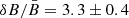 and
and 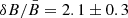 . We note that in that paper the quantity
  is used3, while in our notation those measurements correspond respectively to
  and to
  . We note that also in this case a moderate MF amplification is estimated, contrary to the large amplification theoretically required. On the other hand, a dominant anisotropic random field could reproduce the data, provided that the anisotropy factor is fan = 0.12 ± 0.02 in the first case, and fan = 0.24 ± 0.04 in the second case. According to Eq. (28), these values correspond respectively to σ∥/σ⊥ = 1.13 ± 0.03 and 1.28 ± 0.06. Unfortunately, differently from Zhou et al. (2023), in this paper there are no comparative results on Π in radio for the same regions, so that it is not possible to display for Tycho a figure similar to Fig. 15.
Finally, Vink et al. (2022) reported the results of IXPE observations of Cas A. Unfortunately, given the small angular size of this SNR, it cannot be resolved as well as in the other two cases. In order to optimize the spatial information, the authors have imposed a circular symmetry for the polarization vectors, and have corrected for the thermal X-ray emission. Even so, the X-ray polarization degree is in the range ∼2 − 5%, which is lower than the ∼5% in the radio band, a result apparently impossible, since the spectral index in X-rays is steeper than that in radio. If this result of the data analysis is confirmed, the most reasonable explanation could be that the radio emission comes from a layer substantially thicker than the X-rays, so that the radio and X-ray emitting electrons interact with random fields having either different  or different fan. Apart from this general consideration, however, the quality of these data is not sufficient to perform any accurate model fitting.
5. Homogeneous + anisotropic random field
The result given in Sect. 3.3 is comforting, on the one hand, because is proves that the original analytic formulae (from our Paper I) allow us to reach a good accuracy with a minimum effort; on the other hand, it may appear rather frustrating if all the numerical machinery developed in the present work has served just to test the level of accuracy of our previous analytic functions, when applied to the X-ray polarization, by using the local spectral index. This is not actually the case because the numerical method presented here tackles a much wider variety of problems that could not be investigated analytically.
As an example, we model here the case of a nonnegligible homogeneous MF combined with an anisotropic random MF. In particular, we consider the case of a strong shock, with compression factor κ = 4, moving through an ambient medium characterized upstream by a homogeneous MF component ( ), combined with an isotropic random component (σu). We consider here the case when the only effect of the shock is related to the compression of matter and MF. This should be a rather common case for not too young SNRs.
After the shock passage, in the downstream the field component along the shock velocity remains unchanged, while those orthogonal to it would be enhanced by a factor κ, both for the ordered component ( ,
,  ) and the random one (σd, ∥ = σu, ∥, σd, ⊥ = κ σu, ⊥). The case with a negligible homogeneous component is analyzed in Sect. 2.3 of Paper I. Even in the simplified case of a power-law distribution, with respect to Paper I here we have to add two additional parameters describing the MF conditions upstream: the ratio of random to ordered MF magnitudes (
 ), and the direction of the ordered MF with respect to the direction of the shock velocity (θu), both in the upstream.
Here we restrict our analysis to pure power-law particle energy distributions, but with a similar effort the case with a spectral cutoff one could also be considered. As already shown in Sect. 3.3 for similar cases, results valid for pure power-law distributions could also be accurate enough in the more general case, simply using the local spectral index. Figures 16, 17, and 18 display the results for power-law particle energy distributions with indices s = 2, s = 4, and s = 6, respectively, which correspond to spectral indices α = −0.5, −1.5, and −2.5. Each figure shows the level of Π (upper panel) and the direction of the (magnetic) polarization with respect to the normal to the shock surface.
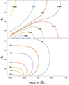 |
Fig. 16. Map of Π (upper panel) and of the (magnetic) polarization direction θs (in degrees, from the direction of the shock velocity), for a wide choice of upstream MF conditions. Here the particle distribution has a power-law index s = 2, corresponding to a spectral index α = −0.5. |
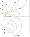 |
Fig. 17. Same as Fig. 16, with a particle power-law index s = 4, corresponding to a spectral index α = −1.5. |
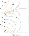 |
Fig. 18. Same as Fig. 16, with a particle power-law index s = 6, corresponding to a spectral index α = −2.5. |
It should be noted that the qualitative trends in these three figures are similar. In particular, the lower panels show very similar behaviors, with differences noticeable only for small values of θd. These trends can be interpreted as follows: in the case of a very low level of the random MF upstream ( ), Π approaches the limit value for a homogeneous MF (Eq. 25), while its direction is always larger than θu, being the MF direction downstream θd = arctan(κ tan(θu)). Instead, in the case
  , the value of θd is always very close to 90°, while Π approaches the analytic values given by Eq. (42) in Paper I. In the intermediate cases we see that, at fixed θu, the value of θd increases monotonically with
  . The value of Π decreases monotonically only for large enough values of θu; for smaller values of θu, instead, the behavior of Π with
  experiences a minimum, essentially when the ordered and the random MF components are of comparable strength, but one is predominantly parallel to the shock velocity, while the other is perpendicular to it, so that their different polarizations tend to eliminate each other.
6. Conclusions
In this paper, which is a continuation of our Paper I, we outlined the basics of our general theory. We described a numerical implementation that allows the spectral behavior of the synchrotron emission and of its polarization degree to be calculated in an efficient way for a wide variety of cases in which an ordered MF component is complemented with a random one.
Our aim was to extend the application of the theory to the X-ray polarization. We first performed an analysis of the two cases already treated in Paper I, namely an isotropic random MF plus an ordered MF, and the anisotropic random MF with a vanishing ordered one, but for a particle energy distribution with an exponential or super-exponential cutoff. While the true cutoff frequency is hard to measure, we discussed the relationships between directly observable quantities, such as the local spectral index (that computed in a limited spectral band), the local spectral curvature, and the polarization degree. We also showed that, with a reasonable level of approximation, our previous analytic formulae computed for a pure power-law case could also be used in a more general case, by applying them to the local spectral index, for example in the presence of a cutoff. We then applied some of our findings to the X-ray polarization results, based on IXPE data, for the young remnants of supernovae SN 1006, Tycho, and Cas A. Finally, we treated the case of a mixture of homogeneous and anisotropic random MF, specialized to the case in which a strong shock compresses an ambient field also with a random component; this case should be of particular interest for the radio emission from mid-age SNRs. As discussed in Sect. 2, the present treatment assumes a large number of MF realizations along a LoS. Moreover, in the presence of MF gradients in the SNR interior as a result of the MHD evolution of plasma, as in Petruk et al. (2017), this condition must also apply for the length scale of such variations. The extension to the X-ray band has made polarimetry an even more important diagnostic tool for studying synchrotron emission from astrophysical sources.
For the frequency we often use the variable ω = 2πν, so that P(ν) = 2π P(ω).
This is the same angle as between the axis x an the E-polarization direction. It is measured in the same direction as the angle of rotation due to the Faraday effect.
The authors consider δB as the dispersion of the module of the random MF vector, in the 3D space, while our σ corresponds to that of its 1D component. In addition, the quantity B in that paper corresponds to our  ; it is the 2D projection of the 3D ordered MF component (we call it Bo). If the value δB/Bo refers to the ratio of the magnitudes of the 3D vectors, then the general way to convert our
  to this ratio is
 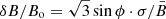 where ϕ is the angle between the LoS and Bo. If we consider a radial ordered MF and regions close to the edge of the SNR projection, then sin ϕ = 1.
Acknowledgments
This work has been partially funded by the European Union – Next Generation EU, through PRIN-MUR 2022TJW4EJ. RB also acknowledges support from the Italian National Institute for Astrophysics with PRIN-INAF 2019 and MiniGrants PWNnumpol and HYPNOTIC87A. OP acknowledges the OAPa grant number D.D.75/2022 funded by Direzione Scientifica of Istituto Nazionale di Astrofisica, Italy. This project has received funding through the MSCA4Ukraine project, which is funded by the European Union. Views and opinions expressed are however those of the authors only and do not necessarily reflect those of the European Union. Neither the European Union nor the MSCA4Ukraine Consortium as a whole nor any individual member institutions of the MSCA4Ukraine Consortium can be held responsible for them. The numerical and analytical calculations presented in this article, as well as the figures shown, were obtained using Wolfram Mathematica.
References
- Bandiera, R., & Petruk, O. 2016, MNRAS, 459, 178 [NASA ADS] [CrossRef] [Google Scholar]
- Bucciantini, N., Ferrazzoli, R., Bachetti, M., et al. 2023, Nat. Astron., 7, 602 [NASA ADS] [CrossRef] [Google Scholar]
- Churazov, E., Khabibullin, I., Barnouin, T., et al. 2024, A&A, 686, A14 [NASA ADS] [CrossRef] [EDP Sciences] [Google Scholar]
- Ferrazzoli, R., Slane, P., Prokhorov, D., et al. 2023, ApJ, 945, 52 [NASA ADS] [CrossRef] [Google Scholar]
- Inoue, T., Shimoda, J., Ohira, Y., & Yamazaki, R. 2013, ApJ, 772, L20 [NASA ADS] [CrossRef] [Google Scholar]
- Jun, B.-I., & Norman, M. L. 1996, ApJ, 472, 245 [Google Scholar]
- Katsuda, S., Petre, R., Mori, K., et al. 2010, ApJ, 723, 383 [NASA ADS] [CrossRef] [Google Scholar]
- Li, J.-T., Ballet, J., Miceli, M., et al. 2018, ApJ, 864, 85 [CrossRef] [Google Scholar]
- Liu, K., Xie, F., Liu, Y.-H., et al. 2023, ApJ, 959, L2 [CrossRef] [Google Scholar]
- Petruk, O., Bocchino, F., Miceli, M., et al. 2009, MNRAS, 399, 157 [NASA ADS] [CrossRef] [Google Scholar]
- Petruk, O., Bandiera, R., Beshley, V., Orlando, S., & Miceli, M. 2017, MNRAS, 470, 1156 [NASA ADS] [CrossRef] [Google Scholar]
- Reynolds, S. P., & Keohane, J. W. 1999, ApJ, 525, 368 [NASA ADS] [CrossRef] [Google Scholar]
- Rothenflug, R., Ballet, J., Dubner, G., et al. 2004, A&A, 425, 121 [NASA ADS] [CrossRef] [EDP Sciences] [Google Scholar]
- Rybicki, G. B., & Lightman, A. P. 1986, Radiative Processes in Astrophysics (Wiley-VCH) [Google Scholar]
- Vink, J., Prokhorov, D., Ferrazzoli, R., et al. 2022, ApJ, 938, 40 [NASA ADS] [CrossRef] [Google Scholar]
- Weisskopf, M. 2022, AAS/High Energy Astrophysics Division, 54, 301.01 [NASA ADS] [Google Scholar]
- Zhou, Y., Williams, R. J. R., Ramaprabhu, P., et al. 2021, Phys. D Nonlinear Phenom., 423, 132838 [NASA ADS] [CrossRef] [Google Scholar]
- Zhou, P., Prokhorov, D., Ferrazzoli, R., et al. 2023, ApJ, 957, 55 [CrossRef] [Google Scholar]
- Zirakashvili, V. N., & Aharonian, F. 2007, A&A, 465, 695 [NASA ADS] [CrossRef] [EDP Sciences] [Google Scholar]
Appendix A: Fits to the F(x) and G(x) functions
In detailed calculations of the synchrotron emission we need to use two special functions, F(x) and G(x) (with x ≥ 0), defined by Eqs. 3 and 4 in the main text. These functions, based on modified Bessel functions of the second kind, and on a related integral, are rather heavy to compute numerically. Since the standard asymptotic approximations
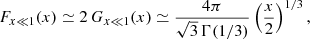 (A.1)
(A.1)
 (A.2)
(A.2)
are limited to respectively very small or very large values of x, we devised fits that, joined together, are valid over the whole range of the argument x and allow a very high accuracy (∼10−6 in the worst case).
For F(x) and x < 1 we applied to the asymptotic approximation the correction factor
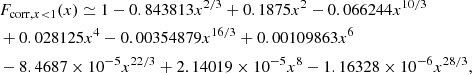 (A.3)
(A.3)
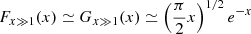
obtained with a more extended power-law expansion. Instead, for x > 1, we started from a slightly more accurate asymptotic solution,
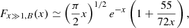 (A.4)
(A.4)
and we then applied a correction of the form 1 − exp(f(lnx)) (where ln is the natural logarithm). By performing a numerical fit we then derived
 (A.5)
(A.5)
In conclusion, an excellent fit to F(x), everywhere better than about 10−6 and usually much better than this, is
![Mathematical equation: $$ \begin{aligned} F(x)=\left\{ \begin{array}{ll} F_{x\ll 1}(x)\cdot F_{\rm {corr,\,} x < 1}(x)&\mathrm{for\,}x < 1 \\ F_{x\gg 1,B}(x)\cdot (1-\exp (f(\ln x))&\mathrm{for\,}x\in [1,720] \\ F_{x\gg 1,B}(x)&\mathrm{for\,}x>720 \end{array}. \right. \end{aligned} $$](/articles/aa/full_html/2024/09/aa50103-24/aa50103-24-eq80.gif) (A.6)
(A.6)
In a similar way, for G(x), we found the x < 1 correction
 (A.7)
(A.7)
the more accurate asymptotic solution
 (A.8)
(A.8)
and the correction for x > 1 based on the fitted function
 (A.9)
(A.9)
so that G(x) can be approximated, again to better than about 10−6, by using
![Mathematical equation: $$ \begin{aligned} G(x)=\left\{ \begin{array}{ll} G_{x\ll 1}(x)\,G_{\rm {corr,\,} x < 1}(x)&\mathrm{for\,}x < 1 \\ G_{x\gg 1,B}(x),(1-\exp (g(\ln x))&\mathrm{for\,}x\in [1,720] \\ G_{x\gg 1,B}(x)&\mathrm{for\,}x>720 \end{array}. \right. \end{aligned} $$](/articles/aa/full_html/2024/09/aa50103-24/aa50103-24-eq84.gif) (A.10)
(A.10)
Appendix B: Fits to some integrals
Let us introduce the quantities
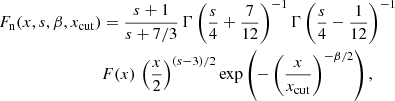 (B.1)
(B.1)
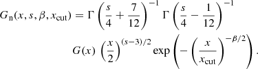 (B.2)
(B.2)
They are normalized in such a way that
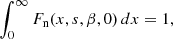 (B.3)
(B.3)
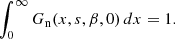 (B.4)
(B.4)
The parameters xcut and β correspond to those introduced in the main text, when we started considering a particle distribution with an energy cutoff (see Eq. 10). We note that xcut = 0 corresponds to γcut = ∞, namely to the case of a power-law distribution, the case already treated in Paper I.
Aim of this Appendix is to evaluate the integral quantities
 (B.5)
(B.5)
 (B.6)
(B.6)
which are fundamental for the aims of the present work.
To rephrase in an explicit form what is already present in Eqs. 5, 15, 16, and 17, the Stokes parameters in the case of a homogeneous MF and a particle energy distribution (Eq. 10) can be expressed as
 (B.7)
(B.7)
 (B.8)
(B.8)
Unfortunately, the integrals in Eqs. B.5 and B.6 do not seem to admit exact analytical solutions, so we computed them numerically in some specific cases, and then devised analytic approximations to them.
As shown in Fig. B.1, the XF curves (upper panel) decrease very rapidly, at large xcut values; this behavior is more prominent for larger values of β. The behavior of XG is similar, so that their ratio (lower panel) is confined, between 1 and (s + 7/3)/(s + 1), and the transition region is narrower for larger values of β. Asymptotically for xcut → ∞, both XF and XG seem to vanish very rapidly.
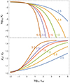 |
Fig. B.1. Plots of log10XF and of XG/XF, for the case s = 2 and several values of β, equal to 0.5, 0.8, 1.0, 15, 2.0, 5.0. |
To fit their behavior over the whole range of xcut, we chose the following approximating formulae:
 (B.9)
(B.9)
 (B.10)
By construction both formulae approach 1 for xcut → 1, while  approaches (s + 7/3)/(s + 1) for large values of xcut.
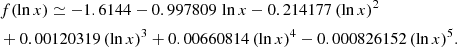
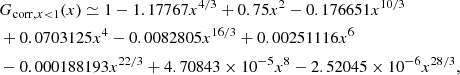
Tables B.1 and B.2 list the best-fit coefficients for a number of choices of s and β. The number of digits chosen for each coefficient is the minimum required to avoid the accuracy of the approximation to be appreciably downgraded by this truncation: in particular, the coefficients b and d require a seven-digit accuracy. The range of the xcut values for the numerical arrays, on which to perform the fits, was chosen to be very wide, from 3 × 10⁻⁷ to 3 × 10⁶, with the exception of higher values of β, when the machine numerical underflow limits the extension of the upper boundary (by a factor ∼5 for β = 1.5, or ∼30 for β = 2.0). In order to give an idea of the level of the accuracy reached, the last column of each table gives the maximum deviation of the approximation. The values in this column are even too conservative; for instance, in Table B.1 typically the largest deviation occurs close to the upper limit of xcut, where the value of XF is extremely low, and inessential for the calculation of other quantities.
Best-fit coefficients (a, b, c, d, e), to adopt for the function  , in order to approximate the function XF(s, β, xcut), for various choices of the parameters s and β. The last column gives the maximum deviation, in absolute value, of the approximation.
Same as Table B.1, but for XG(s, β, xcut)/XF(s, β, xcut). The best-fit coefficients are (f, g, h).
An interesting dependence is how the asymptotic exponential power (d) for XF (and for XG as well), at large values of xcut, changes with β; this dependence is shown in Fig. B.2. First of all, it is clear that it is not a linear dependence. For very low values of β, the value of d is well approximated by β/2, but then it soon flattens, so that for β = 5 the value of d only reaches 0.7177. Due to numerical underflows at large values of β and xcut (see above), its trend at larger values of β is not sufficiently reliable to verify whether it saturates at a maximum value, and no analytical solutions have been found so far, even in these limiting cases.
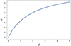 |
Fig. B.2. Dependence of the asymptotic exponential power (d) in XF, as a function of β. |
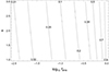 |
Fig. B.3. Map of Π/Πo for anisotropic fluctuations and a vanishing ordered MF (the correct version of Fig. 4 in Paper I). |
Appendix C: Errata corrige to Paper I
We take the opportunity in this Appendix to correct two errors present in Paper I.
First, a misprint in the second line of Eq. 21: instead of  , the formula should have been written
  . However, we point out that the final formula, in the third line of that equation, is correct.
Second, in Fig. 4: In spite of the labels on the axes, for this figure we had erroneously used the same data matrix as for the isotropic case. The correct version is now shown in Fig. B.3. We note that now, as also intuitively expected, the polarization degree increases with increasing anisotropy parameter fan.
All Tables
Best-fit coefficients (a, b, c, d, e), to adopt for the function , in order to approximate the function XF(s, β, xcut), for various choices of the parameters s and β. The last column gives the maximum deviation, in absolute value, of the approximation.
Same as Table B.1, but for XG(s, β, xcut)/XF(s, β, xcut). The best-fit coefficients are (f, g, h).
All Figures
|
Fig. 1. Spectral behavior of the total intensity, for some choices of parameters. Upper panel: Spectra of ℐ, for a fixed choice of s (=2) and β (=1), and different choices of the level of the random MF, here isotropic and characterized by the standard deviation σ. ℐ is normalized by taking |
| In the text | |
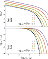 |
Fig. 2. Same as Fig. 1, but for β = 2. |
| In the text | |
|
Fig. 3. Iso-level representation of the Π dependence on the level of the (isotropic) random MF and on the frequency, for cases with s = 2, β = 1. The homogeneous case is approached at the left edge of the figure, while at the bottom edge we have a good approximation of the power-law case. |
| In the text | |
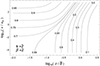 |
Fig. 4. Same as Fig. 3, but for cases with β = 2. |
| In the text | |
|
Fig. 5. Spectra for ℐ, as plotted in Fig. 1, but for the anisotropic case, with |
| In the text | |
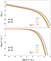 |
Fig. 6. Same as Fig. 5, but with β = 2. |
| In the text | |
|
Fig. 7. Iso-level representation of the Π dependence on the anisotropy of the random MF and on the frequency, for cases with s = 2, β = 1, and different levels of random MF anisotropy and frequency. Here only the positive values of fan are shown, but the pattern is symmetric with respect to fan = 0. Changing the sign of fan is equivalent to exchanging x and y. The case fan = 0 is equivalent, for the results in the previous section, to the asymptotic case |
| In the text | |
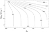 |
Fig. 8. Same as Fig. 7, but for β = 2. |
| In the text | |
|
Fig. 9. Dependence of Π on the local spectral index α, for s = 2 and various levels of the isotropic random fields. The choice of the levels is the same as in Fig. 1: it starts with |
| In the text | |
|
Fig. 10. Same as Fig. 9, but for cases of anisotropic random MF, and |
| In the text | |
|
Fig. 11. Dependence of the curvature on the local spectral index α, for s = 2 and various levels of the isotropic random fields (same choice of levels as in Fig. 1). The dashed lines refer to cases with β = 1, while the solid lines to β = 2. In this case, the trends are rather insensitive to the level of the random MF, while they are mostly sensitive to the value of β. |
| In the text | |
|
Fig. 12. Same as Fig. 11, but for cases of anisotropic random MF (plus |
| In the text | |
|
Fig. 13. Difference between the numerically evaluated Π and the analytic approximation for a power-law distribution, for all of our models with an isotropic random MF. The difference is always lower than 0.01. |
| In the text | |
|
Fig. 14. Same as Fig. 13, but for the case of an anisotropic random MF (plus |
| In the text | |
|
Fig. 15. Comparison of the radio and X-ray polarization data on SN 1006 Zhou et al. (2023, data as from). The upper panel shows them superimposed to models of a homogeneous MF composed with an isotropic random component (the labels indicate |
| In the text | |
|
Fig. 16. Map of Π (upper panel) and of the (magnetic) polarization direction θs (in degrees, from the direction of the shock velocity), for a wide choice of upstream MF conditions. Here the particle distribution has a power-law index s = 2, corresponding to a spectral index α = −0.5. |
| In the text | |
|
Fig. 17. Same as Fig. 16, with a particle power-law index s = 4, corresponding to a spectral index α = −1.5. |
| In the text | |
|
Fig. 18. Same as Fig. 16, with a particle power-law index s = 6, corresponding to a spectral index α = −2.5. |
| In the text | |
|
Fig. B.1. Plots of log10XF and of XG/XF, for the case s = 2 and several values of β, equal to 0.5, 0.8, 1.0, 15, 2.0, 5.0. |
| In the text | |
|
Fig. B.2. Dependence of the asymptotic exponential power (d) in XF, as a function of β. |
| In the text | |
|
Fig. B.3. Map of Π/Πo for anisotropic fluctuations and a vanishing ordered MF (the correct version of Fig. 4 in Paper I). |
| In the text | |
Current usage metrics show cumulative count of Article Views (full-text article views including HTML views, PDF and ePub downloads, according to the available data) and Abstracts Views on Vision4Press platform.
Data correspond to usage on the plateform after 2015. The current usage metrics is available 48-96 hours after online publication and is updated daily on week days.
Initial download of the metrics may take a while.