| Issue |
A&A
Volume 689, September 2024
|
|
|---|---|---|
| Article Number | A176 | |
| Number of page(s) | 10 | |
| Section | Stellar structure and evolution | |
| DOI | https://doi.org/10.1051/0004-6361/202450034 | |
| Published online | 12 September 2024 | |
Investigating the nature of the 2.4 h-period eclipsing cataclysmic variable W2 in 47 Tuc
1
IRAP, CNRS, Université de Toulouse, CNES, 9 Avenue du Colonel Roche, 31028 Toulouse, France
2
INAF-Osservatorio Astronomico di Roma, Via Frascati 33, 00078 Monteporzio Catone, Italy
3
INAF-Istituto di Astrofisica Spaziale e Fisica Cosmica di Milano, Via A. Corti 12, 20133 Milano, Italy
4
Dipartimento di Fisica, Università degli Studi di Roma “Tor Vergata”, Via della Ricerca Scientifica 1, I-00133 Rome, Italy
5
Scuola Universitaria Superiore IUSS Pavia, Palazzo del Broletto, Piazza della Vittoria 15, 27100 Pavia, Italy
6
INAF-Osservatorio Astronomico di Capodimonte, Salita Moiariello 16, I-80131 Napoli, Italy
7
Dipartimento di fisica e chimica – Emilio Segrè, Università degli Studi di Palermo, Via Archirafi 36, 90123 Palermo, Italy
Received:
19
March
2024
Accepted:
4
July
2024
Abstract
Context. W2 (CXOGlb J002415.8–720436) is a cataclysmic variable (CV) in the Galactic globular cluster 47 Tucanae. Its modulation was discovered within the CATS@BAR project. The source shows all the properties of magnetic CVs, but whether it is a polar or an intermediate polar is still a matter of debate.
Aims. This paper investigates the spectral and temporal properties of the source, using all archival X-ray data from Chandra and eROSITA Early Data Release, to establish whether the source falls within the category of polars or intermediate polars.
Methods. We fitted Chandra archival spectra with three different models: a power law, a bremsstrahlung and an optically thin thermal plasma. We also explored the temporal properties of the source with searches for pulsations with a power spectral density analysis and a Rayleigh test (Zn2).
Results. W2 displays a mean luminosity of ∼1032 erg s−1 over a 20-year span, despite lower values in a few epochs. The source is not detected in the latest observation, taken with Chandra in 2022, and we infer an X-ray luminosity ≤7 × 1031 erg s−1. The source spectral shape does not change over time and can be equally well fitted with each of the three models, with a best-fit photon index of 1.6 for the power law and best-fit temperatures of 10 keV for both the bremsstrahlung and the thermal plasma models. We confirm the previously detected period of 8649 s, ascribed to the binary orbital period, and found a cycle-to-cycle variability associated with this periodicity. No other significant pulsation is detected.
Conclusions. Considering the source orbital period, luminosity, spectral characteristics, long-term evolution and strong cycle-to-cycle variability, we suggest that W2 is a magnetic CV of the polar type.
Key words: novae / cataclysmic variables / globular clusters: individual: 47 Tucanae / X-rays: individuals: W2
Corresponding author; This email address is being protected from spambots. You need JavaScript enabled to view it. .
© The Authors 2024
 Open Access article, published by EDP Sciences, under the terms of the Creative Commons Attribution License (https://creativecommons.org/licenses/by/4.0), which permits unrestricted use, distribution, and reproduction in any medium, provided the original work is properly cited.
This article is published in open access under the Subscribe to Open model. This email address is being protected from spambots. You need JavaScript enabled to view it. to support open access publication.
1. Introduction
Globular clusters (GCs) are the oldest stellar structures in the Milky Way, usually showing nearly spherical distributions, with tens of thousands of stars bound by gravity. Owing to their dense environments, GCs are good laboratories for stellar dynamics and host abundant populations of compact objects, often segregated in their core and formed dynamically (e.g. Pooley et al. 2003). Examples include low-mass X-ray binaries (LMXBs), cataclysmic variables (CVs), recycled millisecond pulsars, and – perhaps – even intermediate mass black holes (Meylan & Heggie 1997; Strader et al. 2012; Lugaro et al. 2013). As the remnants of the least massive stars, which are the most abundant types of stars, white dwarfs (WDs) should be the most common compact objects in GCs. The identification of isolated WDs in GCs is a challenging endeavour due to their intrinsic faintness. On the other hand, the observation of accreting WDs in the UV and X-rays, their characteristics and population ratio with respect to other X-ray emitters are important diagnostics of the cluster evolution and tests of stellar dynamics.
47 Tucanae (NGC 104, 47 Tuc for brevity) is one of the brightest and most massive GC in the Milky Way1. It has a mass of ≃7 × 10⁵ M⊙ (Marks & Kroupa 2010), an age of 12−13 Gyr (Zoccali et al. 2001; García-Berro et al. 2014; Thompson et al. 2020), and various distance estimates: 4.521 ± 0.031 kpc (Baumgardt & Vasiliev 2021), 4.45 ± 0.01 ± 0.12 kpc (Chen et al. 2018), and 4.47 ± 0.01 ± 0.08 kpc (Simunovic et al. 2023); for this work we shall simply assume 4.5 kpc. Several hundreds of CVs are expected to be present in 47 Tuc, as results of both the evolution of primordial binaries and dynamical encounters/three-body interactions (Pooley & Hut 2006; Belloni & Rivera 2021). Data taken with the Chandra X-ray Observatory (Weisskopf et al. 2000) of the core of 47 Tuc showed the presence of more than one hundred faint X-ray sources within a few arcmin (Edmonds et al. 2003a; Heinke et al. 2005). About one-third were tentatively identified with CVs and many were confirmed with subsequent optical/ultraviolet observations (see e.g. Edmonds et al. 2003b; Bhattacharya et al. 2017; Rivera Sandoval et al. 2018). Recently, 47 Tuc has also been observed during the calibration phase of the extended Roentgen Survey with an Imaging Telescope Array (eROSITA, Predehl et al. 2021), where about 888 point-like sources were detected, with a handful identified as CVs (Saeedi et al. 2022).
CXOGlb J002415.8–720436 (W2 hereafter) was first identified as a possible CV candidate (or an enshrouded millisecond pulsar) by Grindlay et al. (2001), who compared Chandra and ROSAT (Truemper 1982) data of 47 Tuc. Edmonds et al. (2003a,b) studied the optical counterparts of all X-ray sources of 47 Tuc with the Hubble Space Telescope (HST) and found for W2 a V magnitude of 21.50 and U − V and V − I colours of 0.04 mag and 1.91 mag, respectively. The location of this source in the U, U − V colour-magnitude diagram was blueward of the main sequence, but close to the main sequence in the V, V − I colour-magnitude diagram. They concluded that the source might have had a relatively faint accretion disc, with the optical magnitude dominated by the companion star. They also suggested that the system had a low accretion rate and estimated an X-ray period of ∼6.3 h, different from the optical periods of 2.2 h, 5.9 h, and 8.2 h (Edmonds et al. 2003a). The spectral analysis of the source was carried out by Heinke et al. (2005) on 2000 and 2002 Chandra data, resulting in X-ray luminosities in the energy range 0.5−6 keV of ∼8 × 1031 erg s−1 and ∼16 × 1031 erg s−1, for the two epochs, respectively.
Israel et al. (2016) unambiguously classified W2 as a CV based on the timing analysis of Chandra ObsIDs. 953, 955, and 2735−8, that revealed an eclipse with a period of 8649 s (2.4 h), ascribed to the binary orbit. Their analysis did not confirm the X-ray period of ∼6.3 h derived by Edmonds et al. (2003a). Rivera Sandoval et al. (2018) further studied the HST data of 47 Tuc in the near ultra-violet (NUV) and optical wavebands. Using the ultraviolet filter U300, they did not find any periodicity of the source for any of the periods previously proposed in the literature. However, the authors selected only high-quality photometric data resulting in a sparse sampling over 8 h of observation, which could well have missed the 8 min long eclipse. Notwithstanding, the light curve showed a variation of 3 mag during the time of the observation. On the other hand, the period of 2.4 h was confirmed in the more intensive coverage with the R625 filter, with the appearance of a deep eclipse-like feature, hence confirming the optical counterpart to W2. The source was classified as a candidate magnetic CV, very likely an intermediate polar (IP), where the variations in magnitudes were attributed to either precession of the accretion disc, or changes of its thickness, or high/low state transitions. The most recent search for periodicity from the source was performed by Bao et al. (2023), who found a first period of 8646.78 s, close to the one of Israel et al. (2016) and ascribed it to the orbital period, and a second one of 3846.15 s, interpreted as the spin period of the WD, supporting the IP scenario. Unfortunately, due to the source density in the central region of 47 Tuc (within a radius of 1.7′), W2 is not resolved by eROSITA (Saeedi et al. 2022).
In this paper, we aim to resolve the controversy on the presence and the nature of the X-ray periods of W2 and classify the source through simultaneous use of X-ray spectroscopic and timing analysis techniques. We use all available Chandra data, including two new observations taken in 2022 (see Table A.1). We also revisit eROSITA Early Data Release (EDR) and detect the source for first time using this dataset, thanks to its period, even if it cannot be spatially resolved from nearby sources. Data reduction, spectroscopic and timing analyses are described in Sects. 2, 3 and 4, respectively. The nature of the source is discussed in Sect. 5 and our conclusions are presented in Sect. 6.
2. Data reduction
2.1. Chandra
All available observations of the Galactic GC 47 Tuc in the Chandra Data Archive span roughly 15 years, from early 2000 to 2015, with the addition of two recent observations, taken in January 2022. For this work we considered all the observations taken with ACIS-S or ACIS-I, as reported in Table A.1. A Chandra image of 47 Tuc is shown in Fig. 1, left panel.
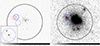 |
Fig. 1. Chandra (left panel, ObsID. 2735) and eROSITA (right panel, 1−2 Nov. 2019 observations) images of the field of view of 47 Tuc. Solid and dashed circles represent the source and background extraction regions for W2, respectively, for Chandra (red) and eROSITA (blue). The black circle encloses the inner region of the cluster excluded in the eROSITA analysis of Bao et al. (2023) and has a radius of 1.7′. The box in the bottom left corner is a close-up of the eROSITA source region as seen by Chandra, to show the X-ray sources that are blended with W2 in the eROSITA image. |
All the data sets were reprocessed with the tool chandra_repro in the Chandra Interactive Analysis of Observations software (CIAO, version 4.14), using calibration files CALDB 4.9.8. The target was identified by means of its sky coordinates, RA =  and Dec =
  , in J2000 reference frame, as in Israel et al. (2016). Spectra and light curves were extracted using the CIAO tool specextract. We used circular regions for both the source and the background, the former (1.8″) centred on the source position, the latter (10″) on a nearby region, which contained no other X-ray sources, on the same CCD. For each observation, we generated the source and background spectra, the redistribution matrix and the auxiliary response files (rmf and arf). Each spectrum was binned with a minimum number of 20 cts/bin. We used the same regions to extract the light curves, after having barycentred the observations at the source coordinates, with the JPL solar system ephemeris DE200. Amongst all the observations, two data sets (954 and 16528) were rejected, because the target was not on the illuminated CCDs.
The source was not visible by eye in the latest observation ObsID. 26286. We ran the CIAO tool wavdetect to see if the algorithm could detect it. We first created exposure-corrected images and exposure maps of the observation using fluximage, in the broad energy band (0.5−7 keV), where the source flux peaks (e.g. Heinke et al. 2005), with the option psfecf = 0.99. We then ran wavdetect, choosing the scales of 1 and 2 to enhance the detection of point-like sources. Seeing as no source was detected at the position of W2, we used the tool aplimits to obtain an upper limit on the count rate. For a false detection probability of 0.1 (corresponding to 90% confidence level, c.l.), a probability of missed detection of 0.5, and a background rate of 7.5 × 10⁻³ cts s−1, estimated from the circular background region of all other observations, we obtained an upper limit of 1.2 × 10⁻³ cts s−1.
2.2. eROSITA
eROSITA observed 47 Tuc during the calibration phase on November 1−2, 2019 (ObsIDs. 700011, 700163, 700013, 700014) and November 19, 2019 (ObsIDs. 700173-175), for a total of ∼101 ks and ∼25 ks, respectively. Another observation was carried out on September 28, 2019 (ObsID. 700012), but we excluded it since no information about the satellite orbit2 is available before October 2019 and no barycentric correction could be applied to the data.
To extract eROSITA data from the EDR observations, we used the eROSITA Standard Analysis Software System (eSASS, see Brunner et al. 2022) available on the EDR webpage3. Following the online guide to eSASS4, we selected all the events in the 0.2−5 keV band with valid patterns (PATTERN = 15) within the nominal field of view (FLAG = 0xc0008000). In Fig. 1 (right panel) we show a close-up view of the eROSITA field during the November 1−2 observations. The solid blue circle denotes the 15″-radius region we used to extract the source events. Note that eROSITA is not able to resolve W2 from the other X-ray sources within the extraction area, which are instead resolved by Chandra (see box in the bottom left corner of Fig. 1). In particular, another CV (W1, see e.g. Heinke et al. 2005), with luminosity comparable to W2, falls within the eROSITA extraction region. This second CV was detected in the 2000 and 2002 Chandra data sets by Heinke et al. (2005), while a visual inspection of the 2014 and 2022 data sets revealed it to be switched off. We have no means to say whether W1 is also present in the eROSITA observations.
3. Spectroscopic analysis
Spectral analysis was performed with the X-Ray Spectral Fitting Package Xspec (Arnaud 1996), version 12.9.1, using abundances from Wilms et al. (2000) and cross-sections from Verner et al. (1996). At first, we considered only the seven observations (ObsIDs. 955, 2735, 2736, 2737, 2738, 15747, 16527), where the source spectrum has at least five data points in the range 0.5−6 keV, suitable for a fit with χ2 statistics. Above 6 keV the spectrum is dominated by the background. Following the analysis by Heinke et al. (2005), we fit them separately with three different emission models: a power law (PL), a thermal Bremsstrahulung (TB), and a vmekal (Mewe 1991) model. Statistical errors are at 90% c.l., unless specified otherwise.
We considered two different components for the interstellar absorption. The first component ( , modelled with TBabs) accounts for the total Galactic absorption in the direction of 47 Tuc and was fixed to 5.5 × 1020 cm−2, according to the estimate provided by the HEASARC NH calculator tool5, assuming Solar abundances. The second component (
 , described by the TBvarabs function) represents both the interstellar absorption within the cluster and local to the source. In this case, we fixed the chemical abundances to those derived from Thygesen et al. (2014) for 47 Tuc, namely 33% of solar abundances for C, N, O, and Ne, 27% for Na and Al, 46% for Mg, 35% for Si, S, and Ar, 34% for Ca, 17% for Fe, and 13% for Ni.
For all three models, the local absorption  was consistent in all the spectra, with the exception of ObsIDs. 15747 and 16527, where it was unconstrained. Hence, we tied the
  values and fitted the seven observations again. The fit converged to
  cm−2. Detailed tables with the best-fit results for both fits and for each model are reported in Appendix B.
The best-fit power law photon index and the temperatures of the TB and vmekal models were consistent for all observations, so that we also tied them together to get more stringent constraints. We obtained a best-fit photon index  and best-fit temperatures of
  keV for both thermal models. According to the fit statistics, all models provide an equally good description of the spectra.
As a side note, for the vmekal model, we considered the same abundances we used for the local absorption component (Thygesen et al. 2014). The total spectrum was then computed by interpolating on a pre-calculated table (parameter switch = 1). Setting the chemical abundances to those of Heinke et al. (2005), leads to little or no difference in the best-fit values. We also note that there is little to no difference in the fit residuals between the two thermal models (Fig. 2), confirming that the two models are equivalent with respect to the quality of the present data sets. We do not include eROSITA data in the spectral analysis, because it is not possible to extract a clean source spectrum, not contaminated by the nearby bright X-ray source W1 (cf. Sect. 2.2 and Fig. 1). This will not be a problem for the timing analysis (Sect. 4).
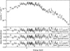 |
Fig. 2. Summed spectra from all the Chandra data sets in which the source was detected, together with the best-fit power-law model (top panel), and residuals in units of |

The consistency of the best-fit parameters of the previous fits demonstrates that W2 does not change its spectral state over time, in spite of changes in flux (the normalisation is changing). Therefore, we decided to combine the spectra of all observations in which the source was detected (Table A.1), to further constrain the best-fit parameters. To combine the spectra, we used the CIAO tool combine_spectra, which sums the counts of each corresponding spectral bin of different spectra and returns a total spectrum. In this way, we increased the number of counts in each spectral bin and achieved a better signal-to-noise ratio (S/N). The combined spectrum was again grouped with 20 cts/bin and fitted with the same models as above. Results of the fits are shown in Table 1 and in Fig. 2, with fluxes and luminosities in the 0.3−10 keV energy range. The fits returned a  (d.o.f.) of 0.94(97) for the PL and of 0.90(97) for both the TB and the vmekal models, with null hypothesis probability (n.h.p.) values of 0.64, 0.75, and 0.74, respectively. The best-fit values of the parameters
  , Γ and kT were all consistent with those obtained in the previous fits. In all cases, the unabsorbed flux is (6–7) × 10−14 erg cm−2 s−1, which results in X-ray luminosities in the range LX = (1.5 − 1.7)×1032 erg s−1, for a distance d = 4.5 kpc.
Best-fit values of the spectrum obtained by combining all the data sets.
Once the best-fit parameters were constrained, we explored the long-term variability of the source, studying the changes in flux over time. To do so, we used the TB model and derived the fluxes for those observations excluded from the previous analysis. We imposed  cm−2 and kT = 10 keV (see Table 1) and fitted the data, leaving only the normalisation free to vary. For the latest Chandra observation, for which we do not have a spectrum, we derived upper limits on the flux and luminosity from the upper limit on the count rate estimated in Sect. 2.1. We used the online tool WebPIMMS6 with the best-fit parameters of the TB model and obtained an X-ray luminosity ≤7 × 1031 erg s−1, in the energy range 0.3–10 keV, at 90% c.l. All resulting fluxes and luminosities are shown in Table 2 and in Fig. 3. In most observations, the source flux is in the range Fabs ∼ (4 − 9)×10−14 erg cm−2 s−1, corresponding to a luminosity LX ∼ (1 − 2)×1032 erg s−1, while in a few it is significantly lower. Some observations (marked with an asterisk in Table 2) are shorter than the orbital period and their luminosities might be unreliable.
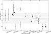 |
Fig. 3. Light curve of W2. Empty data points are for those observations with exposures shorter than the orbital period; the black arrow represents the upper limit at 90% c.l. on the luminosity of the latest Chandra observation (ObsID. 26286); the grey dotted line and area represents the average luminosity of the source and its uncertainty at 90 % c.l., respectively. |
W2 unabsorbed fluxes and luminosities (0.3–10 keV) for each observation.
4. Timing analysis
Israel et al. (2016) found a phase-coherent solution for W2 in ObsIDs. 2735–8 corresponding to a period of 8649 ± 1 s. The eclipse profile was asymmetric and showed a total eclipse lasting about 8 min. The modulation was also present in ObsIDs. 953 and 955, though the poor statistics did not allow an independent period value to be inferred. Among the new available archival observations we focused on ObsID. 15747–8, 16527 and 16529 where the source is detected and the relatively long exposures ensure good statistics. A phase-fitting procedure was applied revealing a period of 8653 ± 3 s, in agreement with that in the CATS@BAR catalogue although with a larger uncertainty. Consequently, we keep the period reported in the catalogue as the reference one in the subsequent analysis.
Recently, Bao et al. (2023) reported a second coherent signal, detected by a Gregory–Loredo algorithm (Gregory & Loredo 1992), corresponding to a period P = 3846.15 s. Our PDS analysis of Chandra observations 2735–8, performed following Israel & Stella (1996), shows no significant peak above the 3.5σ threshold at the corresponding frequency (see Fig. 4, left panel), although the high PDS peak at the frequency of the second harmonic of the 2.4 h modulation, at about 4325 s, hampers the detection sensitivity around the peak itself. To further check for the presence of the reported modulation at ∼3846 s, we also performed a  search (Buccheri et al. 1983) for periodicity in the 0.1−0.6 mHz range, using the henzsearch tool included in the HENDRICS package (Bachetti 2018). The right panel of Fig. 4 shows the results of our analysis. Both the fundamental (ν ≃ 116 μHz, n = 4) and the second harmonic (ν ≃ 231 μHz, n = 1) are clearly detected, while the P = 3846.15 s is below the 3.5σ detection threshold.
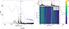 |
Fig. 4. Results of the pulsation searches in Chandra data of W2. Left panel: power density spectrum (PDS) in the 0.2−10 keV energy range by using the 2002 datasets 2735–8 and one single interval. The 3.5σ detection threshold is also shown and marked by the blue solid line. The PDS is complex and only one peak is above the threshold, corresponding to the harmonic of the 8649 s period (both the fundamental and the harmonic are marked by I17 and 1/2P I17, respectively). The period suggested by Bao et al. (2023) is indicated as B23. Right: |

In order to further check the possibility that the peak at P = 3846.15 s might be a spin period we carried out a phase-fitting analysis by using time intervals of 2.4 h length (i.e. over one orbital cycle). If the P = 3846.15 s is real, we expect to see either a constant or a linear trend in the phases. In Fig. 5 we show the results of this analysis ( of 40 for a linear component model) where it is evident that the phases are highly scattered up to almost 40% of the period, suggesting that the peak is spurious and/or marks a variability with a low coherence level such as a QPO-like component. Regardless of the exact origin of the 3846.15 s peak, we can reasonably exclude that it is a strictly coherent signal and, therefore, that it is the spin period of the accreting WD.
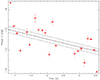 |
Fig. 5. Phase-fitting of the 3846.15 s period of Bao et al. (2023), where each data point corresponds to a duration of one orbital cycle (i.e. 8649 s). The phases are highly scattered up to almost 40% of the period, suggesting that this period is spurious and/or not coherent. The black solid and stepped lines mark the best fit linear component and its 1σ uncertainty, respectively. |
Fig. 6 shows the eclipse profile evolution as a function of time, for P = 8649 s, for the three different epochs (2000, 2002, and 2014, left panel), while the bottom panel shows the eclipse profiles for the 2002 ObsIDs. 2735–8. Note that the sparseness of the observations does not allow for a phase alignment of the three epochs. Hence, we shifted the profiles arbitrarily in order to have the centre of the eclipse aligned at the same phase. In Fig. 7 we show the eclipse profiles of the summed 2002 spectra at different energy ranges (0.3−2 keV, 2−6 keV, and 6−10 keV) and the hardness ratio (2−6 keV/0.3−2 keV). The profiles clearly display a double hump, more evident at soft than hard energies, with the relative intensity of the humps changing both from epoch to epoch and within the same epoch, often on time scales less than a day. The hardness ratio is constant within the uncertainties, except for the eclipse phase, where the counts in all bands are consistent with zero.
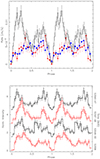 |
Fig. 6. Chandra ACIS eclipse profiles of W2, folded to the best period of P = 8649 s. Top panel: profiles for the three different epochs where the modulation was detected: 2000 (red line and filled circles), 2002 (black lines), and 2014 (blue line and filled squares). A correction of about 20% was applied to the 2000 datasets in order to take into account the difference in CCD efficiency between ACIS-I and ACIS-S. We used the reference epoch MJD 52551.999(1) (1σ c.l.) for the 2002 datasets, while the 2000 and 2014 light curves have been arbitrarily shifted along the x-axis in order to align the minima, corresponding to the 8-min eclipse. All light curves have 20 phase-bins of ∼432 s duration each. Bottom panel: folded light curves of the four longest observations, carried out in 2002 a few days apart from each other. From top to bottom: ObsID. 2735, 2736, 2737 and 2738. The profiles are complex and variable on time scales of less than a day. |
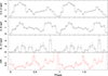 |
Fig. 7. Energy-resolved profiles of the summed 2002 data sets, in units of normalised intensity, for the following energy ranges: 0.3–2 keV (first panel), 2–6 keV (second panel), 6–10 keV (third panel). Bottom panel: hardness ratio (2–6 keV)/(0.3–2 keV). |
To complete our analysis, we searched for the same periodicity of P = 8649 s in the eROSITA data. Both the PDS and  search did not reveal any signal with a significance ≥3.5σ, but epoch folding at the period found in Chandra data returned the same eclipse profile at P = 8649 s. Fig. 8 shows the phase-folded profiles of both eROSITA epochs, where the background has been inferred by also correcting for the expected count rate of the other bright source W1 within the source extraction region (see box in Fig. 1) in the eROSITA energy band, based on the analysis of Heinke et al. (2005) of Chandra archival observations where W1 is detected. W2’s eclipse profile shape is consistent with the one found in the Chandra data (cf. Fig. 6), ultimately proving the detection of the source. We also tried to fold eROSITA light curves at the period of P ≃ 3846.15 s and obtained a profile similar to the one reported by Bao et al. (2023). However, we also found that similar profiles are obtained with any period within the 3746–3946 s range, and indeed at these frequencies both the
  and PDS analysis shows an excess of power with respect to a pure white noise level (see Fig. 4, right panel).
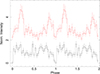 |
Fig. 8. Phase-folded profile (P = 8649 s) in eROSITA data from the observations on November 1–2, 2019 (black profile, reference epoch MJD 58787.991(1), 1σ c.l.) and on November 19, 2019 (red profile, shifted on the y-axis for better visualization). The latter has also been arbitrarily shifted along the x-axis to align the eclipse phase. |
5. Discussion
5.1. The CV W2 in 47 Tuc
This work attempts at ascertaining the nature of the CV W2 in the Galactic GC 47 Tuc. To do so, we carried out a comprehensive spectral and temporal analysis, using all available data sets of the Chandra Data Archive and six eROSITA EDR observations.
We found that the X-ray spectrum of the source can be described equally well using three different models: a power law, a thermal bremsstrahlung, and an optically thin thermal plasma (vmekal). All fits need to include the absorption of the interstellar medium, in excess of ∼1 × 1021 cm−2. The power law model returned a best-fit photon index of Γ = 1.55, while the thermal models resulted in the best-fit temperatures of kT = 10 keV. The latter result is in agreement with those of Heinke et al. (2005) for the 2002 data set (ObsIDs. 2735–8, 3384–7), but not for the 2000 one (ObsIDs. 78, 953–6), which had a higher temperature of the vmekal model. However, it has to be noted that we only used one (ObsID. 955) out of the five 2000 observations to determine the best-fit parameters, which resulted consistent with those of the 2002 data sets.
The inferred unabsorbed fluxes are almost all consistent with each other within uncertainties, resulting in luminosities around the average value of 1.3 × 1032 erg s−1 (Fig. 3), typical of magnetic CVs (e.g. Mukai 2017). In the latest observations (ObsIDs. 26229 and 26286), both taken in 2022, the source appears to have weakened, with a luminosity of 5 × 1031 erg s−1 for ObsID. 26229 and an upper limit of 7 × 1031 erg s−1 for ObsID. 26286.
The period P = 8649 s found by Israel et al. (2016) for the epochs 2000 and 2002 is confirmed also for the observations taken in 2014–15. The presence of a ∼8 min eclipse strongly indicates that this period can be ascribed to the orbital period of the system, placing W2 among the CVs in the period-gap. The eclipse was also confirmed by Rivera Sandoval et al. (2018) in HST data (in the red filter R625).
This is the first time that the source is detected using eROSITA data. Although W2 falls within the dense central region of 1.7′ that eROSITA cannot spatially resolve, we detected the same eclipse profile from the source events extracted from a 15″-radius circular region. The folded eROSITA light curves resemble those of Chandra (cf. e.g. Figs. 6 and 8), hence confirming the identification of W2.
Our analysis did not detect (above the 3.5σ threshold) any other periodicity, neither in Chandra nor in eROSITA data. The detection of the 3846.15 s modulation of Bao et al. (2023) can be probably attributed to the different approach (peak-removal of the fundamental and first harmonic of the orbital period) adopted by the authors. Our in-depth analysis of the candidate signal identified by Bao et al. (2023) shows that this modulation is unrelated to the source and/or not coherent (see Fig. 5), indicating that it is not the spin period of the WD. Moreover, we note that the power spectrum shows an excess of power in the frequency range 1 − 4 × 10⁻⁴ Hz, with several peaks below the detection threshold of 3.5σ. Epoch-folding at each of these individual peaks lead to all sort of sinusoidal profiles. Due to the lack of detection of other significant periodicities, we classify the source as a candidate polar CV, rather than an IP.
The source displays a double-humped phase-folded profile, which is also sometimes observed in polar CVs, as seen for example in AM Her (Heise et al. 1985) and V496 UMa (Kennedy et al. 2022). This profile shape is typically attributed to the emission from both magnetic poles of the WD, with one being more intense than the other, due to the inclination at which the WD is observed. Concerning W2, the energy-resolved folded light curves of the 2002 data sets (e.g. Fig. 7) show similar amplitudes of the two peaks at hard energies, while they are unequal at soft energies. This would suggest that the less active pole is harder than the main pole. The hardness ratio of the source does not give further information, being constant within the error bars. The high cycle-to-cycle variability (Fig. 6), despite no significant changes in the X-ray flux (Fig. 3), would point to a behaviour typical of magnetic CVs of the polar type, as observed for instance for the eclipsing polars 2PBC J0658.0−1746 (Bernardini et al. 2019) or 3XMM J00511.8+634018 (Schwope et al. 2020), which also fall in the period gap.
5.2. The CV populations in GCs
47 Tuc has the highest number of CVs among all Galactic GCs, with a total of 43 CVs and candidate CVs identified so far in HST optical and NUV data (Rivera Sandoval et al. 2018). Among them, several have also been detected and identified in X-rays, thanks to Chandra and eROSITA data (Edmonds et al. 2003a,b; Heinke et al. 2005; Bao et al. 2023; Saeedi et al. 2022). For instance, the most recent work claimed 11 X-ray CVs in the cluster, identifying the CVs based on their periodic signals (Bao et al. 2023).
We confirm that W2 has the second shortest orbital period (∼2.4 h) of all the X-ray CVs in the cluster. 4 out of the 11 CVs have periods within the period gap, close to the ratio for the CVs in the Galaxy bulge, but higher than that for CVs in the solar neighbourhood (20% and 8%, respectively, as reported by Bao et al. 2023). However, it should be noted that the period gap for magnetic CVs is much less marked than that of non-magnetic systems (Webbink & Wickramasinghe 2002). Remarkably, as noted by Bao et al. (2023), in 47 Tuc all the CVs in the period gap are located within the half-light radius (3.17′) and the core radius (0.36′) of the cluster, while longer-period CVs are more centrally concentrated and are found within the core radius. Moreover, no known CV in the GC has a period below the period gap, and the majority of them show longer periods than those of the CVs in the Galaxy bulge and solar neighbourhood. These peculiarities would suggest different formation channels for the GC CVs compared to those in the Galactic bulge and the solar neighbourhood, contributing to the idea that dynamical encounters may have played a significant role in the GC history (e.g. Belloni et al. 2019). This might be especially true for those CVs outside the core radius, such as W2, although a selection bias cannot be entirely excluded (CVs below the period gap are generally less bright). However, observational biases might be present towards the brightest X-ray CVs (i.e. magnetic CVs), which appear to be more abundant in GCs than non-magnetic CVs. Whether this is true or not is still a matter of debate (Knigge 2012; Belloni & Rivera 2021).
Apart from 47 Tuc, three other GCs have a high number of hosted CVs: NGC 6397, NGC 6752, and ω Cen (see Belloni & Rivera 2021, for a review). All these GCs show a bi-modal distribution of the faintest and the brightest CVs when observed in X-rays. However, while in core-collapsed GCs this distribution persists also in optical, in non-core-collapsed GCs, like 47 Tuc, there is no evidence of bimodality at optical wavelengths. Another difference between these GCs lies in the spatial distribution of their CVs. In NGC 6397 and NGC 6752 the bright CVs are concentrated more towards the centre than faint CVs. The same holds for ω Cen, though less evident. Instead, in 47 Tuc CVs are uniformly distributed. This difference can be due to the evolution and relaxation time of the cluster. Nonetheless, with a LX ∼ 1032 erg s−1, W2 is among the brightest CVs in all the aforementioned GCs. This is consistent with its magnetic nature, as magnetic CVs are typically brighter (e.g. Mukai 2017).
6. Conclusions
We investigated the nature of the CV W2 in the Galactic GC 47 Tuc. The source shows characteristics which are common among magnetic CVs: a luminosity of ∼1032 erg s−1, a temperature of 10 keV, and an orbital period of 8649 s (2.4 h). The flux of the source is found to be constant in almost all Chandra observations, taken in 2000, 2002, 2014–15, and 2022. In the latest 2022 observation, W2 is not detected, but the upper limit on its flux is consistent with the previous observation in the same epoch. Our search for pulsations confirms the previous orbital period and finds no other significant signal. The source is also detected for the first time in eROSITA data and the same orbital period is recovered. This source has been proposed to have a second, shorter period of 3846 s, indicating that it might be an asynchronous magnetic CV of the IP type. However, our analysis does not confirm the presence of this second period, based also on the low coherence of the candidate signal which is inconsistent with being originated by a spin modulation. Instead, the cycle-to-cycle variability of the amplitude at the 2.4 h period, as well as its X-ray luminosity, suggests that it is a polar.
A list of Milky Way GCs can be found at https://physics.mcmaster.ca/~harris/mwgc.dat
Acknowledgments
This research is based on data obtained from the Chandra Data Archive and has made use of the software package CIAO provided by the Chandra X-ray Center (CXC). The eROSITA data shown here were processed using the eSASS software system developed by the German eROSITA consortium. The authors thank the anonymous referee whose constructive feedback significantly improved the scientific quality and the readability of this paper. RA and GLI acknowledge financial support from INAF through grant “INAF-Astronomy Fellowships in Italy 2022 – (GOG)”. MI is supported by the AASS Ph.D. joint research programme between the University of Rome “Sapienza” and the University of Rome “Tor Vergata”, with the collaboration of the National Institute of Astrophysics (INAF). PE and GLI acknowledge financial support from the Italian Ministry for University and Research, through the grants 2017LJ39LM (UNIAM) and 2022Y2T94C (SEAWIND), and from INAF through LG 2023 BLOSSOM. DdM acknowledges support from INAF Astrofund2022. RA and NW are grateful for support provided by the CNES for this work.
References
- Arnaud, K. A. 1996, ASP Conf. Ser., 101, 17 [Google Scholar]
- Bachetti, M. 2018, Astrophysics Source Code Library [record ascl:1805.019] [Google Scholar]
- Bao, T., Li, Z., & Cheng, Z. 2023, MNRAS, 521, 4257 [NASA ADS] [CrossRef] [Google Scholar]
- Baumgardt, H., & Vasiliev, E. 2021, MNRAS, 505, 5957 [NASA ADS] [CrossRef] [Google Scholar]
- Belloni, D., & Rivera, L. 2021, The Golden Age of Cataclysmic Variables and Related Objects V, 13 [Google Scholar]
- Belloni, D., Giersz, M., Rivera Sandoval, L. E., Askar, A., & Ciecielåg, P. 2019, MNRAS, 483, 315 [NASA ADS] [CrossRef] [Google Scholar]
- Bernardini, F., de Martino, D., Mukai, K., Falanga, M., & Masetti, N. 2019, MNRAS, 489, 1044 [Google Scholar]
- Bhattacharya, S., Heinke, C. O., Chugunov, A. I., et al. 2017, MNRAS, 472, 3706 [NASA ADS] [CrossRef] [Google Scholar]
- Brunner, H., Liu, T., Lamer, G., et al. 2022, A&A, 661, A1 [NASA ADS] [CrossRef] [EDP Sciences] [Google Scholar]
- Buccheri, R., Bennett, K., Bignami, G. F., et al. 1983, A&A, 128, 245 [NASA ADS] [Google Scholar]
- Chen, S., Richer, H., Caiazzo, I., & Heyl, J. 2018, ApJ, 867, 132 [Google Scholar]
- Edmonds, P. D., Gilliland, R. L., Heinke, C. O., & Grindlay, J. E. 2003a, ApJ, 596, 1197 [NASA ADS] [CrossRef] [Google Scholar]
- Edmonds, P. D., Gilliland, R. L., Heinke, C. O., & Grindlay, J. E. 2003b, ApJ, 596, 1177 [NASA ADS] [CrossRef] [Google Scholar]
- García-Berro, E., Torres, S., Althaus, L. G., & Miller Bertolami, M. M. 2014, A&A, 571, A56 [NASA ADS] [CrossRef] [EDP Sciences] [Google Scholar]
- Gregory, P. C., & Loredo, T. J. 1992, ApJ, 398, 146 [NASA ADS] [CrossRef] [Google Scholar]
- Grindlay, J. E., Heinke, C., Edmonds, P. D., & Murray, S. S. 2001, Science, 292, 2290 [NASA ADS] [CrossRef] [Google Scholar]
- Heinke, C. O., Grindlay, J. E., Edmonds, P. D., et al. 2005, ApJ, 625, 796 [NASA ADS] [CrossRef] [Google Scholar]
- Heise, J., Brinkman, A. C., Gronenschild, E., et al. 1985, A&A, 148, L14 [NASA ADS] [Google Scholar]
- Israel, G. L., & Stella, L. 1996, ApJ, 468, 369 [Google Scholar]
- Israel, G. L., Esposito, P., Rodríguez Castillo, G. A., & Sidoli, L. 2016, MNRAS, 462, 4371 [Google Scholar]
- Kennedy, M. R., Littlefield, C., & Garnavich, P. M. 2022, MNRAS, 513, 2930 [NASA ADS] [CrossRef] [Google Scholar]
- Knigge, C. 2012, Mem. Soc. Astron. It., 83, 549 [NASA ADS] [Google Scholar]
- Lugaro, M., D’Orazi, V., Campbell, S. W., et al. 2013, Mem. Soc. Astron. It., 84, 109 [NASA ADS] [Google Scholar]
- Marks, M., & Kroupa, P. 2010, MNRAS, 406, 2000 [NASA ADS] [Google Scholar]
- Mewe, R. 1991, A&ARv, 3, 127 [Google Scholar]
- Meylan, G., & Heggie, D. C. 1997, A&ARv, 8, 1 [NASA ADS] [CrossRef] [Google Scholar]
- Mukai, K. 2017, PASP, 129, 062001 [Google Scholar]
- Pooley, D., & Hut, P. 2006, ApJ, 646, L143 [NASA ADS] [CrossRef] [Google Scholar]
- Pooley, D., Lewin, W. H. G., Anderson, S. F., et al. 2003, ApJ, 591, L131 [NASA ADS] [CrossRef] [Google Scholar]
- Predehl, P., Andritschke, R., Arefiev, V., et al. 2021, A&A, 647, A1 [EDP Sciences] [Google Scholar]
- Rivera Sandoval, L. E., van den Berg, M., Heinke, C. O., et al. 2018, MNRAS, 475, 4841 [NASA ADS] [CrossRef] [Google Scholar]
- Saeedi, S., Liu, T., Knies, J., et al. 2022, A&A, 661, A35 [NASA ADS] [CrossRef] [EDP Sciences] [Google Scholar]
- Schwope, A. D., Worpel, H., Webb, N. A., Koliopanos, F., & Guillot, S. 2020, A&A, 637, A35 [NASA ADS] [CrossRef] [EDP Sciences] [Google Scholar]
- Simunovic, M., Puzia, T. H., Miller, B., et al. 2023, ApJ, 950, 135 [NASA ADS] [CrossRef] [Google Scholar]
- Strader, J., Chomiuk, L., Maccarone, T. J., et al. 2012, ApJ, 750, L27 [NASA ADS] [CrossRef] [Google Scholar]
- Thompson, I. B., Udalski, A., Dotter, A., et al. 2020, MNRAS, 492, 4254 [Google Scholar]
- Thygesen, A. O., Sbordone, L., Andrievsky, S., et al. 2014, A&A, 572, A108 [NASA ADS] [CrossRef] [EDP Sciences] [Google Scholar]
- Truemper, J. 1982, Adv. Space Res., 2, 241 [Google Scholar]
- Verner, D. A., Ferland, G. J., Korista, K. T., & Yakovlev, D. G. 1996, ApJ, 465, 487 [Google Scholar]
- Webbink, R. F., & Wickramasinghe, D. T. 2002, MNRAS, 335, 1 [NASA ADS] [CrossRef] [Google Scholar]
- Weisskopf, M. C., Tananbaum, H. D., Van Speybroeck, L. P., & O’Dell, S. L. 2000, SPIE Conf. Ser., 4012, 2 [Google Scholar]
- Wilms, J., Allen, A., & McCray, R. 2000, ApJ, 542, 914 [Google Scholar]
- Zoccali, M., Renzini, A., Ortolani, S., et al. 2001, ApJ, 553, 733 [NASA ADS] [CrossRef] [Google Scholar]
Appendix A: Chandra observations of 47 Tuc
Log of Chandra observations in chronological order.
Appendix B: Best-fit results
The following tables show the best-fit parameters obtained from fitting the seven data sets 955, 2735, 2736, 2737, 2738, 15747, 16527 individually (columns 2–6) and from imposing the same local absorption  (columns 7–8).
Best-fit values of the seven data sets 955, 2735, 2736, 2737, 2738, 15747, 16527 with the power law model.
As before, for the thermal Bremsstrahlung model.
As before, for the vmekal model.
All Tables
Best-fit values of the seven data sets 955, 2735, 2736, 2737, 2738, 15747, 16527 with the power law model.
All Figures
|
Fig. 1. Chandra (left panel, ObsID. 2735) and eROSITA (right panel, 1−2 Nov. 2019 observations) images of the field of view of 47 Tuc. Solid and dashed circles represent the source and background extraction regions for W2, respectively, for Chandra (red) and eROSITA (blue). The black circle encloses the inner region of the cluster excluded in the eROSITA analysis of Bao et al. (2023) and has a radius of 1.7′. The box in the bottom left corner is a close-up of the eROSITA source region as seen by Chandra, to show the X-ray sources that are blended with W2 in the eROSITA image. |
| In the text | |
|
Fig. 2. Summed spectra from all the Chandra data sets in which the source was detected, together with the best-fit power-law model (top panel), and residuals in units of |
| In the text | |
|
Fig. 3. Light curve of W2. Empty data points are for those observations with exposures shorter than the orbital period; the black arrow represents the upper limit at 90% c.l. on the luminosity of the latest Chandra observation (ObsID. 26286); the grey dotted line and area represents the average luminosity of the source and its uncertainty at 90 % c.l., respectively. |
| In the text | |
|
Fig. 4. Results of the pulsation searches in Chandra data of W2. Left panel: power density spectrum (PDS) in the 0.2−10 keV energy range by using the 2002 datasets 2735–8 and one single interval. The 3.5σ detection threshold is also shown and marked by the blue solid line. The PDS is complex and only one peak is above the threshold, corresponding to the harmonic of the 8649 s period (both the fundamental and the harmonic are marked by I17 and 1/2P I17, respectively). The period suggested by Bao et al. (2023) is indicated as B23. Right: |
| In the text | |
|
Fig. 5. Phase-fitting of the 3846.15 s period of Bao et al. (2023), where each data point corresponds to a duration of one orbital cycle (i.e. 8649 s). The phases are highly scattered up to almost 40% of the period, suggesting that this period is spurious and/or not coherent. The black solid and stepped lines mark the best fit linear component and its 1σ uncertainty, respectively. |
| In the text | |
|
Fig. 6. Chandra ACIS eclipse profiles of W2, folded to the best period of P = 8649 s. Top panel: profiles for the three different epochs where the modulation was detected: 2000 (red line and filled circles), 2002 (black lines), and 2014 (blue line and filled squares). A correction of about 20% was applied to the 2000 datasets in order to take into account the difference in CCD efficiency between ACIS-I and ACIS-S. We used the reference epoch MJD 52551.999(1) (1σ c.l.) for the 2002 datasets, while the 2000 and 2014 light curves have been arbitrarily shifted along the x-axis in order to align the minima, corresponding to the 8-min eclipse. All light curves have 20 phase-bins of ∼432 s duration each. Bottom panel: folded light curves of the four longest observations, carried out in 2002 a few days apart from each other. From top to bottom: ObsID. 2735, 2736, 2737 and 2738. The profiles are complex and variable on time scales of less than a day. |
| In the text | |
|
Fig. 7. Energy-resolved profiles of the summed 2002 data sets, in units of normalised intensity, for the following energy ranges: 0.3–2 keV (first panel), 2–6 keV (second panel), 6–10 keV (third panel). Bottom panel: hardness ratio (2–6 keV)/(0.3–2 keV). |
| In the text | |
|
Fig. 8. Phase-folded profile (P = 8649 s) in eROSITA data from the observations on November 1–2, 2019 (black profile, reference epoch MJD 58787.991(1), 1σ c.l.) and on November 19, 2019 (red profile, shifted on the y-axis for better visualization). The latter has also been arbitrarily shifted along the x-axis to align the eclipse phase. |
| In the text | |
Current usage metrics show cumulative count of Article Views (full-text article views including HTML views, PDF and ePub downloads, according to the available data) and Abstracts Views on Vision4Press platform.
Data correspond to usage on the plateform after 2015. The current usage metrics is available 48-96 hours after online publication and is updated daily on week days.
Initial download of the metrics may take a while.