| Issue |
A&A
Volume 689, September 2024
|
|
|---|---|---|
| Article Number | A126 | |
| Number of page(s) | 19 | |
| Section | Astrophysical processes | |
| DOI | https://doi.org/10.1051/0004-6361/202449465 | |
| Published online | 11 September 2024 | |
Non-resonant relaxation of rotating globular clusters
1
Institut d’Astrophysique de Paris, CNRS and Sorbonne Université, UMR 7095, 98 bis Boulevard Arago, 75014 Paris, France
2
Department of Physics and Astronomy, The University of North Carolina at Chapel Hill, Chapel Hill, NC 27599, USA
3
IPhT, DRF-INP, UMR 3680, CEA, L’Orme des Merisiers, Bât. 774, 91191 Gif-sur-Yvette, France
4
Korea Institute for Advanced Study, 85 Hoegi-ro, Dongdaemun-gu, Seoul 02455, Republic of Korea
Received:
2
February
2024
Accepted:
11
June
2024
The long-term relaxation of rotating, spherically symmetric globular clusters is investigated through an extension of the orbit-averaged Chandrasekhar non-resonant formalism. A comparison is made with the long-term evolution of the distribution function in action space, measured from averages of sets of N-body simulations up to core collapse. The impact of rotation on in-plane relaxation is found to be weak. In addition, we observe a clear match between theoretical predictions and N-body measurements. For the class of rotating models considered, we find no strong gravo-gyro catastrophe accelerating core collapse. Both kinetic theory and simulations predict a reshuffling of orbital inclinations from overpopulated regions to underpopulated ones. This trend accelerates as the amount of rotation is increased. Yet, for orbits closer to the rotational plane, the non-resonant prediction does not reproduce numerical measurements. We argue that this mismatch stems from these orbits’ coherent interactions, which are not captured by the non-resonant formalism that only addresses local deflections.
Key words: diffusion / gravitation / galaxies: kinematics and dynamics
© The Authors 2024
 Open Access article, published by EDP Sciences, under the terms of the Creative Commons Attribution License (https://creativecommons.org/licenses/by/4.0), which permits unrestricted use, distribution, and reproduction in any medium, provided the original work is properly cited.
This article is published in open access under the Subscribe to Open model. Subscribe to A&A to support open access publication.
1. Introduction
Rotation is ubiquitous in stellar systems. In effect, it provides a source of free energy, allowing clusters to efficiently reshuffle their orbital structure towards more likely configurations. Yet, historically, the study of globular clusters has been mainly focused on isotropic, non-rotating, old globular clusters (Aarseth et al. 1974; Spitzer 1975; Cohn 1979; Trager et al. 1995; Miocchi et al. 2013). The reasons behind such simplifications are two-fold: (i) naturally, it is easier numerically and analytically to neglect the effect of rotation; (ii) spherical isotropic models – for example, the King models (King 1966) or the Wilson models (Wilson 1975) – provided a satisfactory zeroth-order description of the main observed dynamical properties of globular clusters (see, e.g., McLaughlin & van der Marel 2005).
The last decade has seen the extraction of new data – for instance, HST (Bellini et al. 2017) and Gaia DR2 (Bianchini 2018; Sollima et al. 2019). These surveys gave the astrophysical community access to numerous and detailed observations of the internal kinematics of several globular clusters of the Milky Way (Bianchini et al. 2013; Fabricius et al. 2014; Watkins et al. 2015; Ferraro et al. 2018; Kamann et al. 2018), as well as a quantification of the degree of velocity anisotropy (Jindal et al. 2019). Using these new data sets, the historical highly symmetric cluster models are not satisfactory anymore.
Therefore, a secular theory that describes the evolution of globular clusters and accounts for their rotation is needed to describe their long-term evolution. In particular, the Fokker-Planck theory was used to probe the impact of rotation of the long-term evolution of such clusters, both before (Einsel & Spurzem 1999) and after (Kim et al. 2002) core collapse. Furthermore, observations show that the angular momentum distribution measured in Galactic clusters retain the signature of their formation process (Lanzoni et al. 2018). While N-body simulations are able to reproduce these results (Tiongco et al. 2016, 2022), the historical context and the complexity of the problem have led to few analytical explorations (Geyer et al. 1983; White & Shawl 1987; Kontizas et al. 1989). These remain scarce even now (see, e.g., Stetson et al. 2019; Rozier et al. 2019; Livernois et al. 2022).
In isolated systems, a non-zero total angular momentum, that is, the presence of rotation, can have a significant impact on the cluster’s long-term evolution, for instance, through the “gravo-gyro catastrophe” (Hachisu 1979; Ernst et al. 2007). This phenomenon has been observed in a range of rotating systems, including gas cylinders (Inagaki & Hachisu 1978; Hachisu 1979), gaseous discs (Hachisu 1982), flattened (quasi-spherical) star clusters (Akiyama & Sugimoto 1989; Einsel & Spurzem 1999; Ernst et al. 2007), and clusters with embedded black holes (BHs) (Fiestas & Spurzem 2010; Kamlah et al. 2022). Let us however note that many of these studies used a rotating King model to study the impact of rotation (see, e.g., Einsel & Spurzem 1999; Varri & Bertin 2012). Therein, changing the amount of rotation impacts the density profile: this makes comparisons amongst different models less clear.
The concurrent occurrence of internal rotation and a spectrum of stellar masses can result in the formation of an oblate core of fast rotating heavy masses (Kim et al. 2004; Tiongco et al. 2021). More precisely, the orbital inclinations of the heaviest stars align with respect to one another, inducing a mass segregation in the distribution of orbital inclinations (Szölgyén et al. 2019). The generally agreed explanation for this phenomenon is resonant relaxation and resonant friction (Rauch & Tremaine 1996; Meiron & Kocsis 2019). While this effect concerns globular clusters, nuclear cluster with a dominant massive BH (Szölgyén & Kocsis 2018; Foote et al. 2020; Gruzinov et al. 2020; Magnan et al. 2022; Ginat et al. 2023) also display this spontaneous alignment.
The objective of this paper is to explore the impact of rotation on the long-term evolution of spherically symmetric globular clusters. To achieve this goal, we extend the orbit average analysis of anisotropic Plummer globular clusters from Tep et al. (2022) to the case of rotating clusters. By performing tailored N-body simulations, we quantify the validity of Chandrasekhar’s non-resonant relaxation (NR) theory (Chandrasekhar 1943), and assess the importance of the gravo-gyro catastrophe as well as that of collective effects (i.e., the self-amplification of the star’s gravitational response, see Heyvaerts 2010).
This paper is organised as follows. In Section 2, we extend the NR theory to rotating clusters. In Section 3, we follow the long-term evolution of a series of rotating clusters using N-body simulations. We study the impact of rotation on core collapse and on the distribution of orbital inclinations. We compare the NR prediction with N-body simulations in Sections 4 (in-plane diffusion) and 5 (out-of-plane diffusion). Finally, we discuss our results in Section 6.
2. Non-resonant relaxation
We consider a self-gravitating globular cluster composed of N stars of individual mass m = M/N, with M the cluster’s total mass. We follow the cluster’s evolution through the total distribution function (DF) in (r, v) space, Frot = Frot(r, v), with r the position and v the velocity. All normalisations are taken to be the same as in Section 2 of Tep et al. (2022), hereafter T22. In addition to quasi-stationarity, we assume the cluster to be spherically symmetric – hence, with planar unperturbed orbits – and in rotation. Since we are interested in orbital distortion, it is convenient to monitor the cluster’s evolution in action space, via Frot = Frot(J), where J = (Jr, L, Lz) are the specific action coordinates. Here, Jr is the radial action, L the norm of the angular momentum vector and Lz its projection along the z-axis. We also introduce the orbital inclination through cos I = Lz/L. Because actions are integrals of motion, we use them to label the cluster’s orbits and track their deformation over time.
The long-term evolution of the cluster’s DF is described by the FP equation (see, e.g., section 7.4 of Binney & Tremaine 2008)
![$$ \begin{aligned} \frac{{\partial } F_{\mathrm{rot}} ({\boldsymbol{J}},t)}{{\partial } t} &\!=\! - \frac{{\partial } }{{\partial } {\boldsymbol{J}}} \!\cdot \! {\boldsymbol{\mathcal{F} }} ({\boldsymbol{J}}) \\&\!=\! - \frac{{\partial } }{{\partial } {\boldsymbol{J}}}\! \cdot \!\bigg [ {\boldsymbol{D}}_{1} ({\boldsymbol{J}}) \, F_{\mathrm{rot}} ({\boldsymbol{J}})\!-\! \frac{1}{2} \frac{{\partial } }{{\partial } {\boldsymbol{J}}} \!\cdot \! \bigg ( {\boldsymbol{D}}_{2} ({\boldsymbol{J}}) \, F_{\mathrm{rot}} ({\boldsymbol{J}}) \bigg ) \bigg ] ,\nonumber \end{aligned} $$](/articles/aa/full_html/2024/09/aa49465-24/aa49465-24-eq1.gif)
with ℱ(J) the action space flux. Therein, we find the first-order diffusion coefficient, D1, and the diffusion matrix, D2. Both of them describe the distortion of orbits in action space. The next two sections briefly describe the main steps needed to compute this diffusion flux in Equation (1).
2.1. Local velocity deflection coefficients
Let us consider a test star of mass m and velocity v. As a result of the cluster’s finite number of constituents, this test star is subject to perturbations around its mean field trajectory, driving an irreversible diffusion of its velocity. We call this long-term relaxation process, sourced by successive, uncorrelated pairwise deflections, the NR relaxation. Following Appendix L of Binney & Tremaine (2008) (p. 836), the corresponding local velocity deflection coefficients generically read
where 1 ≤ i, j ≤ 3 run over the three directions of the coordinate system. We also defined A = 4πmG2lnΛ and the relative velocity w = v − v′. Here, lnΛ stands for the Coulomb logarithm, set to Λ = 0.11N as is usual for single-mass globular clusters (Giersz & Heggie 1994; Heggie & Hut 2003). In principle, the rewriting of these expressions using Rosenbluth potentials is feasible, as outlined by Rosenbluth et al. (1957). Such a program, in a non-rotating but anisotropic cluster, was pursued in T22.
In Appendix A, we improve upon this approach in the context of rotating clusters. In particular, we show how a rewriting rather based on Equations (2) improves the numerical stability and ensures the positivity of the second-order diffusion coefficients. More precisely, we write Equations (2) as
where Δv∥ (resp. Δv⊥) is the local velocity deflection along (resp. perpendicular to) the test star’s trajectory and we have used polar coordinates (w, ϑ, ϕ) with the z-axis parallel to v (see Fig. A.1). Appendix A.1 also details the arguments at which the DF,  , must be evaluated.
Equation (3) is one of the main results of the present work. In particular, Equation (3) possesses a few key advantages compared to the expressions given in Equations (3) of T22, which are recovered by the present approach: (i) no integrable singular denominators remain; (ii) no gradients of Frot are required during the computation; (iii) the positivity of the second-order coefficients is ensured; (iv) this equation applies to a wider range of clusters. Ultimately, Equation (3) compactly accounts for all the two-body deflections from the cluster’s stars onto the test star.
2.2. Orbit average and secular evolution
Because we are interested in the diffusion of orbits, we must consider the effect of NR on orbital invariants, namely the energy E and the angular momenta L and Lz. In Appendix B, we expand upon T22 and detail how the local diffusion coefficients in (E, L, Lz) may be computed from the local velocity coefficients given in Equation (3).
Once the local diffusion coefficients are known, they can be averaged along the unperturbed mean field orbit of the test star. At this stage, our accounting of rotation adds some complexity. Indeed, the orbit average now involves an intricate two-dimensional integral spanning the radial range of the test orbit (r ∈ [rp, ra]) and its angular phase (φ ∈ [0, 2π]) within the orbital plane. This is illustrated in Fig. 1.
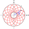 |
Fig. 1. Illustration of the orbit average in physical space. The test star (in black, part of whose orbit is shown in red) is averaged over all its available positions in its orbital plane, within the radial range of the orbit (r ∈ [rp, ra]) and its angular range (φ ∈ [0, 2π]), weighted by the surface density Ωr/(2π2|vr|). Here, the frame is that of the right panel of Fig. A.2. |
In practice, computing the orbit average diffusion coefficients involves computing expressions of the form
where X runs over all the diffusion coefficients to compute, that is, runs over singlets and pairs from {E, L, Lz}. Here, Ωr is the radial frequency and vr the radial velocity that is evaluated along the mean field orbit. We refer to Appendix C for detailed expressions. In particular, in Appendix C.1, we show how the angular average can be performed explicitly for some classes of rotating models. And, in Appendix C.2, we use the same approach as in appendix F2 of T22 to compute the radial average using a stable numerical integration scheme.
The final stage of the calculation is to convert the orbit-averaged diffusion coefficients in (E, L, Lz) into ones in J = (Jr, L, Lz). This is rather straightforward, as detailed in Appendix D. Lastly, these diffusion coefficients are those used to evaluate the FP Equation (1). Along the same lines, one can similarly describe the dynamics within the coordinates Jc = (Jr, L, cos I).
3. Long-term relaxation
We wish to study the impact of rotation on the long-term evolution of rotating, spherically symmetric1, anisotropic clusters. In this first section, we focus on direct N-body simulations to get some insight on the dynamics at play. We detail the corresponding numerical setup in Appendix E.
First, let us describe the classes of clusters considered. The in-plane distribution of orbits (i.e., when projecting in the (Jr, L) space) follows the same Plummer DFs (see, e.g., Dejonghe 1987) as in Section 3.1 of T22. Velocity anisotropy is encoded with the dimensionless parameter q, with q = 0 corresponding to an isotropic distribution, and q > 0 (resp. q < 0) associated with radially (resp. tangentially) anisotropic velocity distributions.
Let us introduce rotation in these models, while leaving the mean potential invariant. To do so, we follow the Lynden-Bell daemon (LBD) (Lynden-Bell 1960) and consider
![$$ \begin{aligned} F_{\mathrm{rot}}({\boldsymbol{J}}) = F_{\mathrm{tot}}(J_{\mathrm{r}},L) \, \big (1+\alpha \,{\mathrm{sgn}}[L_{z}/L] \big ), \end{aligned} $$](/articles/aa/full_html/2024/09/aa49465-24/aa49465-24-eq7.gif)
where Ftot(Jr, L) is the non-rotating DF and α a dimensionless parameter between 0 and 1. Physically, this parameter corresponds to converting a fraction α of retrograde orbits (Lz < 0) into prograde orbits (Lz > 0). Importantly, since Lz ↦ sgn[Lz/L] is an odd function, we stress that Ftot and Frot generate the exact same potential.
When considering orbital inclinations via Jc = (Jr, L, cos I) (see Appendix D.3), the LBD yields the DF in Jc space2
![$$ \begin{aligned} F ({\boldsymbol{J}_{\mathrm{c}}}) = L \, F_{\mathrm{tot}} (J_{\mathrm{r}} , L) \, \big ( 1 \!+\! \alpha \, {\mathrm{sgn}} [\cos I] \big ) . \end{aligned} $$](/articles/aa/full_html/2024/09/aa49465-24/aa49465-24-eq8.gif)
Integrating this equation over cos I, one recovers the reduced DF in (Jr, L), F(Jr, L) = 2LFtot(Jr, L), used to describe non-rotating clusters (see, e.g., Hamilton et al. 2018).
3.1. Sphericity of the cluster
The NR theory presented in Section 2 assumes that the cluster remains spherically symmetric throughout. However, Rozier et al. (2019) showed that (sufficiently) rotating clusters can harbour unstable modes (see, e.g., Fig. 8 therein). To avoid this complication, we restricted ourselves to (linearly) stable rotating clusters, that is, clusters that would remain spherically symmetric.
To probe the conservation of spherical symmetry, we investigateed the “sphericity”, h, of clusters, as defined in Appendix F in terms of the eigenvalue ratio of the density-weighted inertia tensor. This is illustrated in Fig. 2.
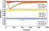 |
Fig. 2. Sphericity, h, of a sample of rotating anisotropic clusters, as defined in Appendix F, from N-body simulations for N = 105. Each case has been averaged over 50 realisations. We represent radially anisotropic clusters (q = 1) in red, isotropic clusters (q = 0) in yellow, and tangentially anisotropic ones (q = − 6) in blue. For each anisotropy, we consider three rotating parameters α = 0.1, 0.25, 0.5 (ordered from dark to light colors). In agreement with Rozier et al. (2019), some of these clusters are unstable – namely (q, α) = (1, 0.5), and in a smaller fashion (q, α) = (1, 0.25) – while the others are linearly stable and remain spherically symmetric. |
Except for the radially-anisotropic and rapidly-rotating cluster (q, α) = (1, 0.5), all clusters remain approximately spherical. This is in agreement with the measurements from Rozier et al. (2019), as this particular cluster falls into the region of linear instability. Therefore, we shall focus our interest on parameters (q, α) for which the clusters remain spherically symmetric.
3.2. The gravo-gyro catastrophe
The typical relaxation timescale of a globular cluster can be estimated through the half-mass relaxation time (see, e.g., Section 14 of Heggie & Hut 2003, for more details), defined by

with rh the half-mass radius. For a cluster with N = 105 stars, this yields trh = 994 HU, where HU stands for the Hénon units (Heggie & Mathieu 1986) in which G = M = Rv = 1, with Rv the virial radius3. In practice, with N = 105 running a numerical simulation up to t ∼ trh took about one day of computation, see Appendix E. In Breen et al. (2017), core collapse occurs at t ∼ 17trh for an isotropic cluster (see Table 1 therein for the dependence with respect to velocity anisotropy). Hence, integrating clusters with N = 105 up to core collapse is not reasonably feasible. In this section we therefore scaled down the size of the clusters to N = 104 stars. In that case, trh = 132 HU, and core collapse was numerically reached in about ten hours. Since we focused on measuring the core radius – a very integrated quantity – the quality of the numerical measurements was not too much degraded by this use of a smaller value for N. In practice, measurements were averaged over 50 runs.
Figure 3 represents the time evolution of the averaged core radius, Rc, defined as (see, e.g., Breen et al. 2017; T22)
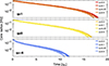 |
Fig. 3. Core radius as a function of time, as measured in N-body simulations, with trh defined in equation (7). Each case has been averaged over 50 realisations with N = 104. Increasing the rotation strength α slightly reduces the time of core collapse. Nevertheless, the impact of rotation (i.e. the gravo-gyro catastrophe) is surely not as pronounced as what was observed in, e.g., Einsel & Spurzem (1999). |
where ri is the radial position of star i and ρi an estimator of the density at ri, as defined in NBODY6++GPU (Wang et al. 2015). For the usual sets of anisotropies and rotations (q = 1, 0, −6 and α = 0, 0.1, 0.25, 0.5).
Interestingly, for these rotating clusters, the impact of rotation is definitely not as important as the one reported in Einsel & Spurzem (1999) in rotating King models (see Figure 2 therein). Appendix G reproduces the main parameters characterising these models. For example, in Einsel & Spurzem (1999), assuming W0 = 6.0, a non-rotating King cluster collapses at t ∼ 12trh, while a rotating one, with ω0/Ω0 = 0.4, can collapse as early as t ∼ 9trh. Here, for Plummer spheres, we do not find any such stark impact of rotation.
Nonetheless, Figure 3 does not contradict the measurements from Einsel & Spurzem (1999). Indeed, the parameters ω0 (King) and α (Plummer) do not parametrise rotation in the same way. As Einsel & Spurzem (1999) varies ω0, the mean density profile gets modified. Indeed, the rotating DF of the King model (Equation G.1) cannot be decomposed into a fixed, rotation-free even part, and an odd part in Lz (see, e.g., Dejonghe 1986). As such, we argue that the LBD approach ensures a fairer comparison between models to isolate the distinctive impact of rotation.
Of course, to better assess the universality of these observations, it would be worthwhile to perform similar experiments with other parametrisations for the rotation (see Appendix K). This is left for future investigations.
3.3. In-plane vs out-of-plane diffusion
Using once again N-body simulations with N = 104 stars, let us finally investigate the typical features of the in-plane diffusion (i.e. relaxation in (Jr, L)) and out-of-plane diffusion (i.e. relaxation in cos I).
First, Fig. 4 reports on the time evolution of the DF in L, that is, the in-plane relaxation of the distribution of angular momenta. There, we recover the imprints of core collapse visible through the slow overall contraction of the distribution. But importantly, we clearly note that rotation only (very) weakly impacts this relaxation.
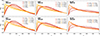 |
Fig. 4. Evolution of the angular momentum DF, F(L), as measured in N-body simulations with N = 104, with trh defined in Equation (7). For each parameter, the latest time is close to the time of core collapse. Each panel is averaged over 50 realisations. Here, F(L) redistributes towards lower angular momenta, with details depending on the initial velocity anisotropy. Rotation does not impact strongly the in-plane relaxation. |
We can now compare this relaxation with the out-of-plane one. Figure 5 reports on the time evolution of the DF in cos I. As could have been expected, the clusters tend towards smoother distribution of inclinations, meaning that relaxation tends to erase discontinuities. The sharp discontinuity at cos I = 0 has already been washed away after 1 trh, regardless of the initial amplitude of the discontinuity. We refer to Appendix K.2 for a comparison of the early relaxation between a discontinuous and a smooth distribution of orbital inclinations. Note that the redistribution of prograde and retrograde orbits observed in Fig. 5 does not conflict with the conservation of the cluster’s total angular momentum. Indeed, the average of cos I = Lz/L is not constrained by any global invariance, contrary to Lz. As such, even if the number of particles with positive and negative cos I (hence Lz) changes, the conservation of the total angular momentum is ensured by a modulation of the norm of each star’s angular momentum vector.
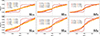 |
Fig. 5. Same as Fig. 4 but for the DF in orbital inclinations, F(cos I). The out-of-plane relaxation does not depend much on the initial velocity anisotropy. As time evolves, the discontinuity of the LBD (Equation (5)) at cos I = 0 is (rapidly) washed out. |
Comparing Figs. 4 and 5 shows that orbital inclinations relax much faster than angular momenta. This is a point already raised in Rauch & Tremaine (1996) (Fig. 2 therein). In particular, they showed in their Section 1.4 that the long-term relaxation of E and L in spherical potential was driven by the NR theory, whereas that of the angular momentum vector L – and thus Lz – was subject to an enhanced relaxation. This out-of-plane relaxation is driven by coherent torques between orbits and is coined vector resonant relaxation (VRR).
4. In-plane diffusion
Assuming that the cluster’s relaxation is driven by local pairwise deflections, its long-term evolution is described by the FP Equation (1). While this equation formally describes the evolution in 3D action space, it is convenient to study relaxation in two-dimensional projections, in particular to improve the signal-to-noise ratio. Yet, such a projection comes at the cost of more intricate theoretical predictions, that require additional integrations along some third action. In this section, following the same approach as in T22, we first focus on in-plane relaxation, that is, relaxation occurring in (Jr, L). Our goal is to compare quantitatively the N-body measurements with the NR prediction.
4.1. N-body measurements
The onset of core collapse is illustrated in Fig. 6 for clusters with N = 105 stars. As in Fig. 3, we recover that rotation does not really impact the rate of core collapse in these linearly stable clusters. Conversely, when the clusters are unstable, such as for (q, α) = (1, 0.5) (see Fig. 2), we find numerically (not reported in Fig. 6) that the clusters flatten and that relaxation is accelerated.
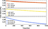 |
Fig. 6. Initial evolution of the core radius in clusters with N = 105 stars, as measured in N-body simulations. We use that same convention as in Fig. 2. Interestingly, in these stable clusters, rotation only weakly affects the core contraction. |
To probe more precisely relaxation, let us now measure the relaxation rate, ∂F/∂t, in (Jr, L). This is presented in Fig. 7 with details spelled out in Appendix E. Even in the presence of rotation, we recover the same result as in T22, namely all clusters seem to isotropise toward an in-plane DF depending only on energy. Indeed, in radially anisotropic clusters, relaxation depletes radial orbits. And the converse holds for tangentially anisotropic clusters. Importantly, the amount of rotation, α, has no significant impact on the geometry of the in-plane diffusion. Increasing α only (very) weakly accelerates the in-plane relaxation. This is in concordance with the slightly shorter core collapse time observed in Fig. 3.
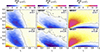 |
Fig. 7. Relaxation rate, ∂F/∂t, in (Jr, L) for various velocity anisotropies q (left to right) and rotation parameters α (top and bottom), as measured in N-body simulations. The overall amplitude of the in-plane relaxation rate depends on q, but only very weakly on α. |
4.2. Non-resonant prediction
Let us now compute the NR prediction for the relaxation rate in (Jr, L). This prediction was numerically very intensive and required the evaluation of five embedded integrals, as demonstrated in Appendices A and H. Importantly, we stress that in the present case, the LBD (Equation (5)) allowed us to analytically perform the angular part of the orbit average (Equation (4)). This helped reducing the computation time. We refer to Appendix C.1 for details.
The relaxation rate, ∂F/∂t in (Jr, L), presented in Fig. 8 for various anisotropies and rotations, suggests once again an orbital reshuffling toward isotropisation. In addition, increasing the rotation parameter α only very weakly increases the relaxation rate in (Jr, L), while barely impacting the structures observed in the non-rotating case.
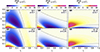 |
Fig. 8. Relaxation rate, ∂F/∂t, in (Jr, L) as in Fig. 7, but here from the NR theory. The prediction matches the N-body measurements from Fig. 7, up to an overall prefactor that depends on q, and (very) weakly on α. |
When comparing the N-body measurements (Fig. 7) with the NR prediction (Fig. 8), the NR theory successfully recovers the in-plane relaxation of stable rotating clusters: both figures exhibit strikingly similar structures in action space. We obtain results for the non-rotating case that are in agreement with T22. Yet, even though amplitudes in both approaches are comparable, there is still a (slight) overall prefactor mismatch. The inclusion of rotation has little impact on this mismatch. A more quantitative comparison would require performing (many) more N-body runs, as well as a more precise measurement of the relaxation rate. This would be no light undertaking, and will be the subject of future works.
5. Out-of-plane diffusion
Because they rotate, the present clusters also undergo some out-of-plane diffusion, namely relative to the orbital inclinations cos I. In this section, we focus on relaxation in (Jr, cos I), and we refer to Appendix J for a similar investigation in (L, cos I).
5.1. N-body measurements
The relaxation rates in N-body simulations are presented in Fig. 9. As expected, in the absence of rotation (top row), the relaxation is independent of cos I, and the distribution of orientations remains uniform.
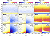 |
Fig. 9. Relaxation rate, ∂F/∂t, in (Jr, cos I) for various anisotropies q (left to right) and rotation α (from top to bottom), as measured in N-body simulations. The amplitudes and structures observed depend on anisotropy, and show a reshuffling towards isotropisation. Orientations redistribute toward a more affine distribution in cos I. As a result of using binning in action space and finite difference in time to compute ∂F/∂t, the expected initially sharp relaxation occurring at cos I = 0 has been smoothed and is not visible. |
Let us now consider the rotating clusters presented in the middle and bottom rows of Fig. 9. In radially anisotropic (q = 1) and isotropic (q = 0) clusters, the systems lose stars in the prograde region (cos I > 0) and gain stars in the retrograde region (cos I < 0). As one increases α (i.e. as one increases the net rotation), this trend strengthens. This is in agreement with the orbital reshuffling observed in Fig. 8, where the clusters always tend to isotropise their in-plane distribution. Finally, we note that the highest diffusion rates in inclination are observed near cos I = 0. This corresponds precisely to the location of the discontinuity of the LBD.
At first glance, the tangentially anisotropic case (q = − 6), as given by the right column in Fig. 9, may seem different. Indeed, in that case a depletion of orbits for small Jr is observed, whatever cos I. Conversely, the number of orbits systematically increases for large Jr, whatever cos I. This is directly linked to the in-plane isotropisation of the cluster (Fig. 8). Indeed, these clusters being tangentially biased, the in-plane diffusion occurs towards higher Jr. Overall, all clusters, independently of their anisotropies, evolve towards smoother distribution of orbital inclinations.
As a complement of Fig. 9, Appendix J also presents the relaxation rates in (L, cos I). It reaches similar results as for diffusion in (Jr, cos I). Namely, the in-plane distributions tend to isotropise and orbital inclinations diffuse so as to reach smoother distributions.
In addition, we stress that due to the use of binning and finite differentiation to compute ∂F/∂t, the expected sharp evolution occurring at cos I = 0 has been smoothed out. Furthermore, the amplitude of relaxation depends on the time interval used for finite differentiation and on the bin size. While this does not drastically change the observations away from cos I = 0, any measurement in the neighborhood of cos I = 0 is tricky to perform: it should be taken with appropriate caution.
5.2. Non-resonant prediction
Let us now perform the same investigation in (Jr, cos I) using the NR theory. Obtaining a satisfying prediction near cos I = 0 required finely sampling the NR orbital integrals, as detailed in Appendix H.2. The NR prediction is illustrated in Fig. 10.
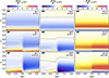 |
Fig. 10. Relaxation rate, ∂F/∂t, in (Jr, cos I) as in Fig. 9, but here from the NR theory (see Appendix H.2 for details). While the in-plane isotropisation and the smoothing of the inclination distribution is recovered, finer details disagree. Here, the amount of relaxation was estimated using finite differentiation using separately regions with positive or negative cos I In effect, this removes the δ′(cos I) singularity in cos I = 0, as discussed in Appendix I. Importantly, the removal of this singularity does not affect the prediction away from cos I = 0. In addition, because this singularity is diluted in N-body measurements – as discussed in Fig. 9 – we do not represent the NR prediction here. |
First, in the absence of rotation, the NR theory predicts a relaxation rate independent of cos I: this is a reassuring sanity check. Yet, when comparing the top rows of Figs. 9 and 10, we note some discrepancies. Namely, the locations of the line of zero relaxation (dashed lines) slightly differ.
The difference is much more striking in the presence of rotation (middle and bottom rows of Fig. 10). In both figures, the orbital reshuffling still operates, and the clusters redistribute their orbits towards smoother distributions of inclinations. Yet, the diffusion structures predicted by the NR theory do not align with the N-body ones. Indeed, N-body simulations (Fig. 9) present “round” structures as one goes from cos I = 0 to cos I = 1. In addition, the relaxation rate decreases as one considers orbits within to rotation plane, that is, as one considers cos I → ± 1. This is in sharp contrast with the “straighter” structures predicted by the NR theory (Fig. 10). Nevertheless, one should keep in mind that Fig. 10 cuts out the singularity at cos I = 0. The comparison to the N-body measurements near cos I = 0 is made difficult by the fact that diffusion at early time is very fast in that region, as shown by Fig. K.4. As a consequence, the measured relaxation rate may suffer from truncation errors – due to, for example, the finite differentiation scheme – the closer one gets to cos I = 0. However, as Fig. K.4 shows, the initial discontinuity appears to have little impact on diffusion both far away from cos I = 0 and beyond t = 0.1 trh. The obtention of a more robust measure would require both a finer time difference and a finer binning of action space. These two improvements would require an ensemble-average over much more realisations to reduce dispersion. A similar conclusion is reached in Appendix J when considering relaxation in (L, cos I).
Before concluding, let us elaborate further on the failure of the NR theory to model out-of-plane relaxation. For α ≠ 0, recall that cos I = ± 1 corresponds to orbits within the rotation plane, while cos I = 0 corresponds to orbits perpendicular to the rotation plane. A test star orbiting in this rotating cluster will torque with all the other stars of the cluster. Equivalently, this means that this star will typically be subject to a torque with the total angular momentum of the rotating cluster, ⟨L⟩ ∝ α ez, the strength of which depends on the test star’s orbital orientation. This is what we observe in Fig. 9. However, the NR theory only takes into account local deflections, and therefore cannot take these coherent interactions into account.
Following the work of Meiron & Kocsis (2019) (see also references therein), we anticipate for VRR to play a key role in these coherent interactions – even after factoring the truncation errors due to the finite difference scheme and the singularity at cos I = 0, both discussed earlier in this section. Indeed, VRR, which is driven by persistent torques between orbital planes, might be needed to explain (i) the faster out-of-plane relaxation (Section 3.3); (ii) the discrepancies between the N-body measurements and the NR predictions. Investigating quantitatively the efficiency of VRR in these systems will be the topic of future investigations.
6. Conclusions and perspectives
6.1. Conclusion
In this paper, we used the NR formalism to probe the long-term time-evolution of rotating anisotropic globular clusters. First, using N-body simulations, we showed how rotation only has a weak impact on the time of core collapse. As such, in contrast with prior research (see, e.g., Hachisu 1979), we did not observe any gravo-gyro catastrophe that could expedite core collapse (see, e.g., Einsel & Spurzem 1999). Since we introduced rotation in a different fashion, this does not contradict previous results.
Focusing on in-plane diffusion, we showed how the NR prediction successfully recovers all the intricacies of the N-body measurements. This is in line with the non-rotating results from T22. Yet, although the diffusion structures in action space closely align, there is still an overall amplitude mismatch between the N-body measurements and the kinetic prediction.
We subsequently turned our interest on out-of-plane relaxation, that is, the redistribution of orbital inclinations. We pointed out the similarities and differences between the N-body measurements and the NR prediction. In both approaches, we observe a systematic reshuffling of orbital inclinations from overpopulated regions to underpopulated ones. As such, the distribution of inclinations get smoother through time, and this process is accelerated by rotation. On the one hand, we observed that the initial discontinuity at cos I = 0 induced a fast relaxation at small times. Surely, this strongly affects any measurement of the relaxation rate in that region. On the other hand, for orbits aligned with the cluster’s rotation plane – where diffusion is much slower and measurements are much easier – the local NR theory does not match with the N-body measurements. We argue that this mismatch originates from the fact that the NR formalism is sourced by local deflections, which neglect the coherent torques between the orbital planes. Accounting for the (efficient) contribution of persistent torques requires the use of VRR.
6.2. Perspectives
Here, the NR formalism was used to describe the very onset of relaxation. Yet, the short duration of our simulations and our limited sample of initial conditions prevented us from fully assessing the asymptotic late time orbital distribution. Naturally, it would be interesting to push the N-body integrations further in time. While some studies carried out such long-term N-body simulations (Tiongco et al. 2020; Livernois et al. 2022), orbital inclinations were, unfortunately, not their focus. Along the same line, it would also be of interest to integrate the 3D FP equation itself. In isotropic clusters, this process has been conducted, as demonstrated for instance in the work of Vasiliev (2015). However, the scenario involving anisotropic, rotating systems has yet to be comprehensively investigated.
Ultimately, if rotation is sufficiently large, it may induce a flattening of the cluster. In that case, Stäckel systems (Dejonghe & de Zeeuw 1988) could be used to model realistic flattened rotating structures. In particular, this would still ensure the integrability of the mean potential, that is the existence of explicit angle-action coordinates. Tailoring secular theory to such setups will be the topic of future works.
In Section 5, we pointed out how the NR theory does not reproduce the out-of-plane diffusion observed in N-body simulations. To understand this mismatch, it would be valuable to examine the predictions of the resonant relaxation (RR) formalism (see, e.g., Hamilton et al. 2018; Fouvry et al. 2021) in the presence of rotation. While the inhomogeneous Landau equation was already investigated in non-rotating isotropic clusters (Hamilton et al. 2018; Fouvry et al. 2021), its implementation in rotating spheres with an explicit dependence on Lz should be the next step. Furthermore, to account for collective effects, an explicit implementation of the Balescu–Lenard equation (Heyvaerts 2010) might prove necessary to match the details of stacked N-body measurements.
Similarly, to get a better handle on the mismatch reported in section 5, one should investigate quantitatively the efficiency of VRR in these clusters (Rauch & Tremaine 1996). This should allow us to determine if indeed coherent and long-lasting torques between orbital planes are the missing ingredients to describe the relaxation of orientations. While this has been extensively studied in galactic nuclei (see, e.g., Eilon et al. 2009; Kocsis & Tremaine 2011, 2015; Szölgyén & Kocsis 2018; Fouvry et al. 2019; Szölgyén et al. 2019, 2021; Magnan et al. 2022), the implementation of VRR in globular clusters should be the topic of future work (see Meiron & Kocsis 2019, for a preliminary investigation).
It would be interesting to leverage multiple masses into the theory, so as to capture (radial or inclination) segregation effects (Meiron & Kocsis 2019). Dekel et al. (2023) argues for instance that the excess of massive galaxies found at very high redshift by the James Webb Space Telescope could originate from early feedback-free star formation within dense, possibly rotating stellar clusters made of massive stars. The fate of such clusters should be captured by the present secular theory. In particular, it could lead to the formation of intermediate mass BHs (Greene & Ho 2004; Greene et al. 2020) and possibly seeds for supermassive BHs (Kormendy & Ho 2013).
Data availability
The data underlying this article is available through reasonable request to the authors. The code, written in JULIA (Bezanson et al. 2017), computing the NR diffusion coefficients in anisotropic rotating clusters is available at the URL: https://github.com/KerwannTEP/CARP.
We will justify the assumption of spherical symmetry in Section 3.1.
Using cos I as an effective coordinate to describe relaxation might be problematic for some clusters. We refer to Appendix K for more details.
For a Plummer cluster, this is related to the Plummer scale length b by the relation Rv = 16b/(3π) (see, e.g., Dejonghe 1987).
Acknowledgments
This work is partially supported by the grant https://www.secular-evolution.org ANR-19-CE31-0017 of the French Agence Nationale de la Recherche, and by the Idex Sorbonne Université. We also thank the KITP for hosting the workshop https://www.cosmicweb23.org during which this project was advanced. This work is partially supported by the National Science Foundation under Grant No. NSF PHY-1748958 and Grant No. AST-2310362. We are grateful to M. Roule, M. Petersen, A. L. Varri and the members of the Segal collaboration for numerous suggestions during the completion of this work. We thank Stéphane Rouberol for the smooth running of the Infinity cluster, where the simulations were performed. Finally, we thank our referee, Prof. Douglas Heggie, for his remarks, which contributed greatly to the improvement of this paper.
References
- Aarseth, S. J., Hénon, M., & Wielen, R. 1974, A&A, 37, 183 [NASA ADS] [Google Scholar]
- Akiyama, K., & Sugimoto, D. 1989, PASJ, 41, 991 [NASA ADS] [Google Scholar]
- Bar-Or, B., & Alexander, T. 2016, ApJ, 820, 129 [NASA ADS] [CrossRef] [Google Scholar]
- Bellini, A., Anderson, J., Bedin, L. R., et al. 2017, ApJ, 842, 6 [NASA ADS] [CrossRef] [Google Scholar]
- Bezanson, J., Edelman, A., Karpinski, S., & Shah, V. B. 2017, SIAM Rev., 59, 65 [Google Scholar]
- Bianchini, P., Varri, A. L., Bertin, G., & Zocchi, A. 2013, ApJ, 772, 67 [NASA ADS] [CrossRef] [Google Scholar]
- Bianchini, P., van der Marel, R. P., del Pino, A., et al. 2018, MNRAS, 481, 2125 [Google Scholar]
- Binney, J., & Tremaine, S. 2008, Galactic Dynamics, 2nd edn. (Princeton Univ Press) [Google Scholar]
- Breen, P. G., Varri, A. L., & Heggie, D. C. 2017, MNRAS, 471, 2778 [NASA ADS] [CrossRef] [Google Scholar]
- Casertano, S., & Hut, P. 1985, ApJ, 298, 80 [Google Scholar]
- Chandrasekhar, S. 1943, ApJ, 97, 255 [Google Scholar]
- Cohn, H. 1979, ApJ, 234, 1036 [NASA ADS] [CrossRef] [Google Scholar]
- Dejonghe, H. 1986, Phys. Rep., 133, 217 [NASA ADS] [CrossRef] [Google Scholar]
- Dejonghe, H. 1987, MNRAS, 224, 13 [NASA ADS] [CrossRef] [Google Scholar]
- Dejonghe, H., & de Zeeuw, T. 1988, ApJ, 333, 90 [NASA ADS] [CrossRef] [Google Scholar]
- Dekel, A., Sarkar, K. C., Birnboim, Y., Mandelker, N., & Li, Z. 2023, MNRAS, 523, 3201 [NASA ADS] [CrossRef] [Google Scholar]
- Eilon, E., Kupi, G., & Alexander, T. 2009, ApJ, 698, 641 [CrossRef] [Google Scholar]
- Einsel, C., & Spurzem, R. 1999, MNRAS, 302, 81 [NASA ADS] [CrossRef] [Google Scholar]
- Ernst, A., Glaschke, P., Fiestas, J., Just, A., & Spurzem, R. 2007, MNRAS, 377, 465 [NASA ADS] [CrossRef] [Google Scholar]
- Fabricius, M. H., Noyola, E., Rukdee, S., et al. 2014, ApJ, 787, L26 [NASA ADS] [CrossRef] [Google Scholar]
- Ferraro, F. R., Mucciarelli, A., Lanzoni, B., et al. 2018, ApJ, 860, 50 [NASA ADS] [CrossRef] [Google Scholar]
- Fiestas, J., & Spurzem, R. 2010, MNRAS, 405, 194 [NASA ADS] [Google Scholar]
- Foote, H. R., Generozov, A., & Madigan, A.-M. 2020, ApJ, 890, 175 [NASA ADS] [CrossRef] [Google Scholar]
- Fouvry, J.-B., Bar-Or, B., & Chavanis, P.-H. 2019, ApJ, 883, 161 [NASA ADS] [CrossRef] [Google Scholar]
- Fouvry, J.-B., Hamilton, C., Rozier, S., & Pichon, C. 2021, MNRAS, 508, 2210 [CrossRef] [Google Scholar]
- Geyer, E. H., Hopp, U., & Nelles, B. 1983, A&A, 125, 359 [Google Scholar]
- Giersz, M., & Heggie, D. C. 1994, MNRAS, 268, 257 [NASA ADS] [CrossRef] [Google Scholar]
- Ginat, Y. B., Panamarev, T., Kocsis, B., & Perets, H. B. 2023, MNRAS, 525, 4202 [Google Scholar]
- Greene, J. E., & Ho, L. C. 2004, ApJ, 610, 722 [NASA ADS] [CrossRef] [Google Scholar]
- Greene, J. E., Strader, J., & Ho, L. C. 2020, ARA&A, 58, 257 [Google Scholar]
- Gruzinov, A., Levin, Y., & Zhu, J. 2020, ApJ, 905, 11 [NASA ADS] [CrossRef] [Google Scholar]
- Hachisu, I. 1979, PASJ, 31, 523 [Google Scholar]
- Hachisu, I. 1982, PASJ, 34, 313 [NASA ADS] [Google Scholar]
- Hamilton, C., Fouvry, J.-B., Binney, J., & Pichon, C. 2018, MNRAS, 481, 2041 [NASA ADS] [CrossRef] [Google Scholar]
- Heggie, D., & Hut, P. 2003, The Gravitational Million-Body Problem (Cambridge University Press) [CrossRef] [Google Scholar]
- Heggie, D. C., & Mathieu, R. D. 1986, in The Use of Supercomputers in Stellar Dynamics, eds. P. Hut, & S. L. W. McMillan (Berlin: Springer), 267, 233 [NASA ADS] [CrossRef] [Google Scholar]
- Heyvaerts, J. 2010, MNRAS, 407, 355 [NASA ADS] [CrossRef] [Google Scholar]
- Inagaki, S., & Hachisu, I. 1978, PASJ, 30, 39 [NASA ADS] [Google Scholar]
- Jindal, A., Webb, J. J., & Bovy, J. 2019, MNRAS, 487, 3693 [Google Scholar]
- Kamann, S., Husser, T.-O., Dreizler, S., et al. 2018, MNRAS, 473, 5591 [NASA ADS] [CrossRef] [Google Scholar]
- Kamlah, A. W. H., Spurzem, R., Berczik, P., et al. 2022, MNRAS, 516, 3266 [CrossRef] [Google Scholar]
- Kim, E., Einsel, C., Lee, H. M., Spurzem, R., & Lee, M. G. 2002, MNRAS, 334, 310 [NASA ADS] [CrossRef] [Google Scholar]
- Kim, E., Lee, H. M., & Spurzem, R. 2004, MNRAS, 351, 220 [NASA ADS] [CrossRef] [Google Scholar]
- King, I. R. 1966, AJ, 71, 64 [Google Scholar]
- Kocsis, B., & Tremaine, S. 2011, MNRAS, 412, 187 [NASA ADS] [CrossRef] [Google Scholar]
- Kocsis, B., & Tremaine, S. 2015, MNRAS, 448, 3265 [NASA ADS] [CrossRef] [Google Scholar]
- Kontizas, E., Kontizas, M., Sedmak, G., & Smareglia, R. 1989, AJ, 98, 590 [Google Scholar]
- Kormendy, J., & Ho, L. C. 2013, ARA&A, 51, 511 [Google Scholar]
- Lagoute, C., & Longaretti, P. Y. 1996, A&A, 308, 441 [NASA ADS] [Google Scholar]
- Lanzoni, B., Ferraro, F. R., Mucciarelli, A., et al. 2018, ApJ, 865, 11 [NASA ADS] [CrossRef] [Google Scholar]
- Livernois, A. R., Vesperini, E., Varri, A. L., Hong, J., & Tiongco, M. 2022, MNRAS, 512, 2584 [NASA ADS] [CrossRef] [Google Scholar]
- Lynden-Bell, D. 1960, MNRAS, 120, 204 [NASA ADS] [Google Scholar]
- Lynden-Bell, D., & Wood, R. 1968, MNRAS, 138, 495 [NASA ADS] [Google Scholar]
- Magnan, N., Fouvry, J.-B., Pichon, C., & Chavanis, P.-H. 2022, MNRAS, 514, 3452 [NASA ADS] [CrossRef] [Google Scholar]
- McLaughlin, D. E., & van der Marel, R. P. 2005, ApJs, 161, 304 [NASA ADS] [CrossRef] [Google Scholar]
- Meiron, Y., & Kocsis, B. 2019, ApJ, 878, 138 [NASA ADS] [CrossRef] [Google Scholar]
- Miocchi, P., Lanzoni, B., Ferraro, F. R., et al. 2013, ApJ, 774, 151 [Google Scholar]
- Rauch, K. P., & Tremaine, S. 1996, New. Astron., 1, 149 [NASA ADS] [CrossRef] [Google Scholar]
- Risken, H. 1996, The Fokker-Planck Equation, 2nd edn. (Berlin: Springer) [CrossRef] [Google Scholar]
- Rosenbluth, M. N., MacDonald, W. M., & Judd, D. L. 1957, Phys. Rev., 107, 1 [NASA ADS] [CrossRef] [Google Scholar]
- Rozier, S., Fouvry, J.-B., Breen, P. G., et al. 2019, MNRAS, 487, 711 [CrossRef] [Google Scholar]
- Sollima, A., Baumgardt, H., & Hilker, M. 2019, MNRAS, 485, 1460 [Google Scholar]
- Spitzer, L. 1975, Dynamics of Stellar Systems, 69, 3 [NASA ADS] [CrossRef] [Google Scholar]
- Stetson, P. B., Pancino, E., Zocchi, A., Sanna, N., & Monelli, M. 2019, MNRAS, 485, 3042 [Google Scholar]
- Szölgyén, Á., & Kocsis, B. 2018, Phys. Rev. Lett., 121, 101101 [CrossRef] [Google Scholar]
- Szölgyén, Á., Meiron, Y., & Kocsis, B. 2019, ApJ, 887, 123 [CrossRef] [Google Scholar]
- Szölgyén, Á., Máthé, G., & Kocsis, B. 2021, ApJ, 919, 140 [CrossRef] [Google Scholar]
- Tep, K., Fouvry, J.-B., & Pichon, C. 2022, MNRAS, 514, 875 [CrossRef] [Google Scholar]
- Tiongco, M., Vesperini, E., & Varri, A. L. 2016, MNRAS, 461, 402 [NASA ADS] [CrossRef] [Google Scholar]
- Tiongco, M., Vesperini, E., & Varri, A. L. 2020, IAU Symp., 351, 524 [NASA ADS] [Google Scholar]
- Tiongco, M., Collier, A., & Varri, A. L. 2021, MNRAS, 506, 4488 [NASA ADS] [CrossRef] [Google Scholar]
- Tiongco, M., Vesperini, E., & Varri, A. L. 2022, MNRAS, 512, 1584 [NASA ADS] [CrossRef] [Google Scholar]
- Trager, S. C., King, I. R., & Djorgovski, S. 1995, AJ, 109, 218 [NASA ADS] [CrossRef] [Google Scholar]
- Varri, A. L., & Bertin, G. 2012, A&A, 540, A94 [NASA ADS] [CrossRef] [EDP Sciences] [Google Scholar]
- Vasiliev, E. 2015, MNRAS, 446, 3150 [NASA ADS] [CrossRef] [Google Scholar]
- Wang, L., Spurzem, R., Aarseth, S., et al. 2015, MNRAS, 450, 4070 [NASA ADS] [CrossRef] [Google Scholar]
- Watkins, L. L., van der Marel, R. P., Bellini, A., & Anderson, J. 2015, ApJ, 803, 29 [Google Scholar]
- White, R. E., & Shawl, S. J. 1987, ApJ, 317, 246 [NASA ADS] [CrossRef] [Google Scholar]
- Wilson, C. P. 1975, AJ, 80, 175 [NASA ADS] [CrossRef] [Google Scholar]
Appendix A: Non-resonant theory
In this Appendix, we detail the derivation of equation (3). This is the backbone of our computation of the NR theory.
A.1. Local velocity coefficients
The starting point are equations (2). We consider this relation within the frame from Fig. A.1. The local velocity deflections are then given by

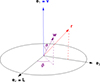 |
Fig. A.1. Tailored frame used to compute the parallel and perpendicular local velocity deflections in equations (A.1). By construction, the test star’s angular momentum L is along the axis e2. |
where the coordinate 1 is the z coordinate, parallel to v. The coordinates 2 and 3 are defined such that the projection of r on the (Oxy) plane is along e3 (Fig. A.1). We now introduce w = v − v′ and change the integration variables from v′ to w in equation (2). We get
with the shortened notation Frot = Frot(r, v′ = v − w). Using these equations allows us to compute the needed coefficients from equation (A.1) through
We now define the spherical coordinates associated with this frame (Fig. A.1)

Injecting equations (A.4) into equations (A.3), we obtain
Here, the background distribution, Frot, is to be evaluated in  . We compute these arguments in appendix A.2. Finally injecting equation (A.5) into equation (A.1), we obtain our main result, namely equation (3), as given in the main text.
A.2. Arguments of the background distribution
Let us now compute the arguments E′, L′ and  for the background distribution function,
  , in equation (2).
We start with E′. It reads

since v = v e1 (see Fig. A.1). This form allows us to get an upper bound on the w-integral of equation (A.5), above which E′ > 0. As soon as E′ > 0, the background star is unbound and its DF vanishes.
The computation of L′ and  is best achieved by using a different coordinate system, as illustrated in Figs. A.1 and A.2. More precisely, the frame (1, 2, 3) is related to the (X, Y, Z) one through the relations
![$$ \begin{aligned} \left[\begin{array}{l} \mathbf e _1\\ \mathbf e _2 \\ \mathbf e _3 \end{array}\right]= \left[ \begin{array}{ccc} \frac{v_{\mathrm{r}}}{v} \cos \varphi - \frac{v_{\mathrm{t}}}{v} \sin \varphi&\frac{v_{\mathrm{r}}}{v}\sin \varphi + \frac{v_{\mathrm{t}}}{v} \cos \varphi&0 \\ 0&0&1 \\ \frac{v_{\mathrm{r}}}{v}\sin \varphi + \frac{v_{\mathrm{t}}}{v} \cos \varphi&\frac{v_{\mathrm{t}}}{v} \sin \varphi - \frac{v_{\mathrm{r}}}{v} \cos \varphi&0 \end{array} \right] \left[\begin{array}{l} \displaystyle \mathbf{e _X }\\ \displaystyle \mathbf{e _Y} \\ \displaystyle { \mathbf e _Z} \end{array}\right], \end{aligned} $$](/articles/aa/full_html/2024/09/aa49465-24/aa49465-24-eq24.gif)
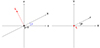 |
Fig. A.2. Illustration of the frames used to compute the argument of the background DF, |

with vr (resp. vt) the radial (resp. tangential) component of the test star’s velocity. We can finally relate the frame (X, Y, Z) to the frame (x, y, z) through the relations
![$$ \begin{aligned} \left[\begin{array}{l} \mathbf e _X \\ \mathbf e _Y\\ \mathbf e _Z \end{array}\right]&= \left[\begin{array}{ccc} \cos I&0&\sin I \\ 0&1&0 \\ -\sin I&0&\cos I \end{array}\right] \left[\begin{array}{l} \displaystyle \mathbf{e _x }\\ \displaystyle \mathbf{e _y} \\ \displaystyle \mathbf{e _z} \end{array}\right]. \end{aligned} $$](/articles/aa/full_html/2024/09/aa49465-24/aa49465-24-eq26.gif)
We can now compute L, the norm of L. As it is a norm, we can choose any frame to compute it. The frame (1, 2, 3) is a convenient choice as this frame is used to compute the integrands of equations (A.3). We write

where (r1, r2, r3) are the coordinates of r in the frame (1, 2, 3). Using equations (A.7) and (A.8), we obtain
Therefore, one gets
given that v′ = v − w.
Let us finally compute  . In the (x, y, z) frame, it reads
From equation (A.8), the positions read


using X = r cos φ and Y = r sin φ. We then obtain the velocities


by taking the time derivative of equations (A.13). Let us now compute the background velocity components. First, using the left panel of Fig. A.2, we have
![$$ \begin{aligned} \left[\begin{array}{l} v^{\prime }_x\\ v^{\prime }_y\\ v^{\prime }_z \end{array}\right]&= \left[\begin{array}{ccc} \cos I&0&-\sin I \\ 0&1&0 \\ \sin I&0&\cos I \end{array}\right] \left[\begin{array}{l} \displaystyle {v^{\prime }_X }\\ \displaystyle {v^{\prime }_Y} \\ \displaystyle {v^{\prime }_Z} \end{array}\right]. \end{aligned} $$](/articles/aa/full_html/2024/09/aa49465-24/aa49465-24-eq38.gif)
Second, using the relation in equations (A.7) (Fig. A.1 and right panel of Fig. A.2), we have
![$$ \begin{aligned} \left[\begin{array}{l} v^{\prime }_X\\ v^{\prime }_Y \\ v^{\prime }_Z \end{array}\right]= \left[ \begin{array}{ccc} \frac{v_{\mathrm{r}}}{v} \cos \varphi - \frac{v_{\mathrm{t}}}{v} \sin \varphi&0&\frac{v_{\mathrm{r}}}{v} \sin \varphi + \frac{v_{\mathrm{t}}}{v}\cos \varphi \\ \frac{v_{\mathrm{r}}}{v} \sin \varphi + \frac{v_{\mathrm{t}}}{v}\cos \varphi&0&\frac{v_{\mathrm{t}}}{v} \sin \varphi - \frac{v_{\mathrm{r}}}{v} \cos \varphi \\ 0&1&0 \end{array}\right] \left[\begin{array}{l} \displaystyle {v^{\prime }_1 }\\ \displaystyle {v^{\prime }_2} \\ \displaystyle {v^{\prime }_3} \end{array}\right]. \end{aligned} $$](/articles/aa/full_html/2024/09/aa49465-24/aa49465-24-eq39.gif)
Overall, we can rewrite equation (A.12) as
Finally, using the Cauchy–Schwarz inequality, one can check that
which ensures that  .
.
Equations (A.6), (A.11) and (A.17) are the main results of this section. They provide us with explicit expressions for the arguments at which to evaluate  in equation (3).
Appendix B: 3D diffusion coefficients
The local in-plane diffusion coefficients, that is, the diffusion coefficients in E and L, are given in appendix C of Bar-Or & Alexander (2016). We reproduce them here for completeness. They read


In order to compute the 3D FP equation (1), we also need the local diffusion coefficients involving Lz = L ⋅ ez. Performing a first-order variation of L = r × v, we can write
where (e1, e2, e3) is the frame illustrated in Fig. A.1. We can then write
As a result, it follows that
with φ given in Fig. (A.2) and vz by equation (A.14c). Overall, we finally have
Equations (B.1) and (B.5) are the main results of this section. They allow us to compute the local diffusion coefficients in (E, L, Lz) from the local velocity diffusion coefficients given by equation (3).
Appendix C: Orbit average
The computation of the global diffusion coefficients in the FP equation (1) requires that we orbit average the local diffusion coefficients over the mean field orbit of the test star. Since the background cluster is rotating, this average involves a radial integration, but also an angular one. This is what we detail here.
C.1. Angular orbit average
We start from the generic formula of equation (4). There, the average with respect to φ must be performed with care since  depends on φ (equation A.17). Fortunately, taking advantage of the particular structure of the diffusion coefficients in E, L and Lz (see equations B.1 and B.5), we only need to compute the following four integrals over φ
where we used  for convenience.
In equation (3), the only dependence with respect to φ is in the dependence with respect to  in Frot. In the particular case of the LBD (equation 5), we can perform explicitly the average over φ. Computing the integrals (C.1) only requires the evaluation of the two non-trivial integrals
with  following from equation (A.17). Introducing
  and
and  , these two integrals can be explicitly computed. Their expressions are gathered in Table C.1. This is the main result of this section.
Explicit values of A1 and A2 (equation C.2a) for the LBD DF (equation 5).
From the numerical point of view, this analytical calculation allows us to speed up the computation of the NR predictions, as the angular integral is removed. In addition, it also explicitly deals with the discontinuity of the LBD DF: this enhances the numerical stability.
C.2. Radial orbit average
Having performed the angle average in Appendix C.1, equation (4) takes the form
where ⟨ ⋅ ⟩φ stands for the angle average. As described in appendix F2 of T22, equation (C.3) can be efficiently performed by changing variable from the radius to an effective anomaly. In particular, this removes the integrable singularity 1/|vr| at pericentre and apocentre. We follow the exact same approach here, and perform the radial average using 50 sampling nodes.
Appendix D: Fokker–Planck and coordinates
Depending on the quantities we wish to investigate, we may wish to change of coordinates system. Fortunately, it is possible to transform one FP description into another under a change of variable. We describe a few relevant examples in this appendix.
D.1. Generic change of coordinates
Given some coordinates x, the FP equation generically reads (Risken 1996)
![$$ \begin{aligned} \frac{{\partial } F({\boldsymbol{x}},t)}{{\partial } t}&= - \frac{{\partial } }{{\partial } {\boldsymbol{x}}} \cdot {\boldsymbol{\mathcal{F} }}_{{\boldsymbol{x}}} ({\boldsymbol{x}})\\&= - \frac{{\partial } }{{\partial } {\boldsymbol{x}}} \cdot \bigg [ {\boldsymbol{D}}_{{\boldsymbol{x}}} ({\boldsymbol{x}}) \, F({\boldsymbol{x}})- \frac{1}{2} \frac{{\partial } }{{\partial } {\boldsymbol{x}}} \!\cdot \! \bigg ( {\boldsymbol{D}}_{{\boldsymbol{x}}{\boldsymbol{x}}} ({\boldsymbol{x}}) \, F({\boldsymbol{x}}) \bigg ) \bigg ] ,\nonumber \end{aligned} $$](/articles/aa/full_html/2024/09/aa49465-24/aa49465-24-eq69.gif)
with the diffusion coefficients
and the DF in x space, F(x). In our case, depending on the context, x = (x1, x2, x3) may either stand for (E, L, Lz), (Jr, L, Lz) or (Jr, L, cos I).
Following Risken (1996) and Bar-Or & Alexander (2016), one can easily rewrite the FP equation within some new coordinates x′(x). The new diffusion coefficients read
These coefficients source a FP equation in x′-space for the DF, F′(x′), reading
with |∂x/∂x′| the inverse Jacobian of the coordinate transform.
D.2. From (E, L, Lz) to (Jr, L, Lz)
Following section 2, we have at our disposal diffusion coefficients within the coordinates (E, L, Lz). Owing to equations (D.3), the diffusion coefficients in the action space (Jr[E, L],L, Lz) are easily computed. This is already detailed in appendix F3 of T22. Ultimately, we have at our disposal the diffusion coefficients
![$$ \begin{aligned} {\boldsymbol{D}}_{1} ({\boldsymbol{J}})\!=\! \left[\begin{array}{l} D_{J_{\mathrm{r}}}\\ D_{L}\\ D_{L_{z}} \end{array}\right] ; \quad {\boldsymbol{D}}_{2} ({\boldsymbol{J}}) \!=\! \left[\begin{array}{ccc} D_{J_{\mathrm{r}}J_{\mathrm{r}}} \!\!\!&\!\!\! D_{J_{\mathrm{r}} L} \!\!\!&\!\!\!D_{J_{\mathrm{r}} L_{z}} \\ D_{J_{\mathrm{r}} L} \!\!\!&\!\!\! D_{L L} \!\!\!&\!\!\!D_{LL_{z}} \\ D_{J_{\mathrm{r}} L_{z}} \!\!\!&\!\!\! D_{LL_{z}} \!\!\!&\!\!\!D_{L_{z}L_{z}} \end{array}\right]\! ,\! \end{aligned} $$](/articles/aa/full_html/2024/09/aa49465-24/aa49465-24-eq74.gif)
which source the FP evolution of Frot(Jr, L, Lz), the cluster’s DF in (Jr, L, Lz).
D.3. From (Jr, L, Lz) to (Jr, L, cos I)
Let us now change of coordinates from J = (Jr, L, Lz) to Jc = (Jr, L, cos I = Lz/L). Applying equations (D.3), we obtain the new diffusion coefficients

while the other coefficients stay unchanged. Importantly, we point out that DJr cos I = DL cos I = 0. This comes from the relations DELz = cos I DEL and DLLz = cos I DLL, which are inferred from equations (B.1) and (B.5). Hence, we are left with the diffusion coefficients
![$$ \begin{aligned} {\boldsymbol{D}}_{1} ({\boldsymbol{J}_{\mathrm{c}}})\!=\! \left[\begin{array}{l} D_{J_{\mathrm{r}}}\\ D_{L}\\ D_{\cos \! I} \end{array}\right] ; \quad {\boldsymbol{D}}_{2} ({\boldsymbol{J}_{\mathrm{c}}}) \!=\! \left[\begin{array}{ccc} D_{J_{\mathrm{r}}J_{\mathrm{r}}} \!\!\!&\!\!\! D_{J_{\mathrm{r}} L} \!\!\!&\!\!\!0 \\ D_{J_{\mathrm{r}} L} \!\!\!&\!\!\! D_{L L} \!\!\!&\!\!\!0 \\ 0 \!\!\!&\!\!\! 0 \!\!\!&\!\!\!D_{\cos \! I\!\cos \! I} \end{array}\right]\! .\! \end{aligned} $$](/articles/aa/full_html/2024/09/aa49465-24/aa49465-24-eq79.gif)
Overall, they drive the FP evolution of F(Jc) = LFrot(J), the cluster’s DF in (Jr, L, cos I).
Appendix E: N-body simulations
The simulations presented throughout the main text were performed using the direct N-body code NBODY6++GPU (Wang et al. 2015), version 4.1. We used the exact same run parameters as in appendix G of T22, and drew the initial conditions using PLUMMERPLUS.PY (Breen et al. 2017). We also refer to the aforementioned appendix for the N-body measurements, and to Table E.1 for all our binning parameters.
Detailed parameters for the measurements in N-body simulations, following the same notation as in appendix G1 of T22. To measure relaxation rate in Fig. 7, we bin the (Jr, L) domain in NJr × NL uniform bins within the region  (similarly for L). We use a similar approach for (Jr, cos I) and (L, cos I). All quantities are in physical units G = M = b = 1, if not stated otherwise.
Each N-body realisation was composed of N = 105 (resp. N = 104) stars and integrated up to tmax = 1000 HU (resp. tmax = 4000 HU) with a dump every 1HU. On a 40-core CPU node with a single V100 GPU, one simulation typically required ∼24 h (resp. ∼12 h) of computation. Ensemble averages were performed over 50 independent runs.
In practice, the main difficulties in the N-body measurements are (i) the estimation of the instantaneous potential – necessary to compute the instantaneous radial action, Jr; (ii) the determination of the bins’ size in action space; (iii) the estimation of the relaxation rate ∂F/∂t via finite differences. This is especially true for highly tangentially anisotropic clusters (e.g., q = − 6), where stars are closely stacked near the Jr = 0 axis. For these three difficulties, we use the same approach as in T22.
Appendix F: Sphericity
In order to track the clusters’ sphericity in Fig. 2, we introduce the 3D inertia-like matrix
with rk the location of the k-th particle, ρk its local density (see Casertano & Hut 1985) and I the 3D identity matrix. In that definition, the extra  factors enhance the contributions from the regions close to the centre.
The matrix ℐ is obviously symmetric. It is also semi-definite positive since for any y ∈ ℝ3, we have
following Cauchy–Schwarz’s inequality. As a result, ℐ has three positive eigenvalues, {λi}i, which encapsulate the cluster’s sphericity. Indeed, spherically symmetric clusters have all their eigenvalues equal.
We generically define the cluster’s sphericity via h = λmin/λmax, which we estimated from N-body simulations. To reduce shot noise in that measurement, we averaged h over realisations as follows. First, we computed the elementary symmetric polynomials α = λ1 + λ2 + λ3, β = λ1λ2 + λ1λ3 + λ2λ3 and γ = λ1λ2λ3 for every cluster and every timestep. We then averaged the values of (α, β, γ) over all realisations. From these values, we estimated the eigenvalues λi as the three (positive) roots of the polynomial λ3 − ⟨α⟩λ2 + ⟨β⟩λ − ⟨γ⟩.4
In Fig. 2, we illustrate the evolution of the sphericity, h, for various amounts of anisotropy and rotation. We typically find h ≃ 0.996, that is, clusters remain reasonably spherically symmetric throughout their evolution. As as visual check of this conclusion, we represent in Fig. F.1 the late time stellar distribution of a rotating isotropic globular cluster with N = 104. Even close to core collapse, the cluster remains spherically symmetric.
 |
Fig. F.1. Snapshots of the distribution of stars in a rotating (α = 0.25) isotropic (q = 0) Plummer cluster with N = 104 stars, projected on the rotation plane. From left to right, this corresponds to t = 0, 1000, 2000, 3000 HU. As time evolves, the cluster contracts and the central density increases. Notwithstanding, the cluster retains its initial spherical symmetry. |
Appendix G: Rotating King model
In section 3.2, we mentioned the gravo-gyro catastrophe, introduced in Hachisu (1979) as the rotational counterpart of the gravothermal catastrophe (Lynden-Bell & Wood 1968) to explain an apparent acceleration of core collapse with rotation. To study this phenomenon, Einsel & Spurzem (1999) considered the secular evolution of a rotating King model with the initial DF

where Frot = Frot(r, v) = Frot(E, Lz) is the DF in (r, v). In this DF,  is an inverse temperature with σc the central velocity dispersion, while
  is a rotation parameter with nc the central density and Ω0 the angular velocity in the cluster’s centre (Lagoute & Longaretti 1996). In particular, β is related to the so-called King parameter (King 1966), defined by W0 = − β(ψ − ψt) where ψt is the potential at the cluster’s edge. The rotating King models from Einsel & Spurzem (1999) can therefore be parametrised by (W0, ω0). In practice, Einsel & Spurzem (1999) integrated these models up to core collapse using a FP scheme in (E, Lz) for different rotation parameters, ω0. This is presented in their fig. 2. In particular, they demonstrated a clear correlation between the time of core collapse and the rotation parameter of the King model. The faster a cluster rotates, the shorter the core collapse time. Importantly, as emphasised in section 3.2, we recall that as one varies ω0, the cluster’s mean potential also varies.
Appendix H: 2D Fokker-Planck equations
In practice, it is convenient to study long-term relaxation through two-dimensional projections of action space. To do so, we must integrate over one coordinate the 3D FP equation expressed either in (Jr, L, Lz) (appendix D.2) or in (Jr, L, cos I) (appendix D.3). In this appendix, we compute the 2D FP equations in (Jr, L), (Jr, cos I) and (L, cos I) that respectively drive the evolution of the DFs
H.1. Equation in (Jr, L)
We start from equation (1), which describes diffusion in (Jr, L, Lz), and write the flux divergence as
Integrating over Lz yields

In addition, because the flux cannot exit action space, we also have ℱLz(Lz = ± L) = ± ℱL(Lz = ± L). As a result, all the non-integral terms in equations (H.3) cancel one another. We are then left with the 2D equation
It is this rewriting that is used in section 4.2. To obtain Fig. 8, the Lz-integrals in equations (H.3) are sampled with 50 nodes. The (w, ϑ, ϕ)-integrals of equations (3) are sampled with 100 w-nodes, 100 ϑ-nodes and 200 ϕ-nodes.
H.2. Equation in (Jr, cos I)
We start from the diffusion coefficients in equation (D.7), which describe diffusion in (Jr, L, cos I), for the DF, F = LFrot. We write the flux divergence as
Integrating over L yields
Because the flux cannot leave action space, equation (H.6b) vanishes. Then, equation (H.5) readily reduces to a 2D FP equation in (Jr, cos I), which we use in section 5.2. To obtain Fig. 10, the L-integrals in equations (H.6) are sampled with 50 nodes for 0 ≤ L ≤ 3 L0, where  is the typical action. The (w, ϑ, ϕ)-integrals of equations (3) are sampled with 100 w-nodes, 100 ϑ-nodes and 800 ϕ-nodes.
H.3. Equation in (L, cos I)
As in appendix H.2, we start from the diffusion coefficients in equation (D.7). Integrating equation (H.5) over Jr yields
Once again, because the flux cannot leave action space, equation (H.7a) vanishes. Then, equation (H.5) reduces to a 2D FP equation in (L, cos I), which we use in appendix J. To obtain Fig. J.2, the Jr-integrals in equations (H.7) are sampled with 50 nodes for 0 ≤ Jr ≤ 10 L0. The (w, ϑ, ϕ)-integrals of equations (3) are sampled with 100 w-nodes, 100 ϑ-nodes and 1600 ϕ-nodes.
Appendix I: Evaluating the discontinuity at cos I = 0
In this appendix, we highlight the sharp discontinuity of the relaxation rate that occurs at cos I = 0 as a result of the discontinuous LBD distribution of orientations (equation 5). This singularity has been removed from Figures 10 and J.2 (see appendices H.2 and H.3). Because equation (5) is discontinuous, we expect that taking the first and second derivatives with respect to cos I will yield a theoretical δ′(cos I) behaviour around cos I = 0. To that aim, we show in Figure I.1 the quantities DcosIFrot and DcosIcosIFrot, respectively with their first and second derivatives with respect to cos I. In particular, ∂2(DcosIcosIFrot)/∂cosI2 has a δ′(cos I) component near cosI = 0. In practice, this is smoothed by the finite differentiation used here. Indeed, reducing the finite differentiation step sharpens the discontinuity to higher and higher values, hence converging to the true δ′(cos I) behaviour.
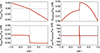 |
Fig. I.1. Representation for a Plummer cluster (q, α) = (0, 0.25) of the cos I terms, DcosIFrot (on the top left) and DcosIcosIFrot (on the top right), respectively with the first (on the bottom left) and second (on the bottom right) derivative with respect to cos I. In particular, the bottom right panel displays an approximate δ′(cos I) behaviour – the amplitude of the jumps tends to infinity as one reduces the step in the finite differentiation scheme – which is the expected theoretical relaxation induced by the sgn discontinuity of Frot at t = 0. |
Appendix J: Relaxation in (L, cos I)
In this appendix, we follow the same approach as in section 5, and investigate relaxation in (L, cos I). We refer to Appendix H.3 for the derivation of the relevant 2D FP equation. In Fig. J.1, we illustrate the N-body measurements while Fig. J.2 presents the associated NR predictions.
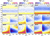 |
Fig. J.1. Same as in Fig. 9 but in (L, cos I). Diffusion reshuffles orbital inclinations toward a more affine distribution in cos I. |
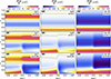 |
Fig. J.2. Same as Fig. 10 but in (L, cos I). The NR prediction fails to recover in detail the diffusion structures observed numerically in Fig. J.1. |
From these two figures, we can globally make the same observations as in section 5, which considered diffusion in (Jr, cos I). Indeed, in rotating clusters, diffusion reshuffles orbits towards smoother distributions of inclinations. Nevertheless, the NR prediction fails at predicting the exact structures measured in N-body simulations. In particular, the NR theory predicts a relaxation rate varying weakly with cos I (for a given sign of cos I). This differs from the N-body simulations, where the relaxation rate decreases away from cos I = 0.
Appendix K: Impact of discontinuities
In this appendix, we investigate in more detail the impact of the discontinuity at cos I = 0, introduced by the LBD (equation 5). To do so, we follow the same approach as in section 2.3 of Rozier et al. (2019) and consider rotating DFs of the form
![$$ \begin{aligned} F_{\mathrm{rot}}(J_{\mathrm{r}},L,L_{z}) = F_{\mathrm{tot}}(J_{\mathrm{r}},L) (1+\alpha g[L_{z}/L]), \end{aligned} $$](/articles/aa/full_html/2024/09/aa49465-24/aa49465-24-eq108.gif)
where g[cos I] is an odd function with g(1) = 1. The LBD corresponds to g = sgn. To approximate smoothly the LBD, we consider the sequence of functions

As illustrated in Fig. K.1, this ensures that g0(x) = x and g∞(x) = sgn(x).
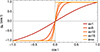 |
Fig. K.1. Family of functions ga(cos I) (equation K.2) for various a. For a → 0, the function approaches identity, while for a → ∞, it approaches the sign function. Varying a allows us to investigate the impact of the LBD discontinuity in equation (5). |
K.1. The cos I coordinate
To probe the possible presence of discontinuities and singularities, let us first compute the cos I component of the 3D flux in (Jr, L, cos I), as introduced in appendix D.3. The dependence of this flux with respect to a is illustrated in Fig. K.2.
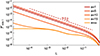 |
Fig. K.2. Diffusion flux along cos I of the 3D FP equation in (Jr, L, cos I), for Jr = 0.1 and cos I = 0.2, as a function of L and for various smooth functions ga (equation K.2). Here, we consider an isotropic cluster with rotation parameter α = 0.25. For any smooth ga, the flux diverges like 1/L for L → 0. As a → ∞, that is, as ga tends to the sgn function, the flux converges to the LBD flux pointwise, which exhibits no divergence. |
In this figure, for any smooth ga, we observe a 1/L divergence of the flux as L → 0. In a nutshell, when working with cos I, we suffer from a coordinate singularity, and the NR prediction cannot be applied to a DF with a smooth rotation function. Yet, when a → ∞, the flux converges towards the LBD flux pointwise, and this flux does not diverge for L → 0. Phrased differently, in the particular case of the LBD sign function, we can make a meaningful and well-posed NR prediction for the diffusion in cos I. In practice, this vanishing of the divergence stems from the cancellation of the derivative of sgn(cos I) everywhere (except for cos I = 0). Such a property is not the norm for smooth arbitrary rotation functions, g(cos I). In that case, the 1/L2 singularities visible in equations (D.6) do not combine into an integrable quantity.
To further stress that this divergence originate from coordinate singularities, let us now produce NR predictions by describing relaxation in (Jr, L, Lz) rather than in (Jr, L, cos I). To do so, we define the DF in Lz as
Integrating the 3D FP equation (1) over Jr and L yields
![$$ \begin{aligned} \frac{{\partial } F (L_{z})}{{\partial } t} = -\frac{{\partial } }{{\partial } L_{z}}\big (\overline{D}_{L_{z}} F[L_{z}]\big ) + \frac{1}{2} \frac{{\partial }^2}{{\partial } L_{z}^2}\big ( \overline{D}_{L_{z}L_{z}} F[L_{z}]\big ) . \end{aligned} $$](/articles/aa/full_html/2024/09/aa49465-24/aa49465-24-eq111.gif)
Here, the 1D diffusion coefficients in Lz are given by
with Frot(Jr, L | Lz) = Frot(Jr, L, Lz)/F(Lz) standing for the DF in (Jr, L) given Lz, and normalised to unity. Importantly, for Lz ≠ 0, the coefficients  and
and  are well defined whatever the considered rotating DF. In addition, they both converge to some finite values as Lz → 0, as illustrated in Fig. K.3. The absence of any divergence here emphasizes that the divergence observed in Fig. K.2 stems from a coordinate singularity associated with cos I.
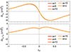 |
Fig. K.3. One-dimensional diffusion coefficients |


K.2. Impact on N-body measurements
To estimate the impact of the discontinuity on relaxation, we used N-body simulations in Fig. K.4 to compare the early relaxation of the discontinuous LBD distribution (equation 5) with its smooth approximation (equation K.2 with a = 10). Reassuringly, we observe a fast dilution of the discontinuity, with the DF quickly resembling its smooth approximation. Afterwards, no significant difference is observed between the two systems.
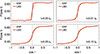 |
Fig. K.4. Comparison between two rotating, isotropic Plummer clusters with parameters (q, α) = (0, 0.25) and N = 105 stars. The discontinuous cluster follows the LBD parametrization (equation 6), while the smooth cluster follow an erf approximation, as defined in eq. (K.2). Both measurements have been ensemble-averaged over 10 realizations. Beyond the initial dilution of the discontinuity, we observe that the initially discontinuous DF joins the smooth DF, after which both systems appear to follow the same evolution. |
All Tables
Detailed parameters for the measurements in N-body simulations, following the same notation as in appendix G1 of T22. To measure relaxation rate in Fig. 7, we bin the (Jr, L) domain in NJr × NL uniform bins within the region (similarly for L). We use a similar approach for (Jr, cos I) and (L, cos I). All quantities are in physical units G = M = b = 1, if not stated otherwise.
All Figures
|
Fig. 1. Illustration of the orbit average in physical space. The test star (in black, part of whose orbit is shown in red) is averaged over all its available positions in its orbital plane, within the radial range of the orbit (r ∈ [rp, ra]) and its angular range (φ ∈ [0, 2π]), weighted by the surface density Ωr/(2π2|vr|). Here, the frame is that of the right panel of Fig. A.2. |
| In the text | |
|
Fig. 2. Sphericity, h, of a sample of rotating anisotropic clusters, as defined in Appendix F, from N-body simulations for N = 105. Each case has been averaged over 50 realisations. We represent radially anisotropic clusters (q = 1) in red, isotropic clusters (q = 0) in yellow, and tangentially anisotropic ones (q = − 6) in blue. For each anisotropy, we consider three rotating parameters α = 0.1, 0.25, 0.5 (ordered from dark to light colors). In agreement with Rozier et al. (2019), some of these clusters are unstable – namely (q, α) = (1, 0.5), and in a smaller fashion (q, α) = (1, 0.25) – while the others are linearly stable and remain spherically symmetric. |
| In the text | |
|
Fig. 3. Core radius as a function of time, as measured in N-body simulations, with trh defined in equation (7). Each case has been averaged over 50 realisations with N = 104. Increasing the rotation strength α slightly reduces the time of core collapse. Nevertheless, the impact of rotation (i.e. the gravo-gyro catastrophe) is surely not as pronounced as what was observed in, e.g., Einsel & Spurzem (1999). |
| In the text | |
|
Fig. 4. Evolution of the angular momentum DF, F(L), as measured in N-body simulations with N = 104, with trh defined in Equation (7). For each parameter, the latest time is close to the time of core collapse. Each panel is averaged over 50 realisations. Here, F(L) redistributes towards lower angular momenta, with details depending on the initial velocity anisotropy. Rotation does not impact strongly the in-plane relaxation. |
| In the text | |
|
Fig. 5. Same as Fig. 4 but for the DF in orbital inclinations, F(cos I). The out-of-plane relaxation does not depend much on the initial velocity anisotropy. As time evolves, the discontinuity of the LBD (Equation (5)) at cos I = 0 is (rapidly) washed out. |
| In the text | |
|
Fig. 6. Initial evolution of the core radius in clusters with N = 105 stars, as measured in N-body simulations. We use that same convention as in Fig. 2. Interestingly, in these stable clusters, rotation only weakly affects the core contraction. |
| In the text | |
|
Fig. 7. Relaxation rate, ∂F/∂t, in (Jr, L) for various velocity anisotropies q (left to right) and rotation parameters α (top and bottom), as measured in N-body simulations. The overall amplitude of the in-plane relaxation rate depends on q, but only very weakly on α. |
| In the text | |
|
Fig. 8. Relaxation rate, ∂F/∂t, in (Jr, L) as in Fig. 7, but here from the NR theory. The prediction matches the N-body measurements from Fig. 7, up to an overall prefactor that depends on q, and (very) weakly on α. |
| In the text | |
|
Fig. 9. Relaxation rate, ∂F/∂t, in (Jr, cos I) for various anisotropies q (left to right) and rotation α (from top to bottom), as measured in N-body simulations. The amplitudes and structures observed depend on anisotropy, and show a reshuffling towards isotropisation. Orientations redistribute toward a more affine distribution in cos I. As a result of using binning in action space and finite difference in time to compute ∂F/∂t, the expected initially sharp relaxation occurring at cos I = 0 has been smoothed and is not visible. |
| In the text | |
|
Fig. 10. Relaxation rate, ∂F/∂t, in (Jr, cos I) as in Fig. 9, but here from the NR theory (see Appendix H.2 for details). While the in-plane isotropisation and the smoothing of the inclination distribution is recovered, finer details disagree. Here, the amount of relaxation was estimated using finite differentiation using separately regions with positive or negative cos I In effect, this removes the δ′(cos I) singularity in cos I = 0, as discussed in Appendix I. Importantly, the removal of this singularity does not affect the prediction away from cos I = 0. In addition, because this singularity is diluted in N-body measurements – as discussed in Fig. 9 – we do not represent the NR prediction here. |
| In the text | |
|
Fig. A.1. Tailored frame used to compute the parallel and perpendicular local velocity deflections in equations (A.1). By construction, the test star’s angular momentum L is along the axis e2. |
| In the text | |
|
Fig. A.2. Illustration of the frames used to compute the argument of the background DF, |
| In the text | |
|
Fig. F.1. Snapshots of the distribution of stars in a rotating (α = 0.25) isotropic (q = 0) Plummer cluster with N = 104 stars, projected on the rotation plane. From left to right, this corresponds to t = 0, 1000, 2000, 3000 HU. As time evolves, the cluster contracts and the central density increases. Notwithstanding, the cluster retains its initial spherical symmetry. |
| In the text | |
|
Fig. I.1. Representation for a Plummer cluster (q, α) = (0, 0.25) of the cos I terms, DcosIFrot (on the top left) and DcosIcosIFrot (on the top right), respectively with the first (on the bottom left) and second (on the bottom right) derivative with respect to cos I. In particular, the bottom right panel displays an approximate δ′(cos I) behaviour – the amplitude of the jumps tends to infinity as one reduces the step in the finite differentiation scheme – which is the expected theoretical relaxation induced by the sgn discontinuity of Frot at t = 0. |
| In the text | |
|
Fig. J.1. Same as in Fig. 9 but in (L, cos I). Diffusion reshuffles orbital inclinations toward a more affine distribution in cos I. |
| In the text | |
|
Fig. J.2. Same as Fig. 10 but in (L, cos I). The NR prediction fails to recover in detail the diffusion structures observed numerically in Fig. J.1. |
| In the text | |
|
Fig. K.1. Family of functions ga(cos I) (equation K.2) for various a. For a → 0, the function approaches identity, while for a → ∞, it approaches the sign function. Varying a allows us to investigate the impact of the LBD discontinuity in equation (5). |
| In the text | |
|
Fig. K.2. Diffusion flux along cos I of the 3D FP equation in (Jr, L, cos I), for Jr = 0.1 and cos I = 0.2, as a function of L and for various smooth functions ga (equation K.2). Here, we consider an isotropic cluster with rotation parameter α = 0.25. For any smooth ga, the flux diverges like 1/L for L → 0. As a → ∞, that is, as ga tends to the sgn function, the flux converges to the LBD flux pointwise, which exhibits no divergence. |
| In the text | |
|
Fig. K.3. One-dimensional diffusion coefficients |
| In the text | |
|
Fig. K.4. Comparison between two rotating, isotropic Plummer clusters with parameters (q, α) = (0, 0.25) and N = 105 stars. The discontinuous cluster follows the LBD parametrization (equation 6), while the smooth cluster follow an erf approximation, as defined in eq. (K.2). Both measurements have been ensemble-averaged over 10 realizations. Beyond the initial dilution of the discontinuity, we observe that the initially discontinuous DF joins the smooth DF, after which both systems appear to follow the same evolution. |
| In the text | |
Current usage metrics show cumulative count of Article Views (full-text article views including HTML views, PDF and ePub downloads, according to the available data) and Abstracts Views on Vision4Press platform.
Data correspond to usage on the plateform after 2015. The current usage metrics is available 48-96 hours after online publication and is updated daily on week days.
Initial download of the metrics may take a while.