| Issue |
A&A
Volume 689, September 2024
|
|
|---|---|---|
| Article Number | A72 | |
| Number of page(s) | 17 | |
| Section | The Sun and the Heliosphere | |
| DOI | https://doi.org/10.1051/0004-6361/202347824 | |
| Published online | 03 September 2024 | |
Investigating and comparing the IRIS spectral lines Mg II, Si IV, and C II for flare precursor diagnostics
1
Astronomical Institute of the University of Bern, Sidlerstrasse 5, 3012 Bern, Switzerland
2
University of Geneva, 7, Route de Drize, 1227 Carouge, Switzerland
Received:
29
August
2023
Accepted:
30
May
2024
Abstract
Context. Reliably predicting solar flares can mitigate the risks of technological damage and enhance scientific output by providing reliable pointings for observational campaigns. Flare precursors in the spectral line Mg II have been identified.
Aims. We extend previous studies by examining the presence of flare precursors in additional spectral lines, such as Si IV and C II, over longer time windows, and for more observations.
Methods. We trained neural networks and XGBoost decision trees to distinguish spectra observed from active regions that lead to a flare and those that did not. To enhance the information within each observation, we tested different masking methods to preprocess the data.
Results. We find average classification true skill statistics (TSS) scores of 0.53 for Mg II, 0.44 for Si IV, and 0.42 for C II. We speculate that Mg II h&k performs best because it samples the highest formation height range, and is sensitive to heating and density changes in the mid- to upper chromosphere. The flaring area relative to the field of view has a large effect on the model classification score and needs to be accounted for. Combining spectral lines has proven difficult, due to the difference in areas of high probability for an imminent flare between different lines.
Conclusions. Our models extract information from all three lines, independent of observational bias or GOES X-ray flux precursors, implying that the physics encoded in a combination of high resolution spectral data could be useful for flare forecasting.
Key words: methods: data analysis / techniques: spectroscopic / Sun: chromosphere / Sun: flares / Sun: transition region
Corresponding author; This email address is being protected from spambots. You need JavaScript enabled to view it. .
© The Authors 2024
 Open Access article, published by EDP Sciences, under the terms of the Creative Commons Attribution License (https://creativecommons.org/licenses/by/4.0), which permits unrestricted use, distribution, and reproduction in any medium, provided the original work is properly cited.
This article is published in open access under the Subscribe to Open model. This email address is being protected from spambots. You need JavaScript enabled to view it. to support open access publication.
1. Introduction
Solar flares can eject billions of tons of solar plasma into space and towards Earth. Charged particles reaching the Earth’s magnetosphere can cause damage to satellite electronics, disrupt air traffic communication and navigation, and in the worst case induce currents in our electrical grid leading to large-scale power outages. Despite the recent progress in our understanding of the solar magnetic field, we still do not completely understand all the physical mechanisms driving solar flares (e.g. Judge et al. 2021). In particular, we do not know if and when an active region will produce a flare or how strong it may be.
Early investigations to find physical features that distinguish flaring from non-flaring active regions focussed on using photospheric magnetic field data, or parameters derived therewith (e.g. Leka & Barnes 2003, 2007). A large-scale study investigating 2071 active regions was carried out by Bobra & Couvidat (2015) who found that only four out of 25 features derived from the photospheric vector magnetic field observed with the Helioseismic Magnetic Imager (HMI, Schou et al. 2012) on board the Solar Dynamics Observatory (SDO, Pesnell et al. 2012) were necessary to reach the highest forecasting scores for flare prediction. But a fully reliable forecast could not be achieved with photospheric data alone, also not in subsequent studies using more and more complex machine-learning techniques (e.g. Florios et al. 2018; Huang et al. 2018; Georgoulis et al. 2021; Deshmukh et al. 2023). It is therefore possible that information extracted from the photospheric magnetic field alone is not sufficient for the complex task of flare prediction and therefore, additional data were considered in further studies.
Nishizuka et al. (2017) included data from the Atmospheric Imaging Assembly (AIA, Lemen et al. 2012) 1600 Å channel, the flare history of each active region, and the full disk-integrated GOES X-ray flux, reaching a true skill statistics (TSS) ∼0.9 for ≥M-class flares. The TSS takes values between minus one and one, where a score of one means perfect prediction, while a score of zero means random guessing and a score of minus one means the model makes completely adverse predictions. They found the flaring history, as well as the area of chromospheric UV brightenings in the AIA 1600 Å channel to be among the strongest indicators for future flares. In a follow-up study, Nishizuka et al. (2018) extended their feature set to include coronal hot brightening events (T ≥ 107 K), and included GOES X-ray flux and AIA 131 Å data one and two hours before the prediction window. They investigated the feasibility of using a deep neural network in an operational manner and split the data into a training set from 2010 until 2014 and testing set on data only from 2015. They reached a slightly lower TSS = 0.80 for ≥M-class flares and TSS = 0.63 for ≥C-class flares than what they reported previously. However, they stated that the results were better than what could be achieved with the previous models in an operational setup. Thus adding those additional features improved the skill scores.
To test whether additional features improve potential flare predictions, Jonas et al. (2018) performed an extensive study on the combination of images from the AIA channels 1600 Å, 171 Å, and 193 Å together with HMI data and active region flare history. However, they did not find any substantial improvement in performance compared to what was previously reported in the literature. Leka et al. (2023) reached similar scores with a non-parametric discriminant analysis (NPDA) as those reported by Jonas et al. (2018) or Nishizuka et al. (2018). Especially features covering short-lived small-scale brightenings scored best in the NPDA for flare prediction. The information covered by HMI and AIA might be limited for solar flare prediction and therefore several studies turned their attention to spectra. NASA’s Interface Region Imaging Spectrograph (IRIS) small explorer spacecraft (De Pontieu et al. 2014) observes spectral lines forming in the chromosphere and transition region, thereby offering insight into the thermodynamic state of those atmospheric layers.
Panos et al. (2018) performed a study on spectra from solar flares observed with IRIS, and found similarities between the spectra of 33 flares in Mg II k, indicating a common flare mechanism. Therefore, a machine-learning approach could potentially identify similarities in active regions before the occurrence of a flare. Panos & Kleint (2020) showed that single spectra in Mg II k from flaring and non-flaring active regions could be separated, using fully connected deep neural networks. The classification was performed on ten precomputed features from the spectra in a time window of 25 minutes before the onset of a flare with only X- and M-class flares allowed in the positive class. For one flare, which they analysed in detail, Panos & Kleint (2020) showed that the classification score was increasing towards the flare, both in time and space.
Woods et al. (2021) clustered Mg II h&k spectra occurring before flares and non-flaring active regions with k-means and showed that Mg II UV triplet emission frequently occurs before flares, and might stem from heating events in the chromosphere, up to 40 minutes before flare onset. The importance of the triplet emission as a precursory feature was independently verified using explainable AI techniques (Panos et al. 2023). Even before the predictive potential of Mg II h&k was realised, Cheng et al. (1984) had found small brightenings occurring in Si IV 30 to 60 minutes before flare onset, and Harra et al. (2001) found hints of turbulent changes in the active region, which started 11 minutes before the hard-X ray signal onset of a flare.
One criticism that remains for studies based on spectra is the rather small sample of observations and time windows investigated. Therefore, for this study we extended the dataset by including many more observations, and extending the time window analysed from 25 minutes to one hour where possible. Reproducing and improving previous results to a broader dataset strengthens the argument for the utility of flare precursor signals to understand the processes leading up to flare onset. Furthermore, we included other spectral lines in addition to Mg II h&k to sample more atmospheric height ranges, and probed the use of spectra from the most dominant spectral lines in the chromosphere and transition region observed by IRIS: Mg II h&k, Si IV, C II, and combinations thereof. In contrast to previous parameterised and single line approaches (Panos & Kleint 2020), we built machine-learning-based classification models using the raw spectra from single spectral lines, and their combinations.
The paper is organised into the following sections: In Section 2, we describe the preparation of the data and introduce the machine-learning methods used for this study, as well as the strategy to estimate the true performance of our models on unseen data. In Section 3, we present the results of the different models cross validated and tested on unseen data. In Section 4, we discuss the capability of our models to classify spectra within that particular observation in terms of meta information (slit position, strength of flare, GOES X-ray flux, etc.). In Section 5 we summarise our results and present the conclusions we draw from this study.
2. Data preparation and classification methods
2.1. Selection of observations
For this study, we used observations of flaring and non-flaring active regions recorded with IRIS. We investigated if there are systematic differences between the spectra observed during the pre-flare phase, which includes all spectra recorded up to the start of the flare, and spectra from observations of active regions which did not lead to a flare. We defined the pre-flare (PF) phase spectra as the positive class and the non-flaring active region (AR) spectra as our negative class. By using classification algorithms to distinguish both classes (PF and AR) we can search for the differences between the two types of spectra, even though we expect an overlap between both classes. This is because we classify the spectra independently from each other and we do not expect that a PF observation is completely free of spectra that could also be found in AR observations. Additionally, in each observation, the rather long spectrograph slit might cover areas that are more similar to the quiet Sun than to the active region. Therefore, we defined another class of spectra, labelled quiet Sun spectra (QS), which represents any spectrum that appears in quiet Sun observations. Once we know the shape of quiet Sun spectra, we are able to remove them from our PF and AR dataset to reduce the number of redundant quiet Sun spectra in our dataset for classification. The procedure to achieve this for the different spectral lines is explained in Sect. 2.3.
The observations and their observational parameters are published on https://zenodo.org/records/115514901 and a small selection is shown in Fig. 1. In particular, we analysed the Mg II h&k lines, without a prior feature selection, and additionally tested the potential for PF and AR classification with Si IV 1403 Å and the C II multiplet around 1335 Å. We also analysed the Si IV 1394 Å, as well as the O I 1356 Å lines, however, for Si IV 1394 Å the results did not differ to those of Si IV 1403 and for O I 1356, the signal to noise was too low for a good convergence of the models. In total we have 74 PF samples from 52 PF observations (meaning several flares in some observations) and 59 samples of ∼one hour long segments from in total 30 AR observations from 2014 until 2022, with various observing modes. We included 16 PF observations of Panos & Kleint (2020) in our study, plus 36 additional PF observations by allowing any flare registered in the Heliophysics Events Knowledgebase (HEK; Hurlburt et al. 2010) corresponding to a flare class greater than ∼C5 in our sample. The flare classes in the HEK database are determined from the original GOES X-ray flux, and we left them unchanged for consistency to other publications. For the AR observations, we included the 18 observations used in other studies (e.g. Panos & Kleint 2020), plus 12 additional observations.
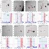 |
Fig. 1. Examples of observations of active regions with IRIS in the continuum channel of HMI, the recalibrated GOES X-ray flux for the time period of the observation, and the flare class from the HEK database. The red frame with the vertical lines displays the FOV and the slit positions of the IRIS spectrograph. In the GOES X-ray flux we show the time window of the IRIS observation as a light blue shaded region. The red shaded region with the vertical line depicts the time of a flare, from beginning to end, according to the HEK database. The black dashed vertical and horizontal line depict the parts that were cut from the observations and used for training and testing the classification models. |
The PF observations were selected according to the following criteria: Flare is not on or over the limb and the slit covers at least part of the flare. This was ensured by looking at the slit-jaw image movies from IRIS for every flare. We selected IRIS observations that start at least 25 minutes before flare onset according to the HEK flare start times and where observations were available, we extended the analysed pre-flare phase to up to one hour before flare onset, and clipped the IRIS observations in time accordingly. The flare start time used from HEK is determined from the GOES soft X-ray flux. We did not make any constraints to the observing mode.
We separated the PF samples into two groups that we labelled blue and yellow. Group blue contains flares that have a flat GOES curve before flare onset for at least one hour and do not show any pre-flare activity in form of small peaks or increasing X-ray flux during that one hour. These groups serve to investigate whether there are observable flare precursors in the lower to mid solar atmosphere not associated with X-ray activity. However, there may still be low X-ray activity hidden within the rest of the integrated X-ray flux from the whole solar disk, showing a flat GOES curve before flare onset nonetheless. Group yellow contains all flares with a non-flat GOES curve but no previous flares within the time range selected as pre-flaring. Our hypothesis is that the PF and AR observations are separable exclusively by learning properties about the spectral shape of individual spectra. Furthermore, if they are separable, we want to test whether there are differences in these flare precursors between spectral lines with different formation height ranges.
2.2. Data preprocessing for model training and validation
We used IRIS level 2 data, and additionally processed the data as follows. We divided all spectra by their exposure time to get the intensity per wavelength in DN/s. Then we filtered all spectra for cosmic rays with a Laplacian edge detection algorithm (van Dokkum 2001) applied to the level 2 raster cubes. The method is provided by the astroscrappy (McCully et al. 2018) python library under detect_cosmics. We removed any spectrum containing cosmic rays from our dataset. A visual inspection of spectra after filtering from cosmic rays showed that most spectra containing cosmic rays could be removed. An example of spectrograms with the position of the slit on the slit-jaw image is shown in Fig. 2.
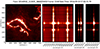 |
Fig. 2. Example of IRIS spectra used for this study, showing the three considered spectral lines Mg II, C II, and Si IV. The IRIS spectrograph slit is visible as a vertical black line in the flare image at location x ∼ 370. |
We also rejected any overexposed spectrum (in at least three wavelength points) or spectra with missing data (at least one value below −100), and finally applied a minimum threshold in DN/s criterion to reject any spectra not reaching a sufficient signal-to-noise ratio. The threshold was selected for each line individually by investigating the spectra by eye and comparing slit-jaw images while masking out the rejected pixels. The number of spectra removed in the individual steps for each line are presented in Table 1.
Number of spectra removed in each preprocessing step.
Additionally, for Mg II h&k we applied the following extra steps: We excluded spectra (1) if their maximum value occurred spectrally far from the line core (outside of 2794.85 to 2797.85 Å for the k-line and 2802.02 to 2805.02 Å for the h-line), (2) with high continuum (mean intensity between 2799.75 and 2800.24 Å ≥0.6 times the maximum intensity), or (3) where the k/h ratio (integrated over the line core windows) was outside of [0.8, 2], for which theoretical bounds predict a ratio between [1, 2] (see e.g. Panos et al. 2018; Kastner 1993 for a detailed explanation).
We linearly interpolated the spectra onto a common wavelength grid for each line. The parameters used for the grid are presented in Table 2. To verify our procedure to remove certain spectra from our dataset, we created histogram plots of spectral features, similar to those used in Panos & Kleint (2020) to ensure that our data follow a Gaussian distribution. We did so as well for the coordinates of each observation, the cadence and the observation types, to make sure our set is not biassed in general or between the different classes (PF, AR, QS). The wavelength ranges were chosen such that most of the line is covered and only a minimum number of spectra had to be rejected. To account for shifts and degradation of the detector over time, we calibrated our data to absolute units (erg s−1 cm−2 sr−1 Å−1) and to only retain spectral shape information, we divided each spectrum by its maximum.
Parameters for each spectral line window.
Generally, in machine-learning to train a model to distinguish flaring from non-flaring observations the dataset would ideally consist of as many observations of flares and non-flaring active regions as possible. We have 74 observed flares in 52 PF observations in our positive class, and 30 AR observations of at least one-hour total length per observation for our negative class, resulting in 59 AR samples. Such a sample size is too small to regard each observation as a single entity and train a model to classify unseen observations. Therefore, we used all spectra independently, which amount to hundreds of thousand to millions of samples per observation. Similarly to Panos & Kleint (2020), we compared different neural network architectures for each spectral line, and present the results of the four best architectures for each line. The four best architectures were found by trial and error starting with a single layer neural network and adding neurons one by one, observing improvement in convergence, until adding more neurons or layers did not further improve the scores. The same strategy was followed for the convolutional neural network, altering the kernel sizes, strides, and number of layers.
2.3. Removing quiet Sun spectra from our dataset
Quiet Sun spectra appear in every observation and therefore may hinder successfully identifying pre-flare states. To filter them out, we trained a variational autoencoder (VAE; Kingma & Welling 2013) on spectral shapes from quiet Sun (QS) observations. This was first done by Panos et al. (2021) and we applied the same method to our dataset. Using this principle, we are able to remove QS spectra from our observations and thus generate relatively clean datasets of PF and AR spectra.
Training a VAE on QS spectra to clean observations was only applied to Mg II h&k spectra. For Si IV and C II, most QS spectra do not reach the minimum S/N threshold and the remaining spectra were often very noisy and did not show a clear signal, thus we could not train a VAE on spectra from QS observations in the two FUV lines. We probed different approaches to remove QS spectra from the FUV PF and AR observations, and found that cleaning the Si IV by a minimum intensity threshold and C II with the VAE mask from Mg II h&k, produced the best results in later classification experiments. An example of a pre-flare dataset, including spectra with the locations marked that are kept, is shown in Fig. 3. The complete method is described in the Appendix A with Fig. A.2 comparing three different thresholds.
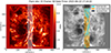 |
Fig. 3. Slit coverage over the slit-jaw image in Si IV 1400 Å (left) and Mg II (right). The pixel colours on the right represent the rejected (light blue) and retained (orange) spectra for a threshold in reconstruction error, and black any spectra that were removed during the preprocessing. To filter all observations from QS type spectra, we compared the retained areas in different observations. We have chosen the reconstruction threshold of 0.15, depicted here. |
2.4. Model training, validation, testing, and performance metrics
Our aim is to develop models that classify single spectra based on their shape if they belong to a PF or an AR observation. The classification models were trained on spectra combined from both the blue and yellow group of observations, otherwise the number of observations to create representative models would be too low. We test the models on unseen observations of either group to investigate flare precursors dependent and independent on X-ray flux. We used several metrics to infer model performances and to make them comparable to other studies. The raw model outputs which we denote henceforth by  do not correspond to a probability in the sense that the network would have learned the true probability of a certain spectrum appearing before a flare. However,
  relatively corresponds to probabilities in the sense that the higher the network output
  , the more likely the spectrum belongs to a PF observation. Comparing the true probability distribution to the distribution of the network outputs, one finds generally the network to be overconfident in its predictions (Guo et al. 2017). For example, the network’s output for a sample belonging to the positive class is higher than the actual probability that the sample belongs to the positive class.
In general, our raw model outputs are rounded to zero and one, with a distinguishing threshold of δ = 0.5, and compared to the true labels y = (0, 1, …, 1) to get the true positives TP  , true negatives TN
  , false negatives FN
  , and the false positives FP
  , defining the confusion matrix. We used P = TP + FN as the number of positive labels and N = TN + FP as the number of negative labels.
From this we used the metrics presented in Table 3 to compare the different models. We focussed most on the TSS since it is a class imbalance invariant metric and easy to interpret. TSS was first used in solar flare forecasting by Bloomfield et al. (2012). We verified following the example of Panos & Kleint (2020) by using the area under the receiver operating characteristic (ROC) curve (AUC), that a decision threshold of 0.5 is the best choice in our case. AUC is computed from the true positive rate TPR and the false positive rate FPR, where f1 and f0 stand for the distribution of the outputs assigned by the model to the spectra of the positive and negative classes (see Fig. 4). Such plots can be used to visually verify the correct choice of the classification threshold δ. If the two distributions are separated further away from δ = 0.5, the classification threshold needs to be adjusted towards the lowest overlapping point of the two distributions. We also computed the ROC skill score (ROCSS) since ROCSS provides easier interpretability than AUC. ROCSS is interpreted similarly to the TSS, but it is independent of the choice of the decision threshold δ, as it is derived from the AUC. In general, ROCSS is calculated as the difference between the AUC of a model in question and the AUC of a reference model, divided by the difference between a perfect model (AUC = 1) and the AUC of the reference model. The reference model can be, for instance, the climatological rate of occurrence of the phenomenon in question. In our case, the AUC of the reference model is set to 0.5, given that we impose strict class balance between the number of positive and negative spectra. Therefore, ROCSS simplifies to ROCSS = 2 ⋅ AUC − 1, as listed in Table 3.
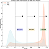 |
Fig. 4. Distributions assigned by a model to the PF and AR spectra over an entire validation set. The greater the overlap between the two distributions, the worse the AUC score becomes. |
Metrics to estimate the model performance.
Cohen’s kappa κ (Cohen 1960) in case of binary classification is equivalent to the Heidke Skill Score (Heidke 1926) also used by for instance Bobra & Couvidat (2015) to compare model performance. TSS is the only metric remaining constant under class imbalance and symmetric in the labels, as long as the scoring rates for the classes are kept constant. This can be demonstrated by replacing the false positives FP by N−TN and rewriting the TSS as:
 (1)
(1)
Changing the ratio between N/P in this case would not alter the TSS, since TP/P, TN/N = const are decoupled from N/P. The TSS reflects the ability of the model to make correct predictions per class, regardless of the size of each class. Cohen’s kappa is also mostly robust under class-imbalance, but not constant and normalises the output score to the class ratio through a hypothetical score under random guesses. We show the behaviour of the different metrics under different ratios of N/P between zero to 1000 and the rates TN/N = .6, and TP/P = .8 in Fig. 5.
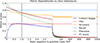 |
Fig. 5. Metrics’ dependencies on class imbalance. TP/P was selected as = 0.8 and TN/N = 0.6. N/P was varied between [0,1000]. The metrics vary in some cases drastically with changing N/P ratio. |
It shows that the TSS and Cohen’s kappa become similar around the point of balanced classes N/P = 1, but Cohen’s kappa decreases outside of balanced classes, keeping the rates TP/P and TN/N constant, while Precision, Accuracy and F1 still increase towards smaller N, but decrease for greater N. Recall remains constant but does not account for misclassification of negative examples except if we redefine it to reflect the performance on the negative class.
If a model cannot learn any inherent structures in a dataset, it will reflect the frequencies of both classes through random guessing. In case of extreme class imbalance, the model might still perform well in terms of accuracy, recall, precision and F1, though in terms of TSS and Cohen’s kappa it would return zero and reflect the inability of making true predictions. However, assuming the model is randomly guessing only on the negative class with a 50% chance, but scores perfectly on the positive class, we would get a similar TSS as presented in Fig. 5, although we could argue that in case of N ≪ P the model’s performance is much worse than in the case of N ∼ P.
Therefore and to ensure that our model learns the difference in spectral shapes independently of the natural size of the two classes, we subsampled the majority class and enforced near class balance during training. To investigate the behaviour of single observations, we used the raw model outputs and the aggregated TPR or FPR from all models not trained on the observation in question. To investigate the influence of subsampling the majority class on the models and scores, we trained a set of models without subsampling, ignoring class imbalance and we found that the scores with three different types of models are the same as for a subsampled dataset. To estimate our model’s performances we used the above introduced metrics, however, for our discussion only the accuracy and TSS are relevant. The complete set of scores computed in this study is presented on https://zenodo.org/records/11551490, and for sanity checks we always made sure that the different scores were not deviating qualitatively. The performance of our models is also determined by the observational splits between train, test, and validation sets. We chose stratified k-fold cross-validation to generate our train and validation splits with k = 5 folds and a number of repetitions of n = 5. This means we prepared five different disjoint validation sets of observations containing always the same number of observations at a ratio of 1:5 for validation and training. Repeating this process five times provided us with 25 samples to estimate our model performance. We assumed that the performance of each model is normally distributed around the true performance of a hypothetical model classifying any new observation. We estimated the true performance through the mean and standard deviation of our trained models’ performances on the different testing sets. To make sure our sample size is large enough, we computed the 95%-confidence interval for the true performance from our computed mean and standard deviation. With 25 models we got a relative accuracy of ∼5% which is good enough for our purpose.
Although it is standard in the field of machine-learning to have a separate test set on which the true performance of the models is estimated, we could not directly do the same. Since the spectra are labelled by observation and not by pixel position in the observations, for each choice the computed scores can be biassed by the observations in the testing set and their properties such as flare location, coverage by the slit, etc. Only estimating the true scores with many different splits between training and testing sets can alleviate this bias and account for the differences between observations.
Nevertheless, we could perform a similar approach as having a completely unseen testing set by splitting our data into two groups. Group one contains observations used in Panos & Kleint (2020) and group two contains the new observations added for this study. We trained models on both sets, estimated the model performance through stratified k-fold cross validation and tested the performance on the other untouched set as our testing set. Lastly, we combined group one and two, and only used the stratified k-fold cross validation to estimate the model’s performances.
2.5. Selection of model architectures
To train models we tested several different architectures and present the highest performing model architectures we found. The tested architectures are presented on https://github.com/jonaszubindu/IRIScast.git2. To the best of our knowledge no studies have focussed on the optimal machine-learning approach to identify pre-flare spectra and therefore we investigated potential alternative models to neural networks, such as the XGBoost (Chen & Guestrin 2016) decision trees.
The XGBoost algorithm is a light weight graph-based alternative to a neural network, and performs classifications by constructing a series of weak classifiers that are guided in a gradient descent like manner via the construction of binary trees (Chen & Guestrin 2016). Boosted trees achieve state of the art performance on many classification tasks with the added benefit of being more interpretable than their deep learning counterparts through the calculation of Shapley values. The concept of Shapley values was first introduced in cooperative game theory as a way to fairly distribute rewards amongst a coalition of players (Shapley 1951). The Shapley value can be directly mapped onto a machine-learning classification problem to rank the importance of input features and thereby give a way to interpret the importance of each input feature. Another prominent type of classifier would be a Support Vector Machine (SVM), for example applied by Bobra & Couvidat (2015). SVMs do not take correlations between features into account, which decision trees as well as deep learning based classifiers do, and they are therefore superior to SVMs. The standard components used in a fully connected neural network (FCNN) are depicted in Fig. 6. In each experiment with a single spectral line we compared four different architectures, which consist of an input layer and one, two, and three fully connected hidden layers, and in case of the fourth network a convolutional neural network (CNN) with two convolutional layers, and one, or two hidden layers. The best model architectures were determined through trial and error before performing a full scale experiment to estimate the true model performance.
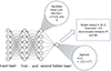 |
Fig. 6. Scheme of a standard fully connected neural network architecture, with its activation functions and output activation. |
2.6. Models trained on the combined dataset of Mg II h&k, Si IV, and C II
To combine the spectral lines into a single model architecture we used three different approaches. In the first approach we used a fully connected neural network. The second approach applies neural networks and XGBoost to features derived by the convolutional layers from our CNNs trained on single spectral lines. In our third approach, we concatenated the three spectral lines into one vector and trained a CNN, with three convolutional layers, and one, two, and three hidden layers. The models were applied to the combined dataset of the three spectral lines, such that each spectral line was present in each pixel. For instance, pixels used for Mg II h&k not reaching the minimum signal to noise ratio in Si IV or C II were excluded. Therefore, the combined dataset is the intersection between the pixels used for Mg II, Si IV, and C II, and is smaller than the dataset for each individual spectral line.
3. Results
This section is divided into 3 parts. First, we present the pre-flare spectra identification performance of neural networks trained on the individual spectral lines, Mg II h&k, Si IV, and C II. We conducted three different studies for each line and present the best scores obtained with the best model architecture. Secondly, we combined the three spectral lines and compare the scores of the models with a baseline threshold of only training models on Mg II h&k pixels from the combined dataset. The combined dataset does not contain the same pixels as the dataset for each individual spectral line (see Sect. 2.6), and therefore the baseline model has a different score than the models trained on all the spectra present in Mg II h&k. Thirdly, we used XGBoost decision trees on the network outputs from the models trained on individual spectral lines to rank the spectral lines according to the Shapley values computed for each model of each spectral line. The XGBoost decision trees are trained to predict from the  model outputs from the combined dataset which class a pixel belongs to, thereby taking the range of the
  model outputs into account. For instance, XGBoost could learn that when the model output from Si IV and C II is neutral (0.5) and from Mg II is positive (> 0.5) it still may be more likely for the investigated pixel to belong to the negative class. The trained XGBoost decision tree ensemble would thus detect an overconfidence for the models trained on Mg II. Upon finding such correlations, the scores from the XGBoost decision tree ensemble would improve compared to just evaluating the scores for each individual line for the same pixels. We did not find any improvement and therefore we conclude that the XGBoost decision trees only ranked the spectral lines according to how much information they cover for the identification of pre-flare spectra.
3.1. Estimate of true model performance
The architectures for the neural networks used in this study can be found on https://github.com/jonaszubindu/IRIScast.git3. In 12 out of 15 cases, the best performing architecture was a convolutional neural network. The complete results of all four architectures are presented on https://zenodo.org/records/11551490. For comparison to other studies, we focus only on two metrics, the accuracy and the TSS. The resulting scores are presented in Fig. 7. We have also observed that the differences in the scores between the four architectures are small. The maximum difference in TSS between the best and the worst performing architecture was ∼0.05. In the first panel we present the scores of the models trained on observations of group one, cross validated on group one and tested on the observations from group two. The models trained on Mg II h&k performed the best out of the three lines, followed by C II and Si IV. In each case of the three spectral lines the models perform worse on the testing set than on the cross validation set by about 0.1 − 0.3 in TSS.
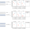 |
Fig. 7. Results from three different experiments to estimate the performance of the trained models generalising on unseen data. Models trained on Mg II h&k perform best in all experiments, followed by the models trained on C II and then Si IV. Contrary to Si IV and C II the performance on each dataset remains similar in the first two experiments, while the models trained on Si IV and C II always perform better in the cross validation, indicating some level of overfitting in case of the two FUV lines. |
In the second panel we repeated the same experiment but swapped groups one and two. The models in the second panel were trained on the observations from group two, cross validated on group two and tested on group one. In the case of Mg II h&k the models scored better on the testing set than in the cross validation, contrary to the results in the first panel. In case of Si IV we get similar scores to what we present in the first panel, with the models performing better in the cross validation than in the testing case. In the case of the models of C II the scores are low in both the cross validation and the testing. In the third panel we present the scores of the models trained on observations both from group one and two. For those models we do not have a separate testing set and only have the scores from the cross validation. Again, the models trained on Mg II h&k perform better than the models trained on Si IV and C II, where the latter reach similar scores.
In the case of Mg II h&k we surprisingly observe that the overall performance of the models are not the same on both sets of observations. It does not matter on which set the models were trained on, the scores remain similar for each group, which indicates inherent differences in the observations. We have also investigated the TPR and FPR for each observation and compared them between models trained and applied to non-VAE preprocessed observations and VAE preprocessed observations. We find that for Mg II h&k the scores improve with the preprocessing of removing quiet Sun spectra with a VAE by about 0.05 in TSS.
In case of Si IV we have found that we reach the best scores by applying an intensity mask of 3 × 10⁴ erg s−1 cm−2 sr−1 Å−1 to the observations. We have compared our scores with models trained on the same pixels in each observation as were used from the Mg II h&k observations, but have found only lower scores. For C II we have performed the same analysis as for Mg II h&k and Si IV, and reached the best scores by applying the same mask as was used for Mg II h&k, with the VAE preprocessing. We see a similar behaviour between the models trained on C II and on Si IV. The models perform in general better in the cross validation than when tested on the unseen data.
To understand if the difference between the scores of group one and two comes from observational bias (in case of models trained on Mg II h&k, but also in case of the other spectral lines), we have computed the linear correlation coefficients between the True (False) positive rate (TPR, 1 – FPR) for each PF (AR) observation with the heliocentric angle, cadence, solar-y coordinate, exposure time, the number of spectra after preprocessing the observation, the number of spectra after removal of quiet Sun like spectra with the VAE, the total time observed before the flare, the ratio between the spectra left after VAE and the original number of spectra in the observation, the active region number, the number of raster positions, and flare class. We have not found any significant correlations above 0.3, and therefore conclude that the discrepancy in the results can only come from the following options: (1) the type of spectra left in the observation after preprocessing and filtering spectra with the VAE, (2) the position of the slit in regards to where the flare occurs, (3) the physics of the flare and the pre-flaring atmosphere itself.
We repeated the same analysis with the models trained on Si IV and C II. In case of the models trained on C II observations from group one and tested on group two, we have found two correlations worth investigating: A correlation of 0.56 between the mean scores in TPR or (1 – FPR) and the ratio between the spectra deleted and the total number of available spectra, and a correlation of −0.76 between the mean scores in TPR or (1 – FPR), and the active region number. The first correlation implies a weak relation between observations with a higher number of spectra deleted during the preprocessing and a better score in classifying spectra from that observation. The second correlation implies that the classification scores worsen with increasing AR number, however, we do not expect this correlation to be causal in any way. We have found a correlation of 0.65 between the labels of the observations and the ratio of spectra deleted and the total number of spectra. However, we have not found such a correlation between the scores and the ratio of deleted spectra to total number of spectra in any other case. In the case of the FUV lines, this could come from an intensity bias, leading to the hypothesis that the models only learned the intensity information from the spectral shapes.
To test this hypothesis, we investigated the correlation between intensity and the network outputs of the models. We computed the Pearson correlation coefficient (Pearson 1895) between the intensity and the network outputs and found a weak correlation of ∼0.6 in all lines. We computed the coefficient of determination R2 of a linear fit between the two variables for each spectral line, and found ∼0.36, indicating that the intensity is not sufficient for flare forecasting. We can further support this claim by applying XGBoost to the intensity of all three spectral lines. We have reached an average accuracy score of ∼0.6 and a TSS of ∼0.25, which discredits the claim that the models only leverage intensity information for flare forecasting.
To also validate the use of neural networks directly on the spectral data instead of pre-selected features, we have trained XGBoost classifiers on the same pre-computed features as were used in Panos & Kleint (2020) for Mg II h&k. We also computed features derived from the Mg II h&k spectra, such as peak ratios, Doppler shifts, etc. and computed such features for C II and Si IV. For Si IV we computed the line centre, the line width, the line asymmetry, the Doppler shift of the line core, and the intensity. For C II we additionally computed the height of the central reversal, the ratio of the 1334.54 Å and the 1335.707 Å heights, the peak ratios around the central reversal, and the peak separation. We trained and cross validated 25 XGBoost classifiers on the observations in group one. The ones trained on Mg II h&k reach a TSS of 0.63, the ones trained on Si IV a TSS of 0.11, and the ones trained on C II a TSS of 0.37. We repeated the same analysis while training neural networks on the feature dataset and achieved very similar scores. For Mg II h&k we reached a TSS of 0.62, for Si IV a TSS of 0.05, and for C II a TSS of 0.36. The scores found through training on precomputed features are all below what could be achieved with neural networks directly trained on the spectral data.
3.2. Combining spectral lines for precursor classification
To test whether pre-flare spectra can be better identified by combining the information from multiple spectral lines, we carried out two studies. In the first study we used a CNN on three spectra Mg II, C II, Si IV) from each pixel in the combined dataset concatenated together. The model architecture consisted of two convolutional layers and two hidden layers. In our second study we used the feature outputs from the convolutional layers of the trained CNNs of the single spectral line study (see Sect. 3.1), which we refer to as self-learned features. Since for each spectral line individually the convolutional neural network had in general the best performance, we used only CNN based architectures for these two studies. In the case of the second study, we anticipate the self learned features contain the highest amount of information from the individual spectra for finding flare precursors. The remaining task is then to combine this information and find the information shared between the lines, which is done by training a NN on the self learned features at classifying the pixels.
In Fig. 8 we show the results of study one (centre panel) and study two (right panel). Since the pixels from the single spectral line and the combined dataset are different, the scores cannot be compared directly to the results in Fig. 7. To obtain comparable scores, we had to retrain the NN-models on the Mg II h&k pixels from the combined dataset (left panel), using the self-learned features from the Mg II h&k single line CNNs as a baseline.
 |
Fig. 8. Model performance estimated through cross validation for the combination of Mg II h&k, C II, and Si IV. As baseline for comparison we have used Mg II h&k (left panel), reaching a lower TSS than in the single line experiments with VAE preprocessing. In the experiments with the completely newly trained convolutional neural network (centre panel) and the pre-learned features (right panel) for the line combination we can observe an increase compared to the baseline experiment with Mg II h&k. |
Both studies combining the three spectral lines reach slightly higher TSS and accuracy than the Mg II baseline scores. Both studies (centre and right panel) are very similar, however, the right panel shows a wider distribution in model scores. Therefore, the combination of information can improve the separation of PF and AR spectra. However, the intersection of pixels in all three spectral lines produces lower scores compared to the models trained on the single spectral line dataset of Mg II h&k.
3.3. Ranking spectral lines in terms of precursor classification power
As explained at the beginning of Sect. 3, the XGBoost decision tree classifier should learn which outputs and which spectral lines have the most distinctive features, and rank the spectral lines accordingly. We repeated this experiment on the same train-test-splits as the NN-models were trained and tested on, and used the combined dataset of the three spectral lines. Thus, we trained 25 decision tree classifiers and ranked the spectral line model outputs by computing their Shapley values and investigated the result in beeswarm-plots. For all but one split (C II ranked highest in one split) we find that Mg II h&k line is the most distinct spectral line to distinguish PF and AR spectra, followed by C II in 23 splits and the lowest ranked line is Si IV. This is in agreement with the performance results we got for each line individually in Sect. 3.1. One example of a split is presented in Fig. 9.
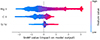 |
Fig. 9. Example plot presenting the ranked importance of each spectral line in terms of Shapley values. The y-axis gives the ranking of the spectral lines: Mg II h&k is ranked highest, followed by C II and Si IV ranked the lowest. The width of the horizontal features is proportional to the number of occurrences, for example, most Shapley values for Si IV were between zero and 0.2. The range of the Shapley values was largest for Mg II, which is visible as the extent of the x-axis. The colour indicates the magnitude of the network outputs of the models, while the Shapley values indicate the direct impact on the XGBoost model output. The colour corresponds to the |

4. Discussion
4.1. Single spectral lines solar flare precursor classification
We investigated whether Mg II h&k, Si IV, or C II spectra are most suitable to distinguish PF and AR spectra, which could have an application for flare forecasting. The best results were obtained with models trained on Mg II h&k, preprocessed with a VAE to remove quiet Sun spectra. The best model architecture was a convolutional neural network in all three line experiments. This can be explained by the inherent capability of CNNs automatically finding spatially correlated features within the input and performing classification based upon the presence, absence and strength of those features. Fully connected neural networks do not have this ability and only learn the correlations between the strength of features, whereas each input node becomes a feature. We verified if a purely handpicked feature based approach performs better than using the spectra directly as inputs and have found that the latter performed consistently better. This implies that the CNNs have found additional features to the ones selected by Panos & Kleint (2020) and used in this study as comparison, which is in agreement with the findings of Panos et al. (2023).
We have found that the model scores differed, depending on which observations were in the testing set. This indicates that some observations may be better for finding distinct flare-precursors than others. This is understandable, considering that IRIS is a slit spectrograph and the slit with its limited spatial extent is not guaranteed to cover the full flare.
The fact that the models trained on Mg II performed consistently under the exchange of the training and testing set indicates that even in the sample where possibly some observations were less flare-indicative, there were sufficient other flare-indicative spectra. The models thus were able to learn more general information encoded in the shape of the spectra to distinguish the pre-flaring atmosphere from the active region atmosphere. The Si IV and C II lines scored worse. However, they also had to be trained on fewer pixels because of lower signal to noise ratio. This could mean the FUV lines did not contain enough representative observations to obtain the full distribution of the PF and AR information, or the spectral shape does not contain many flare precursors. The model scores found for Mg II h&k with the models trained and cross validated on observations from group one are higher than what was previously reported in Panos & Kleint (2020), however, the scores found in the cross validation on groups one and two together reach a similar level as found in Panos & Kleint (2020).
It is remarkable that Mg II h&k is the spectral line with the most distinguishing spectral shapes, and the network outputs are often high during the entire one hour pre-flare phase. For some observations we observed even longer duration of high probability, without observing clear trends towards flare onset. A recent study investigating flare precursors based on several spectra together in a multiple-instance learning approach have observed high probability areas in one observation for more than 5 hours (Huwyler & Melchior 2022). These results imply that pre-flare signatures can be present several hours before flare onset. In our study of the Mg II h&k line we observe the same behaviour for longer observations with a high probability over the entire observation duration.
Characteristics of the Mg II spectra, both in the h&k line cores and deep wings, and also in the 3p−3d ‘triplet’ lines all exhibit behaviour flagged to predict an imminent flare (Panos & Kleint 2020; Woods et al. 2021; Huwyler & Melchior 2022; Panos et al. 2023). Stronger emission cores and emission in the triplet of lines all indicate enhanced temperatures (and perhaps densities) in the upper chromosphere, from elementary considerations: The 3p level populations must be enhanced to produce stronger emission in the h&k lines and more opacity in the triplet lines, and the 3d levels must also be enhanced to produce emission lines. Both vary as exp(−E/kTe) with E = 4.43 and 8.86 eV respectively, and Te ≡ 0.6 eV in the chromosphere. Sophisticated calculations (albeit for quiet Sun conditions, Pereira et al. 2015) limit the enhanced temperatures in the upper chromosphere (column densities below 10−4 g cm−2). The worse capabilities of C II and Si IV at distinguishing spectra from PF and AR observations suggests that processes are occurring in plasma below the typical transition region, that is in plasma that is not completely ionised. The two FUV spectral lines do not contain information about the continuum, nor about the lower to mid chromosphere.
4.2. Combining spectral lines to improve model classification performance
If the two spectral lines Si IV and C II contained complementary information to Mg II h&k for flare prediction, combining spectral lines should increase the score of the models. The drawback of this study was that fewer pixels and thus fewer different spectra could be used to train the models because of the combination of our S/N criteria. We compared the models trained on the line combinations to a baseline threshold of models only trained on Mg II h&k. The scores improved when the three spectral lines were combined (see Fig. 8). However, the difference between using the combination of all three lines with various setups or only Mg II is not large. Therefore, we conclude that there is some complementary information not shared by the lines, which can improve the model scores. However, we have not observed overall better results than in case of training models on the VAE preprocessed observations in the Mg II h&k line as discussed in Sect. 4.1, where more pixels and spectra were used to train the models. This could imply that either the most important information from Mg II h&k is in pixels where Si IV or the C II line did not have sufficient S/N, which led to the pixel being excluded during the combined study. Another possibility is that on a statistical basis more unnecessary pixels ‘dilute’ the model scores, especially because we labelled each spectrum or pixel only with the respective type of observation (PF, AR). In terms of physics, it is possible that the large formation height range of Mg II is already sufficient for finding the most relevant flare precursors and the height ranges covered by the Si IV and the C II lines do not contribute significant new information. This is also reflected in the line ranking study with XGBoost, where the Mg II h&k was consistently ranked highest. Additionally, as can be seen in Fig. 9, the network outputs from the Mg II line were assigned the highest absolute Shapley values, meaning the relative focus of the XGBoost decision tree was highest on the Mg II network outputs.
4.3. Label noise and flare class
Due to our choice of labelling all spectra by the type of observation they occur in, we encountered the following problems: Firstly, we have an overlap of PF spectra in AR observations and AR spectra in PF observations and the model can only learn to distinguish the two on a basis of frequency per observation. Secondly, we are dealing with a continuum of shapes and not a strict binary system as would be the case for instance in classifying pictures of cats and dogs. Thirdly, the pointing of the satellite may affect our results. Assuming we have a PF observation with the spectrograph slit covering 20% of the flare and maybe only recording the tip of one of the flare ribbons, we cannot be sure that the slit recorded enough PF signatures for our model to flag that observation as PF in a hypothetical real-time application.
Additionally, since we have not found any correlation between flare class and TPR we can conclude that on a spectral level flares are scale invariant. One example directly supporting the two last arguments is PF-observation two. As depicted in Fig. 10 the slit position covered the area well where the X1.0 flare occurred. Nevertheless, the pre-flare signature was limited to a small area on the slit and therefore the observation scores low. Thus, in general PF spectra of a < C5 class flare do not differ from > C5 class PF spectra, neither in shape nor in frequency within one observation.
 |
Fig. 10. PF-observation number two, which resulted in an X1.0 flare. The active region is limited to a small area of the IRIS spectrograph slit. The models flag the area above the polarity inversion line as most important. |
On the opposite hand, if we have an observation of an AR, we can still have small flare kernels (≪C5), and if the slit exactly covers a small region with reconnection or heating, producing similar kernels to the learned pre-flare kernels, and persistent over several tens of minutes, then an AR observation can be misclassified as PF. An example of which is shown in Fig. 11. In the selected frame, a small eruption, identified in HEK as a C4.2 flare, is visible. Therefore it is likely that the model identifies the area as pre-flaring. This flare was not listed in our initial flare list with all flares observed by IRIS, and was also labelled as an AR observation in Panos & Kleint (2020), Panos et al. (2023), we only noticed the coincidence after our analysis.
 |
Fig. 11. AR-observation 16. A small flare erupted that was not in the flare list and only later noticed. Our model successfully tracks the area where the small flare occurs throughout the entire observation, before, during and after the eruption. |
We also compared the area of high probability for a flare in Mg II with continuum, magnetogram, and AIA 304 images. We chose to present AIA 304 since the 304 channel covers the emission of He II, which forms in the chromosphere and transition region, similar to Mg II. Fig. 10 and the upper panel of Fig. 12 display how the areas with the strongest magnetic fields and especially around the polarity inversion lines are showing the highest probability on the slit. Conversely, we have also found examples where the area in between patches of strong magnetic fields and polarity inversion lines can exhibit high probability for a flare in Mg II, one such example is presented in the lower panel of Fig. 12. In contrast to the upper panel of Fig. 12, it is clearly visible that the area of high probability is not only overlapping the regions of penumbral filaments but is actually highlighting a large area unassociated with the photospheric magnetic field as important. This means that Mg II is also sensitive to processes related to flares happening in the chromosphere that cannot be directly attributed to the magnetic field structure in the photosphere. Therefore, we conclude that Mg II spectral data and photospheric magnetic field data have shared information, but are not completely correlated.
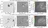 |
Fig. 12. PF observation 34 (upper panel) and PF observation one (lower panel) showing the areas of high probability in comparison with the continuum, the magnetogram, and the AIA 304 channel of SDO. In the upper panel the area of high probability flagged by our models spans the entire area of increased magnetic field but also extends beyond the edges of the penumbra. In the lower panel we also see how the area of high importance spans over the areas of strong magnetic fields but additionally covers the area in between, where the photospheric magnetic field is weak. |
Since we have trained our models on single pixels, the pixels between the strong magnetic field patches do not have any information about the pixels above the strong magnetic field patches or the polarity inversion line and must contain some information limited to the chromosphere, that is indicative for the pre-flaring atmosphere. Compared to the images in AIA 304 we see loop structures, brightenings, and filaments in all of them, but there is no apparent pattern between the high probability area on the slit and these structures. For instance, in the upper panel of Fig. 12 the observed filaments and loops are somewhat correlated to the network outputs, however, also areas in between these structures are flagged with high probability to be flare related. Some parts of the extensions in the lower part of the slit where loops are present are even flagged with low probability. We have also performed the same comparison with other AIA channels, but did not find any apparent patterns. This again suggests that our models learned information about the state of the chromosphere resolved with height from the spectral shapes.
4.4. Misclassification of single observations and influence of X-ray flux precursors
To investigate reasons for misclassification using models trained on Mg II h&k we collected the misclassified observations by TPR and FPR, meaning we have computed the average TPR (PF) and FPR (AR) for each flare by using all models not having the associated observation in its training set. We compared slit coverage, flare class, and flaring area, and have found that out of 18 misclassified flares three flares have a bad slit coverage, three flares have many raster steps and span a too large area, seven flares have a very faint or few pre-flare kernels, but are in the right position where later the flare appears, and for five observations we are unable to determine any special features that may explain their misclassification (one PF and four AR). This could be mitigated by having standardised sets of observations, especially in a potential future real-time application.
Lastly, we have investigated the dependency of the precursors our models find on X-ray flux events recorded with GOES. For this we used the TPR of each PF flare and compared them between groups blue and yellow. The TPR is in general the same in both groups, and no obvious difference can be noticed. Group blue contains 21 PF samples and group yellow contains 52 PF samples. For Mg II h&k we have found 5 misclassified flares from group blue, and 6 misclassified flares from group yellow. For Si IV we have found 12 from group blue, and 12 from group yellow, and for C II we have found seven from group blue, and 6 from group yellow. In case of Mg II h&k two of these flares have a bad slit coverage, and one flare has many slit positions to cover the pre-flaring area. Leaving two flares without explanation for the misclassification in group blue. In group yellow two flares have too many slit positions, and three flares have a bad slit coverage, leaving two flares without explanation. Thus, the rate of misclassifications is by a factor two higher for group blue. We can conclude that the difference between the scores does in general not depend on the X-ray flux and the models are picking up signals uncorrelated to X-ray flux as well as signals correlated to X-ray flux.
5. Summary and conclusions
We presented an extensive analysis of distinguishing PF and AR spectra, which may lead to future flare prediction capabilities. We considered different neural network architectures, finding the best architecture to be a convolutional neural network. We also tested the application of different masks to improve robustness of our models, such that the models only focus on the active areas within each observation. The models trained on Mg II h&k preprocessed with a VAE to remove quiet Sun type spectra reached the highest scores and exceeded previously reported scores in TSS on the same dataset (Panos & Kleint 2020). We could show that the models robustly learned to identify pre-flare signatures independent of observational properties, or GOES X-ray flux. We speculate that pre-flare signatures may be present in the lower solar atmosphere and are better captured by Mg II with its large formation height range. However, certain observational properties and the choice of labelling each spectrum by the type of observation they occur in influences the final scores and makes it harder to compare reliability of the models for a potential future real-time application.
The flare class had no influence on the overall scores of an observation. We observed that in AR observations areas with small eruptive events not considered as a flare are also flagged with high probability by our models, which may be physically correct, but impacts the scores negatively. On the other hand, some of the bigger flares were ideally located in the FOV, but have not scored high for that particular observation because the flaring area was concentrated only on a small part of the slit.
We investigated the relevance of intensity in an active region (intensity in the individual pixels) and have found a weak correlation, as well as low scores for models trained only on the intensity value. Therefore, it is evident that the spectral shape is more important to understand the pre-flaring atmosphere than what could be understood from intensity alone. Because we have found the same for all three spectral lines we suspect that the intensity light curves observed in AIA are most likely also carrying little information to understand the pre-flare atmosphere and spectral information has to be taken into account.
Comparing the areas of high probability outputs of our models with the photospheric magnetic field we cannot see an apparent correlation between the two. The same applies to structures observed in AIA 304. We also investigated the other AIA channels for apparent patterns between the Mg II and structures observed with AIA and have not found any apparent correlations, however, no quantitative analysis was performed. The models trained on Si IV and C II reached scores only slightly lower to what has been reported for Mg II h&k previously. However, we observed certain effects of overfitting for Si IV and C II implying that our dataset might not be representative enough for finding precursors with machine-learning in Si IV and C II and would have to be extended. Training models on the combination of spectral lines has turned out to be difficult due to the difference in areas of importance between the different lines, but could improve the scores in case of an ideal selection of pixels for all three lines. From these conclusions we can draw three potential improvements for future research:
-
By increasing the number of observations one could train models on the basis of entire observations, which would be beneficial to mitigate observational bias, as well as selection of pixels within each observation.
-
The observed time before a flare is rather short to make a statement about the utility of spectra for longterm solar flare forecasting. However, we have observed that the model outputs in the PF observations remain high in most observations during the entire one hour duration before the flare, suggesting that the precursors learned by the models are present longer than one hour before flare onset.
-
Past studies have shown the potential of using magnetic field data for flare prediction, and the present study highlights the importance of height resolved information about the solar atmosphere in solar flare forecasting. Thus, a space-based observatory combining magnetic field data of the chromosphere, the photosphere, as well as spectra encoding the physics of the solar atmosphere resolved with height and high cadence would be the ideal observatory to attempt real-time solar flare forecasting (Judge et al. 2021).
This work represents a step into the direction of utilising spectra-based solar flare prediction algorithms, making use of the height dependent information about the physical properties of the solar atmosphere. It may help to guide the design of future space-based observatories that have the aim to provide a rich dataset to solve the flare prediction problem in a real-time application scenario.
Acknowledgments
This work was supported by a SNSF PRIMA grant. We are grateful to LMSAL for allowing us to download the IRIS database. IRIS is a NASA small explorer mission developed and operated by LMSAL with mission operations executed at NASA Ames Research Center and major contributions to downlink communications funded by ESA and the Norwegian Space Centre. This research has made use of NASA’s Astrophysics Data System Bibliographic Services. Some of our calculations were performed on UBELIX (http://www.id.unibe.ch/hpc), the HPC cluster at the University of Bern. We are also very thankful for the insightful discussions with Dr. Philip Judge about line formation of Mg II h&k.
References
- Bloomfield, D. S., Higgins, P. A., McAteer, R. T. J., & Gallagher, P. T. 2012, ApJ, 747, L41 [CrossRef] [Google Scholar]
- Bobra, M. G., & Couvidat, S. 2015, ApJ, 798, 135 [Google Scholar]
- Chen, T., & Guestrin, C. 2016, Proceedings of the 22nd ACM SIGKDD International Conference on Knowledge Discovery and Data Mining, KDD’16 (New York: ACM) [Google Scholar]
- Cheng, C. C., Tandberg-Hanssen, E., & Orwig, L. E. 1984, ApJ, 278, 853 [NASA ADS] [CrossRef] [Google Scholar]
- Cohen, J. 1960, Educ. Psychol. Meas., 20, 37 [CrossRef] [Google Scholar]
- De Pontieu, B., Title, A. M., Lemen, J. R., et al. 2014, Sol. Phys., 289, 2733 [Google Scholar]
- Deshmukh, V., Baskar, S., Berger, T. E., Bradley, E., & Meiss, J. D. 2023, A&A, 674, A159 [NASA ADS] [CrossRef] [EDP Sciences] [Google Scholar]
- Florios, K., Kontogiannis, I., Park, S.-H., et al. 2018, Sol. Phys., 293, 28 [NASA ADS] [CrossRef] [Google Scholar]
- Georgoulis, M. K., Bloomfield, D. S., Piana, M., et al. 2021, J. Space Weather Space Clim., 11, 39 [CrossRef] [EDP Sciences] [Google Scholar]
- Guo, C., Pleiss, G., Sun, Y., & Weinberger, K. Q. 2017, ArXiv e-prints [arXiv:1706.04599] [Google Scholar]
- Harra, L. K., Matthews, S. A., & Culhane, J. L. 2001, ApJ, 549, L245 [NASA ADS] [CrossRef] [Google Scholar]
- Heidke, P. 1926, Geografiska Annaler, 8, 301 [Google Scholar]
- Huang, X., Wang, H., Xu, L., et al. 2018, ApJ, 856, 7 [NASA ADS] [CrossRef] [Google Scholar]
- Hurlburt, N., Cheung, M., Schrijver, C., et al. 2010, Sol. Phys., 275, 67 [Google Scholar]
- Huwyler, C., & Melchior, M. 2022, Astron. Comput., 41, 100668 [NASA ADS] [CrossRef] [Google Scholar]
- Jonas, E., Bobra, M., Shankar, V., Todd Hoeksema, J., & Recht, B. 2018, Sol. Phys., 293, 48 [NASA ADS] [CrossRef] [Google Scholar]
- Judge, P., Rempel, M., Ezzeddine, R., et al. 2021, ApJ, 917, 27 [NASA ADS] [CrossRef] [Google Scholar]
- Kastner, S. O. 1993, Space Sci. Rev., 65, 317 [NASA ADS] [CrossRef] [Google Scholar]
- Kingma, D. P., & Welling, M. 2013, ArXiv e-prints [arXiv:1312.6114] [Google Scholar]
- Leka, K. D., & Barnes, G. 2003, ApJ, 595, 1277 [CrossRef] [Google Scholar]
- Leka, K. D., & Barnes, G. 2007, ApJ, 656, 1173 [NASA ADS] [CrossRef] [Google Scholar]
- Leka, K. D., Dissauer, K., Barnes, G., & Wagner, E. L. 2023, ApJ, 942, 84 [NASA ADS] [CrossRef] [Google Scholar]
- Lemen, J. R., Title, A. M., Akin, D. J., et al. 2012, Sol. Phys., 275, 17 [Google Scholar]
- McCully, C., Crawford, S., Kovacs, G., et al. 2018, https://doi.org/10.5281/zenodo.1482019 [Google Scholar]
- Nishizuka, N., Sugiura, K., Kubo, Y., et al. 2017, ApJ, 835, 156 [NASA ADS] [CrossRef] [Google Scholar]
- Nishizuka, N., Sugiura, K., Kubo, Y., Den, M., & Ishii, M. 2018, ApJ, 858, 113 [NASA ADS] [CrossRef] [Google Scholar]
- Panos, B., & Kleint, L. 2020, ApJ, 891, 17 [NASA ADS] [CrossRef] [Google Scholar]
- Panos, B., Kleint, L., Huwyler, C., et al. 2018, ApJ, 861, 62 [Google Scholar]
- Panos, B., Kleint, L., & Voloshynovskiy, S. 2021, ApJ, 912, 121 [NASA ADS] [CrossRef] [Google Scholar]
- Panos, B., Kleint, L., & Zbinden, J. 2023, A&A, 671, A73 [NASA ADS] [CrossRef] [EDP Sciences] [Google Scholar]
- Pearson, K. 1895, Proc. R. Soc. London, 58, 240 [NASA ADS] [CrossRef] [Google Scholar]
- Pereira, T. M. D., Carlsson, M., Pontieu, B. D., & Hansteen, V. 2015, ApJ, 806, 14 [NASA ADS] [CrossRef] [Google Scholar]
- Pesnell, W. D., Thompson, B. J., & Chamberlin, P. C. 2012, Sol. Phys., 275, 3 [Google Scholar]
- Schou, J., Scherrer, P. H., Bush, R. I., et al. 2012, Sol. Phys., 275, 229 [Google Scholar]
- Shapley, L. S. 1951, Notes on the N-Person Game; II: The Value of an N-Person Game (Santa Monica: RAND Corporation) [Google Scholar]
- van Dokkum, P. G. 2001, PASP, 113, 1420 [Google Scholar]
- Woods, M. M., Dalda, A. S., & Pontieu, B. D. 2021, ApJ, 922, 137 [NASA ADS] [CrossRef] [Google Scholar]
Appendix A: VAE to filter quiet Sun spectra
A VAE is an unsupervised generative model that consists of an encoder decoder model type architecture, as depicted schematically in Fig. A.1. Both the encoder and decoder functions are parameterised by neural networks eϕ and dθ respectively. The VAE samples spectra x and encodes them onto a low-dimensional latent space representation z. The latent space is restrained by a prior distribution to be a simple, easy to sample distribution, in this case a multivariate Gaussian P(z):=𝒩(0, 1). For each spectrum, the encoder computes a mean vector μ(x) and variance matrix Σ(x) to construct a normal distribution Q ∼ 𝒩(μ, Σ) close to the prior. The VAE then samples a latent variable z from the distribution Q, and the decoder network attempts to reconstruct the spectrum x′=dθ(z). The VAE is optimised such that the difference between the encoded and decoded spectrum is small, while maintaining an approximately Gaussian shaped latent space. To achieve this the VAE maximizes the full log likelihood
 (A.1)
(A.1)
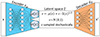 |
Fig. A.1. Schematic depiction of a VAE architecture with the sampling rule of the latent variable z from the distribution 𝒩(μx, σx), x represents the input spectrum, while x′ represents the reconstructed spectrum from z. |
which is proportional to the ℒ2-norm of the original spectrum x and the reconstructed spectrum x′=dθ(z′), later denoted as reconstruction error. The full loss function is given by
![Mathematical equation: $$ \begin{aligned} L = E_{x \sim D} [E_{\epsilon \sim \mathcal{N} (0, I)} [\Vert x-d_{\theta }(z)\Vert ^{2}] -\mathcal{D} \left[Q(z \mid x) \Vert P(z)\right]], \end{aligned} $$](/articles/aa/full_html/2024/09/aa47824-23/aa47824-23-eq19.gif) (A.2)
(A.2)
and 𝒟[Q(z ∣ x)∥P(z)] is the KL-divergence pulling the distribution Q closer to the prior P(z). z is sampled from the distribution Q through z = μ(x)+Σ1/2(x)⋅ϵ, sampling ϵ from 𝒩(0, 1). VAEs are bad at reconstructing out-of-distribution data. This means if we train a VAE on input spectra exclusively from QS observations, it will perform badly at reconstructing a spectrum typical for an AR or PF observation, which is not similar to a QS spectrum, and would result in a high reconstruction error. Therefore, we can use the reconstruction error as a threshold to clean observations from QS spectra and greatly reduce mixing of classes between QS and PF and AR spectra. The architecture used for our VAE and the training process can be found on https://github.com/jonaszubindu/IRIScast.git.
To select our threshold, we manually compared different options between many observations. In Fig. A.2 we show a comparison between three different reconstruction error thresholds and the selected area of the slit as active (in orange), overlaid on a frame with high activity just before the onset of the flare. In the left panel we used a threshold of 0.1. Almost the entire slit is covered in orange and thus the VAE would select too many pixels as active areas. The centre panel displays a threshold of 0.15, which follows the bright area plus some other active regions. In the right panel we used a threshold of 0.25, where we see the area on the slit is slightly more concentrated on the bright area than in the centre panel. However, we observed that in other PF and AR observations almost no pixels were selected by the VAE with a threshold of 0.25. Therefore, we subjectively chose a reconstruction threshold of 0.15 to remove most QS type spectra from our dataset.
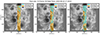 |
Fig. A.2. Comparison of three different reconstruction thresholds for a single observation, overlaid on the Mg II slit-jaw image. The light blue pixels are the spectra reconstructed with an error lower than the chosen reconstruction threshold. The pixels in orange are the spectra reconstructed with an error above the threshold. In the left panel a too low threshold was selected, most pixels are kept. The right panel shows how only areas around the bright ribbon like structure are selected and in the centre panel the bright structure and some areas extending around it are kept. |
All Tables
All Figures
|
Fig. 1. Examples of observations of active regions with IRIS in the continuum channel of HMI, the recalibrated GOES X-ray flux for the time period of the observation, and the flare class from the HEK database. The red frame with the vertical lines displays the FOV and the slit positions of the IRIS spectrograph. In the GOES X-ray flux we show the time window of the IRIS observation as a light blue shaded region. The red shaded region with the vertical line depicts the time of a flare, from beginning to end, according to the HEK database. The black dashed vertical and horizontal line depict the parts that were cut from the observations and used for training and testing the classification models. |
| In the text | |
|
Fig. 2. Example of IRIS spectra used for this study, showing the three considered spectral lines Mg II, C II, and Si IV. The IRIS spectrograph slit is visible as a vertical black line in the flare image at location x ∼ 370. |
| In the text | |
|
Fig. 3. Slit coverage over the slit-jaw image in Si IV 1400 Å (left) and Mg II (right). The pixel colours on the right represent the rejected (light blue) and retained (orange) spectra for a threshold in reconstruction error, and black any spectra that were removed during the preprocessing. To filter all observations from QS type spectra, we compared the retained areas in different observations. We have chosen the reconstruction threshold of 0.15, depicted here. |
| In the text | |
|
Fig. 4. Distributions assigned by a model to the PF and AR spectra over an entire validation set. The greater the overlap between the two distributions, the worse the AUC score becomes. |
| In the text | |
|
Fig. 5. Metrics’ dependencies on class imbalance. TP/P was selected as = 0.8 and TN/N = 0.6. N/P was varied between [0,1000]. The metrics vary in some cases drastically with changing N/P ratio. |
| In the text | |
|
Fig. 6. Scheme of a standard fully connected neural network architecture, with its activation functions and output activation. |
| In the text | |
|
Fig. 7. Results from three different experiments to estimate the performance of the trained models generalising on unseen data. Models trained on Mg II h&k perform best in all experiments, followed by the models trained on C II and then Si IV. Contrary to Si IV and C II the performance on each dataset remains similar in the first two experiments, while the models trained on Si IV and C II always perform better in the cross validation, indicating some level of overfitting in case of the two FUV lines. |
| In the text | |
|
Fig. 8. Model performance estimated through cross validation for the combination of Mg II h&k, C II, and Si IV. As baseline for comparison we have used Mg II h&k (left panel), reaching a lower TSS than in the single line experiments with VAE preprocessing. In the experiments with the completely newly trained convolutional neural network (centre panel) and the pre-learned features (right panel) for the line combination we can observe an increase compared to the baseline experiment with Mg II h&k. |
| In the text | |
|
Fig. 9. Example plot presenting the ranked importance of each spectral line in terms of Shapley values. The y-axis gives the ranking of the spectral lines: Mg II h&k is ranked highest, followed by C II and Si IV ranked the lowest. The width of the horizontal features is proportional to the number of occurrences, for example, most Shapley values for Si IV were between zero and 0.2. The range of the Shapley values was largest for Mg II, which is visible as the extent of the x-axis. The colour indicates the magnitude of the network outputs of the models, while the Shapley values indicate the direct impact on the XGBoost model output. The colour corresponds to the |
| In the text | |
|
Fig. 10. PF-observation number two, which resulted in an X1.0 flare. The active region is limited to a small area of the IRIS spectrograph slit. The models flag the area above the polarity inversion line as most important. |
| In the text | |
|
Fig. 11. AR-observation 16. A small flare erupted that was not in the flare list and only later noticed. Our model successfully tracks the area where the small flare occurs throughout the entire observation, before, during and after the eruption. |
| In the text | |
|
Fig. 12. PF observation 34 (upper panel) and PF observation one (lower panel) showing the areas of high probability in comparison with the continuum, the magnetogram, and the AIA 304 channel of SDO. In the upper panel the area of high probability flagged by our models spans the entire area of increased magnetic field but also extends beyond the edges of the penumbra. In the lower panel we also see how the area of high importance spans over the areas of strong magnetic fields but additionally covers the area in between, where the photospheric magnetic field is weak. |
| In the text | |
|
Fig. A.1. Schematic depiction of a VAE architecture with the sampling rule of the latent variable z from the distribution 𝒩(μx, σx), x represents the input spectrum, while x′ represents the reconstructed spectrum from z. |
| In the text | |
|
Fig. A.2. Comparison of three different reconstruction thresholds for a single observation, overlaid on the Mg II slit-jaw image. The light blue pixels are the spectra reconstructed with an error lower than the chosen reconstruction threshold. The pixels in orange are the spectra reconstructed with an error above the threshold. In the left panel a too low threshold was selected, most pixels are kept. The right panel shows how only areas around the bright ribbon like structure are selected and in the centre panel the bright structure and some areas extending around it are kept. |
| In the text | |
Current usage metrics show cumulative count of Article Views (full-text article views including HTML views, PDF and ePub downloads, according to the available data) and Abstracts Views on Vision4Press platform.
Data correspond to usage on the plateform after 2015. The current usage metrics is available 48-96 hours after online publication and is updated daily on week days.
Initial download of the metrics may take a while.