| Issue |
A&A
Volume 689, September 2024
|
|
|---|---|---|
| Article Number | A296 | |
| Number of page(s) | 14 | |
| Section | Stellar structure and evolution | |
| DOI | https://doi.org/10.1051/0004-6361/202347505 | |
| Published online | 19 September 2024 | |
Timing and scintillation studies of PSR J1439−5501
1
Max Planck Institute for Radioastronomy (MPIfR), auf dem Hügel 69, 53121 Bonn, Germany
2
Centre for Astrophysics and Supercomputing, Swinburne University of Technology, PO Box 218 Hawthorn, Vic 3122, Australia
3
ARC Centre of Excellence for Gravitational Wave Discovery (OzGrav), Swinburne University of Technology, Mail H11, PO Box 218 VIC 3122, Australia
4
South African Radio Astronomy Observatory, 2 Fir Street, Observatory 7925, South Africa
Received:
19
July
2023
Accepted:
26
April
2024
Abstract
Context. PSR J1439−5501 is a mildly recycled pulsar in a 2.12-day circular orbit around a heavy white dwarf. A white dwarf cooling model has estimated the companion mass to be between 1 and 1.3 M⊙ and the inclination angle to be greater than 55°. Such high mass and inclination are expected to induce a Shapiro delay, namely, a relativistic time delay in the signal propagation caused by the curved space-time induced by the companion. Until now, however, no Shapiro delay has been measured in this system.
Aims. Our aim is to detect the Shapiro delay and, thus, to independently measure the mass and inclination of PSR J1439−5501 by using data from the Parkes and MeerKAT radio telescopes.
Methods. The Shapiro delay parameters were measured through pulsar timing, which coherently accounts for every rotation of the pulsar. These measurements were then used to estimate the masses of the component stars and the inclination angle of the binary. A scintillation analysis was additionally performed by investigating the secondary spectra, which are the Fourier-transformed observed scintillation patterns. The obtained secondary spectral variations were analyzed in terms of the orbital motion and annual variation to estimate the ascending nodes, distance, and the location of the screen.
Results. We obtained a highly significant measurement of the Shapiro delay, which allows estimates of the pulsar mass (1.57−0.26+0.30 M⊙), the white dwarf (WD) companion mass (1.27−0.12+0.13 M⊙), and inclination angle, (75(1)° or 105(1)°). These estimates assume that the companion mass cannot exceed the Chandrasekhar mass limit (1.48 M⊙), along with a lower limit of 1.17 M⊙ for NS masses. These results are consistent with previous studies, but the precision of the component masses has been improved significantly. The orbital and spin parameters and the large WD mass make this system very similar to that of PSR J2222−0137 and PSR J1528−3146, thereby suggesting a common evolutionary mechanism. The scintillation analysis suggests that the longitude of the ascending node is 16(7)° or −20(6)°, depending on the sense of the inclination angle. The screen distance is 260 ± 100 pc, potentially associated with the edge of the Local Bubble.
Key words: relativistic processes / methods: data analysis / binaries: general / stars: evolution / stars: individual: PSR J1439−5501 / ISM: kinematics and dynamics
Corresponding author; This email address is being protected from spambots. You need JavaScript enabled to view it. .
© The Authors 2024
 Open Access article, published by EDP Sciences, under the terms of the Creative Commons Attribution License (https://creativecommons.org/licenses/by/4.0), which permits unrestricted use, distribution, and reproduction in any medium, provided the original work is properly cited.
This article is published in open access under the Subscribe to Open model.
Open Access funding provided by Max Planck Society.
1. Introduction
Measuring the mass of a pulsar (a rotating neutron star, NS) carries many applications with respect to physics and astrophysics. The equation of state of matter at the densities at the core of a NS is still unclear; pulsar mass measurements can help rule out particular models of NS interiors (e.g. Özel & Freire 2016). The mass of the binary components can also be used to infer the evolution of the binary system and the mass transfer inherent in these systems (e.g. Tauris et al. 2012, 2017).
Pulsar timing can provide extremely precise measurements of binary orbits. A phase-coherent timing solution is a model that accounts for every rotation of the neutron star. Such models include spin as well as astrometric and orbital parameters. If relativistic effects are detectable, post-Keplerian (PK) parameters are used to quantify them in a theory-independent manner (Damour & Deruelle 1986; Damour & Taylor 1992). Assuming a gravity theory, such as general relativity (GR), the masses of the binary components can be determined using only the Keplerian parameters and two PK parameters.
One such relativistic effect is the Shapiro delay (Shapiro 1964), a relativistic time delay in the reception of the pulsar signal at the Earth caused by the space-time curvature of the companion. This delay is largest when, on each orbit, the companion makes the closest approach to the line of sight from the pulsar to the Earth (LOS); namely, when the pulsar goes through superior conjunction. This approach is closer (and the effect is greater) for edge-on orbits, namely, those with orbital inclinations close to 90°. This effect is especially useful because it is quantified by two PK parameters, which (assuming a particular gravity theory) yield measurements of the companion mass, inclination and pulsar mass without the need for additional relativistic effects (e.g. Fonseca et al. 2021; Shamohammadi et al. 2023).
In particular, PSR J1439−5501 is a pulsar binary with a massive white dwarf (WD) companion. It was discovered by Faulkner et al. (2004) while reprocessing the data from the Parkes Multibeam Pulsar Survey (Manchester et al. 2001). Lorimer et al. (2006, hereafter LO06) obtained a timing solution and found that the system has a nearly-circular orbit and is mildly recycled, with a spin period and period derivative between the main population of pulsars and the recycled systems. Photometric observations with FORS2 mounted at the European Southern Observatory’s Very Large Telescope detected the WD companion (Pallanca et al. 2013: hereafter, PA13). Based on the location of the WD in the color–magnitude diagram, in (B, B − V) and in (V, V − I), and a theoretical WD-cooling sequence model, PA13 estimated the companion mass to be 1.0 ≲ Mc/M⊙ ≲ 1.3. The analysis also found a minimum possible orbital inclination angle, i ≥ 55°, and an uppermost pulsar mass, Mp/M⊙ ≲ 2.2, respectively. From the photometric properties of the system, they found a cooling age between 0.1 and 0.4 Gyr.
The investigation by PA13 suggested that measuring Shapiro delay in PSR J1439−5501 via timing is likely because of the large companion mass and a likely favourable inclination angle, the conditions necessary for the detection of the Shapiro delay. However, the timing precision obtained by LO06 was limited, so the Shapiro delay was not detected.
Most of the companions in pulsar binaries are either helium (He) or more massive companions, such as carbon-oxygen (CO) or oxygen-neon-magnesium (ONeMg) WDs. The massive WD binaries are formed from intermediate mass X-ray binaries (IMXBs), where the faster evolution of their more massive companions results in shorter mass accretion episodes and consequently slower spins (Tauris et al. 2012; McKee et al. 2020). There are a few exceptions, where the high spin frequencies of a few pulsars with ∼0.5 M⊙ WD companions are thought to result from case A Roche lobe overflow (Tauris et al. 2011), these are PSRs J1614−2230, J1125−6014 and J1933−6211 (Arzoumanian et al. 2018; Shamohammadi et al. 2023; Geyer et al. 2023).
Apart from these fast-spinning exceptions, only a few of the mildly recycled pulsars have precise mass measurements (e.g. Ferdman et al. 2010; McKee et al. 2020; Guo et al. 2021; Berthereau et al. 2023), due to their slower spin and resulting lower timing precision. Improving the precision of the masses of the components of PSR J1439−5501 is therefore scientifically important, not only to understand the origin of these systems, but also the mass distribution of massive WDs; as discussed by McKee et al. (2020), this area seems to show a few discrete groups.
Measuring the masses of the components of PSR J1439−5501 is especially useful because it also had photometric-based analysis carried out by PA13 which was used to independently determine the orbital motion, distance, and system masses. In addition, scintillation due to inhomogeneities in the ionized interstellar medium (IISM), potentially provides another method to constrain the binary motion, and information about the scattering screens (e.g. Main et al. 2020). Using these independent methods we aim to improve the precision of the orbital parameters.
Scintillation occurs due to spatial irregularities in the electron density of the ionised interstellar medium (IISM) resulting in an interference pattern at the observer (e.g. Walker et al. 2004; Cordes et al. 2006; Lorimer & Kramer 2004). The observed intensity variations with respect to frequency f and time t is called a ’dynamic spectrum’. Interpreting the physics of scintillation is more conveniently done in the 2D power spectrum of the dynamic spectrum, which is called the secondary spectrum and is a function of geometric delay τ and Doppler rate (fringe rate) fD (Stinebring et al. 2001).
The common dependence of τ and fD on the observed angle θ results in parabolic arc structures in the secondary spectrum. These are described by the arc curvature:
 (1)
(1)
where λ is the observing wavelength, c is the speed of light. The effective distance is defined as
 (2)
(2)
which depends on the distance to the pulsar and the fractional distance s of the screen between the pulsar and Earth (s = 1 is the position of Earth, while s = 0 is at the pulsar). The effective velocity is a function of the velocities of the pulsar, vpsr, the screen, vscr, and the Earth, v⊕, described by:
 (3)
(3)
and α is the angle between veff and the screen’s axis of anisotropy.
Thus the arc curvature encodes the relative distance and motion of the pulsar binary, the screen, and Earth (Cordes et al. 2006). For a screen of fixed distance and geometry, the only variation in arc curvature will arise from an annual modulation from Earth’s orbital motion, and an orbital modulation from the pulsar’s binary orbit. Reardon et al. (2020) modelled two arcs in PSR J0437−4715 over 16 years, finding measurements of i and Ω of comparable precision to pulsar timing, and solving for two scattering screens. Recently, an analysis of PSR J1643−1224 by Mall et al. (2022) revealed that the location of its scattering screen is consistent with the well-known HII region, Sh 2-27.
In this paper, we present our timing and scintillation analysis of PSR J1439−5501. This study has been conducted as a part of the relativistic binary programme (Kramer et al. 2021) of the MeerTIME project (Bailes et al. 2018). We show the first detection of Shapiro delay in PSR J1439−5501, using three years of timing data from the MeerKAT telescope in addition to the publicly available data (Manchester et al. 2005) from the Parkes telescope. Based on these measurements, we derive the mass and the orbital geometry of the system and compare the results with PA13. The orbital and screen parameters derived from scintillation are also presented.
This paper is structured as follows. Section 2 describes the observation campaigns and our dataset. The noise analysis and the timing solutions are presented in Section 3. Section 4 discussed the Shapiro delay parameters and the mass and inclination estimates, we also discuss the potential for the detection of PK parameter, Ṗb. The results from scintillation, including the relative motions and the screen properties, are discussed in Section 4.5. Finally, we conclude and summarise our paper in Section 5.
2. Observations
Following the discovery of PSR J1439−5501 in the PMPS (Parkes Multibeam Pulsar Survey) data (Faulkner et al. 2004; Manchester et al. 2001), it was then observed at Parkes from 2006 to 2011. The increased timing precision achievable with MeerKAT raised the prospect of mass measurements for this system, making it a target of the relativistic binary observations of MeerTIME. Observations of PSR J1439−5501 with MeerKAT began in 2019.
2.1. Parkes
The Parkes–Murriyang telescope is a 64-m steerable dish radio telescope, situated in Parkes, New South Wales, Australia. The data and the corresponding calibrators are available in the ATNF pulsar data access portal (Manchester et al. 2005)1. After being downloaded, they were calibrated and cleaned using the PSRCHIVE data analysis and reduction package (van Straten et al. 2012). The data cover six years at several different central frequencies around 1400 MHz using multiple backends: PDFB1, PDFB2, PDFB3, PDFB4, and CASPSR. With the exception of CASPSR, all were incoherently de-dispersed. The data taken with the earlier AFB backend were omitted from the analysis as they have far lower time resolution. Due to the relatively low flux density of the source, 0.2–1.5 mJy, each observation was combined in frequency and time to create a single pulse profile. Our dataset composition is summarised in Table 1.
Summary of the dataset used in this paper.
2.2. MeerKAT
The MeerKAT telescope, located in the Northern Cape, South Africa, has been used to observe PSR J1439−5501 since April 2019 and this work includes data up to the end of May 2022. MeerKAT consists of 64-dishes, providing a larger gain, thus, higher S/N observations than possible with Parkes. The observations were conducted at 1284 MHz (L band) and at 816 MHz (UHF). Observation lengths range from 10–300 min but most observations were approximately 30 min long. The longer observations were used to cover a wide range of orbital phase around superior conjunction. The data were coherently de-dispersed over a bandwidth of 775.75 MHz in the L band, and 544.00 MHz in UHF. Such large bandwidths provide a reliable measure of the dispersion measure (DM), a frequency-dependent time delay caused by free electrons along the line of sight (LOS). This is important as small variations in DM produce noise in the timing of the pulsar, this can be minimised by measuring the precise DM at each epoch. The profile of the pulsar was observed to change significantly with frequency (Figure 1), this also can limit the timing precision of the pulsar as scintillation will make this frequency dependent effect also time dependent. To account for this, the bandwidth was split into sub-bands, each with their own profile template. Eight sub-bands were found to be the best compromise between frequency resolution and S/N. The observations were also split into sub-integrations every 2048 s. The observations shorter than this limit have just one sub-integration.
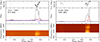 |
Fig. 1. Observed profiles and its variations in each sub-band of the MeerKAT dataset, after applying the Faraday rotation correction based on the obtained RMs in Table 2. The right panel refers to the L band and the left to the UHF band. In both panels, the black, red, and blue lines are the total intensity, linear, and circular polarization, respectively. |
Although the MeerKAT data are far more precise than those of Parkes, parameters such as proper motion and the orbital period derivative, Ṗb, require a longer timing baseline. Therefore, the data gathered by the Parkes telescope are included our timing analysis to complement the precise but short MeerKAT dataset.
3. Data analysis
3.1. Interstellar magnetic gield
Faraday rotation, which describes the rotation of the polarization angle along the LOS when a magnetic field in the same direction is present, was seen in the MeerKAT data. This is characterized by the rotation measure (RM). With the RM and DM, the average magnetic field in the direction of the LOS can be calculated based on the equation,
 (4)
(4)
The inferred ⟨B∥⟩ is listed in Table 2. To determine these values, we used the measured RM and DM, in Tables 2 and 3, respectively. The measured RM was also used to correct the Faraday rotation, and the resulting polarization angles are shown in the uppermost panels of Figure 1.
Our measurements of the rotation measure (RM), and the corresponding average magnetic field along the LOS.
Mean values and the nominal 1σ uncertainties of the best-fit with the obtained EFAC, EQUAD, DM noise, and red noise from the timing analysis and the comparison with LO06.
3.2. Timing analysis
Pulsar timing models every rotation of the pulsar using the times of arrival (ToAs) of the observed pulses at the telescope and thereby obtains measurements of spin, orbital, and astrometric parameters. These ToAs are generated by cross-correlating the pulse profile of an observation with a reference template, traditionally constructed by adding several of the brightest observations for a particular observing band before smoothing. Due to the intrinsic profile variations in PSR J1439−5501, we generated templates to account for the individual profiles at each sub-band. For the Parkes data, separate templates were created for each combination of front-end and back-end due to the different bandwidths, centre frequencies, and frequency resolution.
The timing analysis was done using the TEMPO2 software (Hobbs et al. 2006), and the Bayesian extension TEMPONEST (Lentati et al. 2014). We used the Solar System ephemeris, DE440 (Park et al. 2021), with the timing standard, International Atomic Time (TAI). To compensate for the timing offsets between telescopes and backends, a time offset (known as a JUMP) was fitted between each dataset using the MeerKAT L-band data as a reference. Using the results from TEMPO2, the noise properties and the posterior distributions of the timing parameters were investigated by using TEMPONEST (Section 3.3).
Due to the low eccentricity of the system, we use the Laplace-Langrange parameters, which are implemented in the ELL1 orbital model (Lange et al. 2001) instead of the orbital eccentricity (e), longitude of periastron (ω) and time of passage through periastron (T0) used for eccentric orbits:
 (5)
(5)
The reason for this is that, for low-eccentricity orbits, ω and T0 have an extremely high correlation, while Tasc, η and κ are well-defined for orbits with an arbitrarily small eccentricity. The latter can be derived as:
 (6)
(6)
The Shapiro delay is usually quantified with two PK parameters: range (r) and shape (s). In GR, these relate to the companion mass (mc) and orbital inclination (i) as follow (Damour & Taylor 1992):
 (7)
(7)
where  s is an exact quantity, the solar mass parameter (
 , Prša et al. 2016) in time units.
The problem with this description is that, apart from orbital inclinations close to 90°, these parameters are highly correlated. The ELL1H model gets around this problem by describing the Shapiro delay using the same harmonic approach used by the ELL1 model to describe the geometric delay with low-eccentricity orbits: its PK parameters, h3 and h4, describe the amplitude of the third and fourth orbital harmonics of the Shapiro delay. In GR, these are given by:
 (8)
(8)
where ς is the ‘orthometric ratio’, which like s depends only on i:
 (9)
(9)
In the case of moderately high inclinations, where harmonics above the fourth become detectable, h3 and h4 have a correlation of 0.5; in that limit h3 and ς provide a better description of the Shapiro delay. We use the latter parameters to describe the Shapiro delay of PSR J1439−5501.
3.3. Noise analysis
The TEMPONEST software was used to analyze the noise in pulsar timing based on the Bayesian statistics. The noise is broken down into types: white-noise, red-noise (where the variations at long time scales are larger than those at short time scale, RN), and DM noise. As the Shapiro delay is expected to give a residual of only ∼10 μs, high S/N observations in combination with full noise modelling is required.
The white-noise is described by the EFAC and EQUAD parameters. EFACs are a simple multiplier applied to the ToA uncertainties, used to weight the different observing modes (Hobbs et al. 2006). In contrast, EQUAD describes a separate source of white noise that is added in quadrature. The resulting uncertainties, including EFAC and EQUAD, are given by
 (10)
(10)
where αi is the original uncertainty, σi is EFAC, and βi is EQUAD, respectively. The EFAC and EQUAD have been applied to the Parkes, MeerKAT L and UHF bands, separately.
The frequency-dependent delay of the pulse due to the IISM is measured as the DM. Its variations over time, due to the relative motion of the pulsar system, Solar System, and the interstellar medium, cause delays and advances in the timing of the pulsar. This can be measured and removed when broad bandwidth observations are available. DM variations are usually a red noise process which TEMPONEST describes as a power-law (Lentati et al. 2014).
The spin noise of a pulsar is the major cause of frequency-independent red-noise. As with the DM noise, this is fit using a power law.
All the resulting noise parameters, obtained from TEMPONEST, and the pulsar parameters are fit using the noise models listed in Table 3. Figure 2 shows the post-fit residuals with a corresponding reduced-χ2, closed to unity.
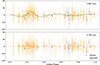 |
Fig. 2. Noise-free residuals in terms of the orbital phase. The level of uncertainties above 15 μs are dimmed in order to describe the trend clearly. The RMS levels are displayed in the upper right corner of each plot. Top: post-fit residuals with fixed h3 = 0, and η = 1. Notice that some of the Shapiro delay signature is absorbed by Keplerian orbital parameters. However, the Shapiro delay is still prominent. Lower: Post-fit residuals with the best-fit parameters in Table 3. Timing jumps have been applied to each receiver to account for any time offset. The size of the error-bars have been scaled with the corresponding EFAC and EQUAD. |
Figure 2 shows a clear signature of the Shapiro delay which cannot be fully absorbed into the other orbital parameters. By fitting for h3 and ς the structure is completely removed; also, h3 and ς are not covariant with any other parameters. There is a degree of covariance between h3 and ς, but the Shapiro delay is measurable with high significance.
4. Discussion
4.1. Mass and inclination
The two measured Shapiro delay parameters, h3 and ς, are plotted in the mass–mass diagram (Figure 3) and can be used to determine the masses and inclination of the system. The posterior of the relation between h3 and ς from TEMPONEST was transformed into the cos i − Mc and into the Mp − Mc spaces to illustrate the 2D Bayesian probability distribution functions (PDFs). The 2D PDF was marginalised to show 1D PDFs of the mass and the inclination. The 34.1% of the PDF on either side of the mean is plotted and provides the 1σ-equivalent uncertainty levels.
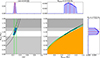 |
Fig. 3. Mass–mass diagram and the marginalised histograms. The black and green solid lines indicate 1σ range of h3 and ς, respectively. The companion mass, the inclination angle as well as the pulsar mass were determined based on the probability density distribution (PDF). The measured values (solid red lines), and uncertainties (dashed red lines) are determined from the median, and 68.1% confidence intervals, respectively. However, the error scale of the pulsar mass is large because of the shallow angle between the h3 and ς curves. The red point indicates the peak position of the posterior distributions of the measured masses from TEMPONEST. The parts of a tail, exceeding the Chandrasekhar mass (Mch = 1.48 M⊙) which is shown as a dark grey, were truncated. We also excluded the PDFs below the minimum neutron star mass, Mpulsar, min = 1.17 M⊙, determined by Suwa et al. (2018). The light grey is the outside of the range of the expected companion mass by PA13. |
The determined inclination angle and the masses without any additional constraints are  ,
,  M⊙, and
  M⊙, respectively. Although the NS and WD mass limits from the Shapiro delay and other timing and scintillation parameters are not very constraining (see Section 4.5), we can infer a better pulsar mass limit by assuming that the white dwarf does not exceed the Chandrasekhar mass limit, Mch = 1.48 M⊙ (Yoon & Langer 2004), and by assuming that the pulsar is heavier than the lightest ever discovered (Mns > 1.17 M⊙). Suwa et al. (2018) showed that the expected minimum mass of a pulsar from core-collapse supernova explosion is 1.17 M⊙. Therefore, we used such mass limits as priors, which truncated the PDFs, and the nature of WD and NS allowed the derivation of narrower constraints on the masses.
The probability density distribution suggests that the inclination angle is i = 75(1)°. This is consistent with what was constrained in PA13, namely, i ≥ 55°, assuming the Chandrasekhar-mass limit for the white dwarf. The derived mass of the companion,  M⊙, is also consistent with PA13: 1.0 ≲ Mc/M⊙ ≲ 1.3. We note that the upper uncertainty is not as significant, as it appears as a consequence of the truncation of the tail above the Chandrasekhar-mass limit. The pulsar mass from our analysis (
 ) is also compatible with the value from PA13 (Mp ≲ 2.2 M⊙). The measurements are summarised in Table 3.
McKee et al. (2020) showed that the distribution of the masses of pulsar WD companions is largely bimodal. One group consists of pulsar-He WD systems, with measured masses up to 0.4 M⊙, where the WD mass is closely tied to the orbital period (Tauris & Savonije 1999), a second group consists of slower MSPs with companion masses between 0.7 and 0.9 M⊙. There were then two outliers, one of them being PSR J2222−0137 (Guo et al. 2021), which has a companion mass of 1.319(4) M⊙.
Recently, in their study of PSR J1528−3146, Berthereau et al. (2023) noted that the latter’s companion mass ( ) is similar to that of PSR J2222−0137 and, thus, so are its spin and orbital properties; this suggests that these systems have a common evolutionary history and also that their companion masses may form a third discrete group. The spin properties and orbital characteristics of PSR J1439−5501 are similar to those of the two aforementioned binaries, and its companion mass, although not as precisely measured, is also consistent with the existence of a 1.3-M⊙ group. Finally, precise measurements of these WD masses (and of the distance to these systems) would allow for an improvement of their cooling age and perhaps even an opportunity to test the WD cooling models used by PA13.
The uncertainties in our measurements show that there is a significant improvement in the determined pulsar mass and geometry compared to PA13. However, the uncertainty in Mp remains relatively large because (despite the low correlation between the h3 and ς parameters and their relatively precise measurements) the constraints they introduce in the Mc − cos i and especially in the Mc − Mp space intersect at shallow angles; this is the ultimate reason why it is generally difficult to obtain precise masses based solely on the Shapiro delay, even with precise estimates of ς and h3 (Freire & Wex 2010).
The measurement of additional PK parameters like  would be useful to constrain the precise masses, but it is difficult in this case given the very low eccentricity of the orbit. For this reason, the orbital period derivative, Ṗb, is the PK parameter most likely to be detected next. To forecast the detection of Ṗb we must first estimate the distance.
4.2. Timing parallax limit
PA13 limited the distance to PSR J1439−5501 using optical data of the companion in combination with WD-cooling models. If the companion is a CO-WD, the distance range is 710 pc ≲ d ≲ 1200 pc. In contrast, supposing an ONe-WD results at the distance of 650 pc ≲ d ≲ 1200 pc, with the smaller distances corresponding to more massive WDs.
We used PyGEDM (Price et al. 2021) to calculate the distance with the Galactic electron density distribution models, YMW16 (Yao et al. 2017) and NE2001 (Cordes & Lazio 2002). The distances (and parallaxes) are 655 pc (1.53 mas) and 604 pc (1.66 mas), respectively, as listed in Table 4. We adopted the typically used 20% uncertainty level (e.g. Cordes & Lazio 2003; Straal et al. 2020). However, the exact uncertainty for individual sources is difficult to estimate. Shamohammadi et al. (in prep.) showed that the distance determined by the Galactic electron density distribution models is highly unreliable. Therefore, interpreting the physical quantities depending on the distance in this paper requires caution. Using this same uncertainty they are also consistent with the near end of the estimates in both WD models of PA13.
4.3. Forecast for Ṗb
To predict when it will be possible to detect Ṗb, we generated mock ToAs using the pulsar ephemeris (Figure 4) by applying the ‘fake’ plugin, supported by TEMPO2 (Hobbs et al. 2006). The ToAs were then analyzed by using LIBSTEMPO (Vallisneri 2020), a Python wrapper for TEMPO2. Several assumptions were made for the simulation. First, there will be observations every 3 months but with a randomness in the precise date of 30% of the observation interval. As well as being more realistic, such randomness can help avoiding sampling issues. Second, we considered the planned upgrades of MeerKAT. We largely followed the same description as in Hu et al. (2020) with the SKA mid-frequency array beginning in 2027 and the MeerKAT extension prior to this (however using the revised date of 2024 rather than 2022). We use the same radiometer noise levels for each phase as determined in Hu et al. (2020) and calculated the expected improvement based on our current dataset which has a root-mean-squared (RMS) residual of 4.3 μs. The anticipated radiometric error, calculated from the collecting area between MeerKAT and each phase, for the simulated ToAs in each phase is listed in Table 5. Third, we used the DM distance obtained in Section 4.2 to calculate the orbital period change.
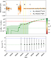 |
Fig. 4. Timing residuals of the simulated datasets, with, and without Ṗb, which are Model 1 (blue) and Model 2 (orange), respectively, shown in the top panel. The middle panel illustrates the difference in the log-likelihood between two models with respect to the time in a MJD scale. The red-dotted lines indicate the significance of detection (≥3σ), either from fitting and from lnL. The color bar scale indicates the significance of the fitting of Ṗb. The detection is expected to be around 64 000–65 000 MJD. The lower panel indicates the expected measurements on Ṗ effect over time. The expected value and the 3σ uncertainty range of Ṗb are depicted with green and blue dotted lines, separately. |
In the simulation, the expected Ṗb was included in our timing model while keeping the other parameters as measured2. To calculate the Ṗb there are several contributions caused by different physical effects (Lorimer & Kramer 2004),
 (11)
(11)
The first term is the intrinsic gravitational wave damping as predicted by general relativity, given by,
 (12)
(12)
The expected  is
is  .
.
The second effect is the Shklovskii effect (Shklovskii 1970) that occurs due to the changing orientation with respect to the LOS as the pulsar moves, and so is dependent on proper motion and distance:
 (13)
(13)
Given the measured proper motion and estimated distance using YMW16 model, the expected Shklovskii effect is  . The uncertainty is determined by assuming a 20% uncertainty in DM distance, which is equivalent to the DM distance error calculated from NE2001 (Straal et al. 2020). We also applied this relative uncertainty to the YMW16 model.
The contribution from Galactic acceleration must also be considered. We used the parameters as in Guo et al. (2021). Damour & Taylor (1991) discussed the effect, and later, Nice & Taylor (1995) improved the equation by including a flat rotation curve as follows:
 (14)
(14)
where β = (d/R⊙)cos b − cos l, kz(109 cm s−2)≃2.27zkpc + 3.68(1 − e−4.31zkpc) from Holmberg & Flynn (2004), R⊙ is the Galactocentric distance at the location of the Sun, and Ω⊙ = Θ⊙/R⊙ is the Galactic angular velocity of the Sun. Like in Guo et al. (2021), we calculated the Galactic acceleration using Equation (14) with the distance from the Sun to the Galactic centre, R⊙ = 8275(34) pc and with the Sun‘s Galactic circular velocity, Θ⊙ = 240.5 ± 4.1 km s−1, based on the measurements provided by the GRAVITY collaboration (Abuter et al. 2021). Accordingly, for PSR J1439−5501 the orbital period change by Galactic acceleration is expected to be  . As with the Shklovskii contribution, we considered 20% uncertainty of the DM distance to find the error of
  . For this system, this effect is about 100 times smaller than
  , so it will not be considered further.
The total expected orbital period change of  by summing all the effects. We used this value to produce the mock data points in order to forecast the detection of the orbital period derivative.
In order to measure the contribution of Ṗb two models were compared, model one,  ), includes the intrinsic Ṗb effects, while model two,
  ), only contains the extrinsic orbital period change. In all cases, we considered only white noise, since the long-term red-noise properties are not well-known. This is a simple way to forecast the parameter detection but also has a limitation in that strong red-noise may limit timing accuracy. Both models contain the timing parameters in Table 3. Here, D is the timing residuals and P is the given timing parameters.
Summary of RMS-levels for the simulated datasets.
We considered a likelihood function to check the performance of each model. The function is given by:
 (15)
(15)
where xi is the post-fit timing residuals, and σi is the size of uncertainties of the individual ToAs, respectively. In the simulation, we used a log-likelihood function, lnL, where a higher value indicates a better fit. The difference between the likelihoods of two models is described by:
 (16)
(16)
Figure 4 shows that the model,  ), progressively becomes better as the timing-baseline increases. However, only a single realization (green-solid line in Figure 4) is ambiguous for forecasting in the low S/N regime so we considered 80 realizations and have plotted the mean and standard deviation at each epoch. All timing parameters were fitted with LIBSTEMPO at each step. Around December 2036, the significance of the Ṗb starts exceeding the 3-σ level.
If the Shklovskii effect cannot be determined more precisely, the gravitational damping effect cannot be measured with better than 2-σ significance. To constrain the gravitational damping, a reliable distance measurement is essential. Given the small distance to the system (0.6–0.7 kpc), it is likely that VLBI distance measurements (Ding et al. 2023) will be able to significantly improve the distance measurement, and therefore improve the estimate of  and
and  . Because of interstellar scintillation, the pulsar’s flux varies between 0.2 and 1.5 mJy but its 10% duty cycle would assist with a VLBI parallax. Unfortunately, the current VLBI cannot detect the source due to its location in the far south. Therefore, a southern hemisphere network is required to find the parallax.
Another potential application of the orbital period change in PSR J1439−5501 is testing gravity theories. This was done using the intrinsic orbital period derivative estimated for PSR J2222−0137 (Guo et al. 2021), which matches closely the GR prediction for  ; the difference is so small that it introduces a tight constraint on the emission of dipolar gravitational waves (DGW), a prediction of many alternative theories of gravity (Eardley 1975; Damour & Esposito-Farese 1993). This constraint is especially relevant because the mass of PSR J2222−0137 is within a range from 1.6 ∼ 1.9 M⊙ (Shibata et al. 2014; Shao et al. 2017), where DGW emission could be strongly amplified by the spontaneous scalarisation of neutron stars, a non-perturbative effect that can occur in some gravity theories, like the scalar-tensor theories of Damour & Esposito-Farese (1993). The non-detection of DGW emission in PSR J2222−0137 greatly constrained the occurrence of this phenomenon (Zhao et al. 2022). However, it is important to emphasize once again that in order to effectively test gravity theories, the distance needs to be precisely measured.
Whether PSR J1439−5501 can be used for a similar experiment or not will depend on its exact mass: if it is inside the aforementioned mass range (something allowed by the current uncertainty region), then it might provide limits on scalar-tensor theories of gravity that are similar to, or (if a precise VLBI estimate is available) better than those provided by PSR J2222−0137, the reason for this is the unusually small predicted sum of Galactic accelerations.
4.4. Characteristic age
As in the case of the binary orbital derivative, the observed spin derivative is also affected by Shklovskii effect and Galactic acceleration. By replacing Pb in Equations (13) and (14), the extrinsic spin change can be determined. Assuming the identical distance setting and Galactic model used in the previous section, the rate of spin change from the Shklovskii effect and Galactic acceleration are,  , respectively. Therefore, the intrinsic spin variation is
  .
.
Based on the corrected spin variation, the characteristic age is updated here. Assuming that the braking index n = 3, the spin-down age is expressed as:
![Mathematical equation: $$ \begin{aligned} \tau _{\rm c} = \frac{P}{ (n - 1) \dot{P} } \left[ 1 - \left( \frac{P_0}{P} \right)^{n-1} \right] \sim \frac{P}{2 \dot{P}}, \end{aligned} $$](/articles/aa/full_html/2024/09/aa47505-23/aa47505-23-eq47.gif) (17)
(17)
where P0 is the initial spin period and the second expression assumes that the braking index n is 3 and that P0 ≪ P, which is generally not true for recycled pulsars. LO06 derived τc = 3.2 Gyr based only on the observed Ṗ, while Kiziltan & Thorsett (2010) derived τc = 4.46 Gyr for PSR J1439−5501 by assuming a heliocentric transverse velocity (v⊥) of 100 km/s. Our measurement of the proper motion allows fora determination of v⊥ = μd = 22 ± 4 km s−1, and an estimate of the bias on Ṗ, resulting in the spin-down age, 3.0930 3) Gyr, which agrees with the LO06 estimate given the small transverse velocity.
As discussed by PA13, these τc estimates are significantly larger than the cooling age of the companion WD (between 0.1 and 0.2 Gyr for a CO WD companion, and 0.1 and 0.4 Gyr for ONeMg WD companion); as they pointed out, the likely reason for this apparent discrepancy is the assumption that P0 ≪ P, which (as noted above) is unlikely to be true for recycled pulsars. This means that although τc generally provides a useful upper limit on the age of recycled pulsars, it can be a significant over-estimate.
As discussed by Tauris et al. (2012), for systems with massive companions like PSR J1439−5501, the accretion phase was short-lived. Thus, the amount of angular momentum transferred to the pulsar was small, which is consistent with a post-recycling spin period similar to what we observe now. This also suggests that the pulsar mass has changed very little during recycling (Cognard et al. 2017). Thus, our measurement of the pulsar mass represents a neutron star birth mass.
4.5. Scintillation analysis
The observations with MeerKAT show clear evidence of scintillation. In this section, we describe an analysis of the observed scintillation to constrain the relative motion and the orbital geometry of PSR J1439−5501.
We investigated the scintillation arcs, shown in Figure 5, at each epoch from August 2020 to May 2022. In observations separated by roughly a day (e.g. MJDs 59419–59420), the arcs were clearly flipped along the fD axis, which occurs when the effective velocity changes in its direction, as discussed in (Rickett et al. 2014). To take account of this effect, we took the sign of the effective velocity based on the direction of the power asymmetry. From each observation, we formulated ‘normalized secondary spectra’ as in Reardon et al. (2020), with the map parabolae of different curvatures to vertical lines. Summing over τ, this results in a power profile of S(η). To estimate the uncertainty of the arc curvatures, we took the measured full width at half maximum of this Gaussian divided by the S/N in the S(η) space.
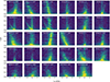 |
Fig. 5. Secondary spectra showing scintillation arcs. On the top of each plot, the corresponding MJD and observing frequencies are indicated. The red-dotted line delineates the best-fit curvature of the arc. The pulsar scintillates in the UHF band strongly, thus, the arcs have broader widths than in the L band. The arc curvatures at 59515.6 and at 50520.5 are notably steep, which suggest that the effective velocity is small, while the ones at 59466.3 and at 59718.8 are not prominent. |
The interference between two signals arriving at angle θ has a fringe rate of ft = veff(θ2 − θ1)/λs and delay of  . The secondary spectrum (the 2D power spectrum of scintillation) expresses the power as a function of fD and τ, being Fourier conjugate variables of t and ν. Due to their common dependence on θ, these parameters are related as
  , where
  – a collection of images results in a parabolic distribution of power, where η is the arc curvature. As in Mall et al. (2022), we chose to work with
 (18)
(18)
as it does not diverge when veff, || → 0.
By adding a factor on the size of the errors, EFAC, as in timing, we adjusted the size of the error scales of the arcs. Including an EFAC is also beneficial in accounting for some potential systematic errors, likely caused by the power asymmetries of the scintillation arcs; these can arise from local phase gradients across the screen, and will shift the apex of the scintillation arc in fD and τ. The EFAC used here is 3.867.
We found that the measured arc curvatures show a clear orbital modulation and a weak annual variation as shown in Figure 6. The arcs, expressed in Equation (18), were further analysed to investigate the relative motion of the Earth, the pulsar, and the screen via an Markov chain Monte Carlo (MCMC) posterior sampling, as in Mall et al. (2022), with an anisotropic model by using scintools3 (Reardon et al. 2020). The measured proper motion and orbital inclination in Table 3 were given as the priors for the MCMC sampling. However, the inclination angle is degenerate, with two possible solutions. Consequently, we considered two models, one with i = 75(1)° (case A) and another with i = 105(1)° (case B). Both models show the similar χ2, thus, it is still an open question whether the inclination is the first case, or the second one. We omitted a prior for the distance because the distance is not well determined.
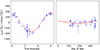 |
Fig. 6. Orbital (left) and the annual effect (right) of the measured arc curvatures. The orbital modulation is evident, while the annual variation is weak since the binary has shorter orbital period than the Earth. The insignificant annual variation leads to the large errors on ψ − s. The data points around veff = 0 show very steep arc curvatures in Figure 5. |
Table 6 summarises the results from the MCMC sampling, and the corresponding posteriors are shown in Figure A.1. Both cases are consistent with each other, except for Ω which differs depending on the initial value of i. The measured distance is 0.44(15) kpc, and 0.45(16) kpc, for the case A, and B, respectively. This is 1-σ consistent with the DM derived distances in Section 4.2 and the distance in PA13. The determined fractional distances by the corresponding models are 0.42(8) for all cases, suggesting that the screen is closer to the pulsar than the Earth.
Parameters and the results determined through scintillation curvature analysis.
The results of the MCMC sampling suggest that the screen is 260 ± 100 pc away from the Earth. The screen distance is possibly coincident with the Local Bubble boundary, discussed in McKee et al. (2022) but we will need a more precise screen distance to make this association.
However, the entire results based on the MCMC sampling should be treated with caution as there are significant correlations between the parameters (Table 6). Commonly, C(d, vIISM), C(d, sfrac), C(ψ, Ω), and C(sfrac, vIISM) show a significant covariance in both models. Although we detect a clear orbital variation, the annual variation is poorly constrained. Phase gradients across the scattering screen arise from spatial gradients in DM. This results in tilted autocorrelation functions (Reardon & Coles 2023), or equivalently in parabolic arcs with their focus offset from the origin. We see evidence of this from our asymmetric arcs, but not sufficient S/N to measure this in every epoch; for our purposes, this would introduce systematic biases in our measurements of the arc curvatures. Thus, more precise accounting of the phase gradients, better annual coverage, and an independent distance measurement will allow us to more tightly constrain these results.
5. Conclusion and summary
We combined three years of data from MeerKAT and five years from Parkes in order to measure a Shapiro delay in PSR J1439−5501. Due to significant profile variations with frequency we retained frequency resolution in the data and used frequency dependent templates to determine the ToAs. These ToAs were analyzed with TEMPO2 and TEMPONEST (which also modelled the white noise, DM noise, and timing noise). Due to the low eccentricity and relatively high inclination of the system, the ELL1H model was used. We measured the orthometric amplitude of the Shapiro delay to be 2.9(2) μs and the orthometric ratio 0.75(3). Additionally, we detected the proper motion for the first time, 7.02(9) mas yr−1.
Based on the Shapiro delay, we measured the mass of PSR J1439−5501 to be  M⊙, the mass of the companion to be
  M⊙, and the orbital inclination angle to be 75(1)°. The spin, orbital and mass properties imply a system similar to PSR J2222−0137 (Guo et al. 2021) and PSR J1528−3146 (Berthereau et al. 2023), this is further corroborated by the masses of the WDs in these systems, all of which are consistent with 1.3 M⊙. This mass measurement confirms the trend seen by McKee et al. (2020), where the massive WDs around pulsars are seen to belong to three groups with a narrow mass distribution.
The distance could not be constrained by parallax through pulsar timing. Thus, we estimated it based on the YMW16 and the NE2001 models and compared it to the estimate via optical observations of the companion. If we use our estimate for the companion WD mass in Fig. 3 from PA13, we obtain distances smaller than 800 pc, these are consistent with the DM distance estimates that suggest that the system is at about 0.66 kpc from the Sun. Future VLBI observations of this system would likely determine the distance precisely, especially if the estimate from the DM model (or even better, if the smaller distance estimate from scintillation below) is correct.
The relatively large uncertainty of the pulsar mass is due to the intrinsic difficulty of measuring masses using the Shapiro delay only, especially for systems where the orbits are not close to edge-on. Improvements in the measurement of the Shapiro delay in the future will help improve these mass measurements; however, it improves slowly with time. A precise estimate of  would result in more precise mass estimates than those obtained from the Shapiro delay, but this will also be difficult: our simulations suggest that continued MeerKAT observations of PSR J1439−5501 will be able to detect
  within few decades, but improving its measurement will be limited by the uncertainty on the Shklovskii effect. A precise VLBI distance and resulting estimates of
  – or, alternatively, from scintillation studies – will eventually be important for a precise estimate of
  and the masses of the components.
Improved masses would be useful for several reasons: an improved WD mass could help confirm the third group in WD mass observed by McKee et al. (2020), and help determine how narrow the WD mass distribution is within the 1.3-M⊙. Precise measurements of these WD masses – and of the distance to these systems – will, together with the existing optical data, allow for improved estimates of their cooling ages and, perhaps, even test massive WD cooling models. Regarding the pulsar masses, as discussed by Cognard et al. (2017), in all of these systems, there was a very small amount of mass transfer; this means that we’re measuring neutron star birth masses. Knowing the latter’s distribution is important for understanding the physics of supernovae. Furthermore, if the mass of the pulsar can be constrained precisely from Shapiro delay and is within the mass gap of spontaneous scalarisation, then a precise Ṗb measurement would be useful for constraining alternative theories of gravity (Zhao et al. 2022).
Finally, we studied the scintillation patterns observed in PSR J1439−5501. We noticed that the orbital modulation is stronger than the annual variation. Results from MCMC sampling suggest that the fractional screen distance is positioned at sfrac = 0.42(8), closer to the pulsar than the Earth. The screen distance of 260 ± 100 pc is potentially connected to the edge of the Local Bubble, as has been suggested in McKee et al. (2022). However, due to significant correlations within the MCMC modelling, the measurements of the orbit via scintillation are currently limited. The scintillation distance is 1-σ consistent with estimate of the YMW16 model as well as with the optical results by PA13. Systematic errors come from a physical effect, namely, the phase gradients, which cause asymmetries in scintillation arcs and are not currently modeled in our analysis. A proper modelling of these, as well as more complete annual coverage, in addition to a more precise distance determination, will help constrain the obtained parameters and the 3D motion of PSR J1439−5501. As discussed above, these advances would also improve the estimates of  and
and  .
.
This is calculated by using the MCMC-based code https://github.com/astrophysics91/PBDOT-calculator
Acknowledgments
The MeerKAT telescope is operated by the South African Radio Astronomy Observatory, which is a facility of the National Research Foundation, an agency of the Department of Science and Innovation. SARAO acknowledges the ongoing advice and calibration of GPS systems by the National Metrology Institute of South Africa (NMISA) and the time space reference systems department of the Paris Observatory. MeerTime data is housed on the OzSTAR supercomputer at Swinburne University of Technology supported by ADACS and the Gravitational Wave Data Centre via Astronomy Australia Ltd. We appreciate to Dr. Norbert Wex (MPIfR), and Dr. Gregory Desvignes (MPIfR) to provide discussions about the change of the binary orbital phase. We also thank to Dr. Nataliya Porayko (University of Milano-Bicocca). She supported software installation and instruction.
References
- Abuter, R., Amorim, A., Bauböck, M., et al. 2021, A&A, 647, A59 [NASA ADS] [CrossRef] [EDP Sciences] [Google Scholar]
- Arzoumanian, Z., Brazier, A., Burke-Spolaor, S., et al. 2018, ApJS, 235, 37 [CrossRef] [Google Scholar]
- Bailes, M., Barr, E., Bhat, N. D. R., et al. 2018, Proceedings of MeerKAT Science: On the Pathway to the SKA (MeerKAT2016), online at https://pos.sissa.it/cgi-bin/reader/conf.cgi?confid=277, 11 [Google Scholar]
- Berthereau, A., Guillemot, L., Freire, P. C. C., et al. 2023, A&A, 674, A71 [NASA ADS] [CrossRef] [EDP Sciences] [Google Scholar]
- Cognard, I., Freire, P. C. C., Guillemot, L., et al. 2017, ApJ, 844, 128 [NASA ADS] [CrossRef] [Google Scholar]
- Cordes, J. M., & Lazio, T. J. W. 2002, ArXiv e-prints [arXiv:astro-ph/0207156] [Google Scholar]
- Cordes, J. M., & Lazio, T. J. W. 2003, ArXiv e-prints [arXiv:astro-ph/0207156] [Google Scholar]
- Cordes, J. M., Rickett, B. J., Stinebring, D. R., & Coles, W. A. 2006, ApJ, 637, 346 [NASA ADS] [CrossRef] [Google Scholar]
- Damour, T., & Deruelle, N. 1986, Ann. Inst. Henri Poincaré Phys. Théor, 44, 263 [Google Scholar]
- Damour, T., & Taylor, J. H. 1991, ApJ, 366, 501 [NASA ADS] [CrossRef] [Google Scholar]
- Damour, T., & Taylor, J. H. 1992, Phys. Rev. D, 45, 1840 [NASA ADS] [CrossRef] [Google Scholar]
- Damour, T., & Esposito-Farese, G. 1993, Phys. Rev. Lett., 70, 2220 [NASA ADS] [CrossRef] [Google Scholar]
- Ding, H., Deller, A. T., Stappers, B. W., et al. 2023, MNRAS, 519, 4982 [NASA ADS] [CrossRef] [Google Scholar]
- Eardley, D. M. 1975, ApJ, 196, L59 [NASA ADS] [CrossRef] [Google Scholar]
- Faulkner, A. J., Stairs, I. H., Kramer, M., et al. 2004, MNRAS, 355, 147 [Google Scholar]
- Ferdman, R. D., Stairs, I. H., Kramer, M., et al. 2010, ApJ, 711, 764 [NASA ADS] [CrossRef] [Google Scholar]
- Fonseca, E., Cromartie, H. T., Pennucci, T. T., et al. 2021, ApJ, 915, L12 [NASA ADS] [CrossRef] [Google Scholar]
- Freire, P. C. C., & Wex, N. 2010, MNRAS, 409, 199 [NASA ADS] [CrossRef] [Google Scholar]
- Geyer, M., Krishnan, V. V., Freire, P. C. C., et al. 2023, A&A, 674, A169 [NASA ADS] [CrossRef] [EDP Sciences] [Google Scholar]
- Guo, Y. J., Freire, P. C. C., Guillemot, L., et al. 2021, A&A, 654, A16 [NASA ADS] [CrossRef] [EDP Sciences] [Google Scholar]
- Hobbs, G. B., Edwards, R. T., & Manchester, R. N. 2006, MNRAS, 369, 655 [Google Scholar]
- Holmberg, J., & Flynn, C. 2004, MNRAS, 352, 440 [NASA ADS] [CrossRef] [Google Scholar]
- Hu, H., Kramer, M., Wex, N., Champion, D. J., & Kehl, M. S. 2020, MNRAS, 497, 3118 [NASA ADS] [CrossRef] [Google Scholar]
- Kiziltan, B., & Thorsett, S. E. 2010, ApJ, 715, 335 [Google Scholar]
- Kramer, M., Stairs, I. H., Venkatraman Krishnan, V., et al. 2021, MNRAS, 504, 2094 [CrossRef] [Google Scholar]
- Lange, C., Camilo, F., Wex, N., et al. 2001, MNRAS, 326, 274 [NASA ADS] [CrossRef] [Google Scholar]
- Lentati, L., Alexander, P., Hobson, M. P., et al. 2014, MNRAS, 437, 3004 [NASA ADS] [CrossRef] [Google Scholar]
- Lorimer, D. R., Faulkner, A. J., Lyne, A. G., et al. 2006, MNRAS, 372, 777 [NASA ADS] [CrossRef] [Google Scholar]
- Lorimer, D. R., & Kramer, M. 2004, Handbook of Pulsar Astronomy (Cambridge: Cambridge University Press), 4 [Google Scholar]
- Main, R. A., Sanidas, S. A., Antoniadis, J., et al. 2020, MNRAS, 499, 1468 [NASA ADS] [CrossRef] [Google Scholar]
- Mall, G., Main, R. A., Antoniadis, J., et al. 2022, MNRAS, 511, 1104 [CrossRef] [Google Scholar]
- Manchester, R. N., Lyne, A. G., Camilo, F., et al. 2001, MNRAS, 328, 17 [NASA ADS] [CrossRef] [Google Scholar]
- Manchester, R. N., Hobbs, G. B., Teoh, A., & Hobbs, M. 2005, AJ, 129, 1993 [Google Scholar]
- McKee, J. W., Freire, P. C. C., Berezina, M., et al. 2020, MNRAS, 499, 4082 [NASA ADS] [CrossRef] [Google Scholar]
- McKee, J. W., Zhu, H., Stinebring, D. R., & Cordes, J. M. 2022, ApJ, 927, 99 [NASA ADS] [CrossRef] [Google Scholar]
- Nice, D. J., & Taylor, J. H. 1995, ApJ, 441, 429 [NASA ADS] [CrossRef] [Google Scholar]
- Pallanca, C., Lanzoni, B., Dalessandro, E., et al. 2013, ApJ, 773, 127 [NASA ADS] [CrossRef] [Google Scholar]
- Park, R. S., Folkner, W. M., Williams, J. G., & Boggs, D. H. 2021, AJ, 161, 105 [NASA ADS] [CrossRef] [Google Scholar]
- Price, D. C., Flynn, C., & Deller, A. 2021, PASA, 38 [CrossRef] [Google Scholar]
- Prša, A., Harmanec, P., Torres, G., et al. 2016, AJ, 152, 41 [Google Scholar]
- Reardon, D. J., & Coles, W. A. 2023, MNRAS, 521, 6392 [NASA ADS] [CrossRef] [Google Scholar]
- Reardon, D. J., Coles, W. A., Bailes, M., et al. 2020, ApJ, 904, 104 [NASA ADS] [CrossRef] [Google Scholar]
- Rickett, B. J., Coles, W. A., Nava, C. F., et al. 2014, ApJ, 787, 161 [NASA ADS] [CrossRef] [Google Scholar]
- Shamohammadi, M., Bailes, M., Freire, P. C. C., et al. 2023, MNRAS, 520, 1789 [NASA ADS] [CrossRef] [Google Scholar]
- Shao, L., Sennett, N., Buonanno, A., Kramer, M., & Wex, N. 2017, Phys. Rev. X, 7, 041025 [Google Scholar]
- Shapiro, I. I. 1964, Phys. Rev. Lett., 13, 789 [Google Scholar]
- Shibata, M., Taniguchi, K., Okawa, H., & Buonanno, A. 2014, Phys. Rev. D, 89, 084005 [NASA ADS] [CrossRef] [Google Scholar]
- Shklovskii, I. S. 1970, Sov. Astron., 13, 562 [NASA ADS] [Google Scholar]
- Stinebring, D. R., McLaughlin, M. A., Cordes, J. M., et al. 2001, ApJ, 549, L97 [NASA ADS] [CrossRef] [Google Scholar]
- Straal, S. M., Connor, L., & van Leeuwen, J. 2020, A&A, 634, A105 [NASA ADS] [CrossRef] [EDP Sciences] [Google Scholar]
- Suwa, Y., Yoshida, T., Shibata, M., Umeda, H., & Takahashi, K. 2018, MNRAS, 481, 3305 [NASA ADS] [CrossRef] [Google Scholar]
- Tauris, T. M., & Savonije, G. J. 1999, A&A, 350, 928 [NASA ADS] [Google Scholar]
- Tauris, T. M., Langer, N., & Kramer, M. 2011, MNRAS, 416, 2130 [NASA ADS] [CrossRef] [Google Scholar]
- Tauris, T. M., Langer, N., & Kramer, M. 2012, MNRAS, 425, 1601 [NASA ADS] [CrossRef] [Google Scholar]
- Tauris, T. M., Kramer, M., Freire, P. C. C., et al. 2017, ApJ, 846, 170 [Google Scholar]
- Vallisneri, M. 2020, Astrophysics Source Code Library [record ascl:2002.017] [Google Scholar]
- van Straten, W., Demorest, P., & Osłowski, S. 2012, Astron. Res. Technol., 9, 237 [Google Scholar]
- Walker, M. A., Melrose, D. B., Stinebring, D. R., & Zhang, C. M. 2004, MNRAS, 354, 43 [NASA ADS] [CrossRef] [Google Scholar]
- Yao, J. M., Manchester, R. N., & Wang, N. 2017, ApJ, 835, 29 [NASA ADS] [CrossRef] [Google Scholar]
- Yoon, S. C., & Langer, N. 2004, A&A, 419, 623 [NASA ADS] [CrossRef] [EDP Sciences] [Google Scholar]
- Özel, F., & Freire, P. 2016, ARA&A, 54, 401 [Google Scholar]
- Zhao, J., Freire, P. C. C., Kramer, M., Shao, L., & Wex, N. 2022, Class. Quant. Grav., 39, 11LT01 [Google Scholar]
Appendix A: Posteriors
The posteriors obtained from TEMPONEST does not reflect physical distributions. Therefore, a conversion is required, expressed by
 (A.1)
(A.1)
where A is the central value, and B is the scaling factor, and i represents the raw posteriors. The related parameters are listed in Table A.1. Figure A.2 shows the posteriors, but with the scale before the conversion.
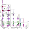 |
Fig. A.1. Posterior distributions of the case A (green with blue locator) and of the case B (violet with a red indicator). These posteriors result from the assumption that the screen is anisotropic. The longitude of the ascending node depends on the inclination angle, while most other parameters are consistent regardless of i. The posteriors of the proper motions were omitted since they are well determined without any significant correlations with other parameters. |
Summary of the timing parameters, the central values, and the scaling factors.
 |
Fig. A.2. Posteriors of the best-fit parameters. The proper motion and the coordinate, dispersion measurement and its variation, the epoch of periastron, and the orbital period are highly correlated. The Shapiro delay parameters are self-associated. They are also weakly linked with the projected semi-major axis. |
All Tables
Our measurements of the rotation measure (RM), and the corresponding average magnetic field along the LOS.
Mean values and the nominal 1σ uncertainties of the best-fit with the obtained EFAC, EQUAD, DM noise, and red noise from the timing analysis and the comparison with LO06.
Summary of the timing parameters, the central values, and the scaling factors.
All Figures
|
Fig. 1. Observed profiles and its variations in each sub-band of the MeerKAT dataset, after applying the Faraday rotation correction based on the obtained RMs in Table 2. The right panel refers to the L band and the left to the UHF band. In both panels, the black, red, and blue lines are the total intensity, linear, and circular polarization, respectively. |
| In the text | |
|
Fig. 2. Noise-free residuals in terms of the orbital phase. The level of uncertainties above 15 μs are dimmed in order to describe the trend clearly. The RMS levels are displayed in the upper right corner of each plot. Top: post-fit residuals with fixed h3 = 0, and η = 1. Notice that some of the Shapiro delay signature is absorbed by Keplerian orbital parameters. However, the Shapiro delay is still prominent. Lower: Post-fit residuals with the best-fit parameters in Table 3. Timing jumps have been applied to each receiver to account for any time offset. The size of the error-bars have been scaled with the corresponding EFAC and EQUAD. |
| In the text | |
|
Fig. 3. Mass–mass diagram and the marginalised histograms. The black and green solid lines indicate 1σ range of h3 and ς, respectively. The companion mass, the inclination angle as well as the pulsar mass were determined based on the probability density distribution (PDF). The measured values (solid red lines), and uncertainties (dashed red lines) are determined from the median, and 68.1% confidence intervals, respectively. However, the error scale of the pulsar mass is large because of the shallow angle between the h3 and ς curves. The red point indicates the peak position of the posterior distributions of the measured masses from TEMPONEST. The parts of a tail, exceeding the Chandrasekhar mass (Mch = 1.48 M⊙) which is shown as a dark grey, were truncated. We also excluded the PDFs below the minimum neutron star mass, Mpulsar, min = 1.17 M⊙, determined by Suwa et al. (2018). The light grey is the outside of the range of the expected companion mass by PA13. |
| In the text | |
|
Fig. 4. Timing residuals of the simulated datasets, with, and without Ṗb, which are Model 1 (blue) and Model 2 (orange), respectively, shown in the top panel. The middle panel illustrates the difference in the log-likelihood between two models with respect to the time in a MJD scale. The red-dotted lines indicate the significance of detection (≥3σ), either from fitting and from lnL. The color bar scale indicates the significance of the fitting of Ṗb. The detection is expected to be around 64 000–65 000 MJD. The lower panel indicates the expected measurements on Ṗ effect over time. The expected value and the 3σ uncertainty range of Ṗb are depicted with green and blue dotted lines, separately. |
| In the text | |
|
Fig. 5. Secondary spectra showing scintillation arcs. On the top of each plot, the corresponding MJD and observing frequencies are indicated. The red-dotted line delineates the best-fit curvature of the arc. The pulsar scintillates in the UHF band strongly, thus, the arcs have broader widths than in the L band. The arc curvatures at 59515.6 and at 50520.5 are notably steep, which suggest that the effective velocity is small, while the ones at 59466.3 and at 59718.8 are not prominent. |
| In the text | |
|
Fig. 6. Orbital (left) and the annual effect (right) of the measured arc curvatures. The orbital modulation is evident, while the annual variation is weak since the binary has shorter orbital period than the Earth. The insignificant annual variation leads to the large errors on ψ − s. The data points around veff = 0 show very steep arc curvatures in Figure 5. |
| In the text | |
|
Fig. A.1. Posterior distributions of the case A (green with blue locator) and of the case B (violet with a red indicator). These posteriors result from the assumption that the screen is anisotropic. The longitude of the ascending node depends on the inclination angle, while most other parameters are consistent regardless of i. The posteriors of the proper motions were omitted since they are well determined without any significant correlations with other parameters. |
| In the text | |
|
Fig. A.2. Posteriors of the best-fit parameters. The proper motion and the coordinate, dispersion measurement and its variation, the epoch of periastron, and the orbital period are highly correlated. The Shapiro delay parameters are self-associated. They are also weakly linked with the projected semi-major axis. |
| In the text | |
Current usage metrics show cumulative count of Article Views (full-text article views including HTML views, PDF and ePub downloads, according to the available data) and Abstracts Views on Vision4Press platform.
Data correspond to usage on the plateform after 2015. The current usage metrics is available 48-96 hours after online publication and is updated daily on week days.
Initial download of the metrics may take a while.