| Issue |
A&A
Volume 688, August 2024
|
|
|---|---|---|
| Article Number | A1 | |
| Number of page(s) | 11 | |
| Section | Galactic structure, stellar clusters and populations | |
| DOI | https://doi.org/10.1051/0004-6361/202450172 | |
| Published online | 30 July 2024 | |
Gaia DR3 detectability of unresolved binary systems
1
Leiden Observatory, Leiden University, Einsteinweg 55, 2333 CC Leiden, The Netherlands
e-mail: This email address is being protected from spambots. You need JavaScript enabled to view it.
2
School of Physics and Astronomy, Monash University, Clayton, VIC 3800, Australia
3
Centre of Excellence for Astrophysics in Three Dimensions (ASTRO-3D), Melbourne, Victoria, Australia
4
Institute of Astronomy, University of Cambridge, Madingley Road, Cambridge CB3 0HA, UK
5
Max-Planck-Institut für Astronomie, Königstuhl 17, 69117 Heidelberg, Germany
6
INAF – Osservatorio Astrofisico di Torino, Strada Osservatorio 20, Pino Torinese, 10025 Torino, Italy
7
Center for Computational Astrophysics, Flatiron Institute, 162 Fifth Ave, New York, NY 10010, USA
Received:
28
March
2024
Accepted:
19
April
2024
Abstract
Context.Gaia cannot individually resolve very close binary systems; however, the collected data can still be used to identify them. A powerful indicator of stellar multiplicity is the sources’ reported re-normalised unit weight error (RUWE), which effectively captures the astrometric deviations from single-source solutions.
Aims. We aim to characterise the impact of binarity on the RUWE. By flagging potential binary systems based on RUWE, we aim to determine which of their properties will contribute the most to their detectability.
Methods. We developed a model to estimate the RUWEs for observations of Gaia sources, based on the biases to the single-source astrometric track arising from the presence of an unseen companion. Then, using the recipes from previous GaiaUnlimited selection functions, we estimated the selection probability of sources with high RUWEs, and discussed what binary properties contribute to increasing the sources’ RUWEs.
Results. We computed the maximum RUWE that is compatible with single-source solutions as a function of their location on-sky. We see that binary systems selected as sources with a RUWE higher than this sky-varying threshold have a strong detectability window in their orbital period distribution, which peaks at periods equal to the Gaia observation time baseline.
Conclusions. We demonstrate how our sky-varying RUWE threshold provides a more complete sample of binary systems when compared to single sky-averaged values by studying the unresolved binary population in the Gaia Catalogue of Nearby Stars. We provide the code and tools used in this study, as well as the sky-varying RUWE threshold, through the GaiaUnlimited Python package.
Key words: methods: data analysis / methods: statistical / catalogs / astrometry / Galaxy: general
© The Authors 2024
 Open Access article, published by EDP Sciences, under the terms of the Creative Commons Attribution License (https://creativecommons.org/licenses/by/4.0), which permits unrestricted use, distribution, and reproduction in any medium, provided the original work is properly cited.
This article is published in open access under the Subscribe to Open model. This email address is being protected from spambots. You need JavaScript enabled to view it. to support open access publication.
1. Introduction
A large number of the stars in our Galaxy are formed in binary or multiple systems. The fraction of stars that host at least one companion depends on the stars’ properties; for example, for main sequence (MS) stars, this fraction increases with stellar mass (Duchêne & Kraus 2013), with ≲50% of solar-type stars being in multiple systems (Raghavan et al. 2010). It also depends on the environment where these stars formed, with a higher multiplicity fraction found for stellar clusters or star-forming regions compared to field stars (Duchêne et al. 2018). Thus, understanding the observed properties of binary (or multiple) systems provides a better insight into star-formation processes and the evolution of stars and stellar systems (see El-Badry 2024, and references therein for a recent review).
There are several methods for unveiling binarity from data provided by stellar surveys. Using spectroscopic data from APOGEE (Majewski et al. 2017), Price-Whelan et al. (2020) characterised the shift in the absorption lines due to the motion generated by the star’s orbit in a binary system. El-Badry et al. (2021) used Gaia Early Data Release 3 (EDR3; Gaia Collaboration 2021a) astrometry to generate a catalogue of wide binary systems, using the common proper motions and parallaxes of individually resolved components. Wallace (2024) used a combination of photometric data from Gaia (Gaia Collaboration 2016), 2MASS (Skrutskie et al. 2006), and WISE (Wright et al. 2010) to detect the excess of light in a Hertzsprung–Russell diagram produced by the presence of a companion. However, most binary systems will remain unresolved and undetected given their intrinsic properties and distances, and the limitations of our observations.
The third Gaia data release (Gaia DR3; Gaia Collaboration 2023) contains around 1.5 × 10⁹ sources with a full, single-star astrometric solution, but potentially also contains a large number of binary systems. Penoyre et al. (2020) show how the presence of an unresolved companion can affect the single-star solution provided by a survey such as Gaia. Using this effect, Belokurov et al. (2020) demonstrate how binary properties impact Gaia DR2 (Gaia Collaboration 2018) astrometric solutions and how this can be indicated by an elevated value of the re-normalised unit weight error (RUWE). With the RUWE being an effective indicator of stellar binarity, different RUWE thresholds for good single-star solutions, which thus flag ‘bad’ astrometric solutions potentially caused by unresolved binaries, have been proposed for Gaia DR2 (1.4; Lindegren 2018) and Gaia EDR3 (1.25; Penoyre et al. 2022b). In this paper, we go a step further, and we (i) estimate the maximum RUWE compatible with single stars as a function of the position on-sky and (ii) characterise what population of binary systems is accessible through this RUWE cut.
This paper falls within the scope of the GaiaUnlimited project1, which aims to provide selection functions and tools to be used with the Gaia catalogue and its different data products. This paper thus complements the work done to estimate selection functions for the Gaia DR3 catalogue (Cantat-Gaudin et al. 2023), for any subsample drawn from the main catalogue (Castro-Ginard et al. 2023) and for the combination of Gaia and APOGEE (Cantat-Gaudin et al. 2024). As with previous work, the code and tools developed for this paper are provided through the GaiaUnlimited Python package2.
This paper is organised as follows. Section 2 describes how Gaia observes unresolved binary systems and the details of the calculation of the key metric for identifying binarity (RUWE). In Sect. 3 we explore what properties of binary systems will enhance their detectability by Gaia. Section 4 explores the properties of the unresolved binary systems that may be present in the Gaia Catalogue of Nearby Stars (GCNS; Gaia Collaboration 2021b). Finally, the summary of the paper and our conclusions are presented in Sect. 5. We show some examples of how to use the GaiaUnlimited Python package in Appendix A.
2. Observation of unresolved binary systems
Gaia has continuously scanned the sky since 2014, registering the times when each source crosses the focal plane (Gaia Collaboration 2016). Subsequently, all these observations undergo processing via the Astrometric Global Iterative Solution (AGIS; Lindegren et al. 2021a,b), which generates the measurements published in the catalogue. AGIS constructs an astrometric track representing a single source when a source has accumulated five valid detections. This process yields fitted astrometric parameters alongside metrics for assessing the quality of the fit, especially the RUWE, which we rely on in this present work (Lindegren 2018), among other criteria. In essence, the RUWE serves as a metric to distinguish between good and bad AGIS solutions using a singular value. Typically, it approximates unity for well-behaved individual sources, while higher values indicate a poorer fit by AGIS.
There are several causes for a bad AGIS fit (see Sect. 2.2.1), evident in a RUWE value that significantly exceeds one, which often arises from the wobbling of a source’s photocentre during the Gaia observations. This is the case for binary systems (or multiple stellar systems, in general), where the centre of mass (CoM) and the photocentre of the system follow distinct trajectories depending on the system’s characteristics. This effect is shown in Fig. 1, where the photocentre of a binary system (orange dotted line) oscillates around its CoM (indicated by the blue line), while the CoM itself traces the trajectory fitted by AGIS for a single source. The mismatch between the CoM and the photocentre results in an estimated RUWE of 2.07 for this system. Therefore, given that the RUWE effectively captures the presence of an unresolved companion, it serves as a valuable indicator of binarity in Gaia sources (Belokurov et al. 2020; Stassun & Torres 2021; Kervella et al. 2022).
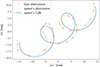 |
Fig. 1. Astrometric track of a binary system seen by Gaia. The solid blue line tracks the motion of the CoM of the system, while the dotted orange line tracks its photocentre. Individual Gaia scans of the sources are marked with solid orange lines aligned with the observation scanning angle. The goodness-of-fit of the CoM to the Gaia observations for this simulated system results in a RUWE of 2.07. |
2.1. RUWEs for binary systems
Estimating the RUWE for unresolved binary systems involves computing the separation between the photocentre and the CoM in the along-scan direction (AL), which will depend on both the Gaia observations and the configuration of the binary system, while considering the astrometric error (σast), which depends on the Gaia telescope configuration. As described in Lindegren (2022, see also Sect. 4.1 in Penoyre et al. 2022a), the equations governing a five-parameter solution for noisy observations are described by
 (1)
(1)
where ψ represents the scanning angle, τ = t − tref where t is the observation time in years and tref = 2016.0, PAL stands for the parallax factor, δη is the AL bias (derived from the projected AL separation between the CoM and the photocentre) and σast is the AL astrometric error. This system comprises nobs equations, where nobs is the number of CCD observations (source transits on Gaia’s focal plane typically generate nine CCD observations Gaia Collaboration 2016), and is solved for Δα*, Δδ, Δϖ, Δμα*, and Δμδ, which denote the expected biases arising from binarity (and will be zero for single-sources). From the residuals of these solutions, which quantify how much of the binary motion differs from the fitted single-source astrometric solution, we can compute the χ2 statistic, related to RUWE as
 (2)
(2)
We note that the RUWE reported in Gaia DR3 is a rescaled version of the original χ2 from AGIS (see Lindegren 2018, for further details).
The details from the Gaia scanning law necessary to estimate the RUWE of a particular system, determined by solving Eq. (1), are accessible through the Gaia Observation Schedule Tool (GOST3; Fernández-Hernández et al. 2022). GOST provides observation times, parallax factors, and scanning angles linked to a given set of sky coordinates. In our case, these coordinates correspond to the pixel centres at the HEALPix level 5 resolution observed between July 25, 2014, and May 28, 2017, covering the 34-month duration of Gaia DR3 observations. We chose the resolution at HEALPix level 5 to limit the computational cost of the calculations; however, the procedure described here and the examples shown in Appendix A are general for any spatial resolution. On the other hand, concerning the observed system, we needed to compute the projected AL separation between the system’s CoM and its photocentre at each observation time. This value is either zero (applicable for single sources, as discussed in Sect. 2.2) or computed based on the binary system configuration (as detailed in Sect. 3). Lastly, the AL astrometric error σast is determined as a function of the G magnitude, following the relationship provided in Lindegren et al. (2021b, see their Fig. A.1). To obtain its specific numerical value, we used the function sigma_ast available within the astromet python package4.
2.2. RUWE threshold for single stars
Section 2.1 describes the recipe to forward model the RUWE for a binary system based on its properties and location on-sky. However, to flag these binary systems we need to understand what RUWEs would describe a well-behaved single-source solution. For this, we characterised the maximum allowed RUWE, or the RUWE threshold, which will be compatible with single sources as a function of the sky coordinates. Following our approach, we estimated the RUWEs for a population of 105 simulated single sources located at the centres of each HEALPix at level 5 and observed under Gaia DR3. In this case, where the source’s CoM and photocentre follow identical tracks (δη = 0), the expected RUWE will be a χ distribution scaled by  , which for large n will approach a Gaussian with a dispersion that is proportional to the AL astrometric error. We assigned a magnitude to each simulated single source based on a uniform distribution within G ∈ (5, 20.7) mag, to cover the entire magnitude range. The corresponding σast value is computed based on this magnitude. Similar to the approach by Penoyre et al. (2022a, see their Fig. 4), we fitted a Student’s t-distribution to the resulting distribution of RUWE. From this distribution, we defined the maximum RUWE value compatible with the star being a single source, allowing for a one-in-a-million confusion rate, that is to say, solving for the RUWE where 1 − P(RUWE < τRUWE) = 10−6, where τRUWE is the computed RUWE threshold. This process was repeated 30 times to account for the random errors and to estimate an associated uncertainty (≤2 × 10⁻³) for this RUWE value. The final simulation-based RUWE threshold is the mean value of these 30 realisations.
2.2.1. Calibration with Gaia data
Up to this point we had focused on the methodology to calculate the RUWE for a Gaia observation of an isolated source, considering the presence or absence of an unseen companion. This methodology is particularly useful for modelling the RUWEs for unresolved binary systems and deriving general conclusions for this population (see Sect. 3). However, other sources’ properties such as stellar crowding, variability or the presence of disc material around single stars (among others, Belokurov et al. 2020; Fitton et al. 2022), or attitude and geometric calibration errors and other instrumental properties, also contribute to the increase in the sources’ RUWE (Lindegren 2018). In regions with particularly high stellar density, the observed single source might be influenced by neighbouring stars causing Gaia’s measured image to deviate from the single source point spread function model. This deviation leads to difficulties in accurately determining the point spread function’s centroid, resulting in an elevated RUWE.
A detailed modelling of the previous effects on the source’s RUWE is beyond the scope of this paper. Instead, we gauged these effects, specifically focusing on crowding, directly from the Gaia data employing the following approach. For HEALPix at level 5, we used scipy’s curve_fit function in Python5 to fit a Gaussian to the left half of the RUWE distribution of all the sources in the HEALPix retrieved from Gaia archive (left half with respect to the mode of the distribution, usually centred at one but automatically estimated from the data). Using the full Gaussian, representing a single-source population, we obtained the maximum RUWE allowed for single sources by applying the procedure described in Sect. 2.2. Figure 2 shows the RUWE distribution for the ∼106 sources in Gaia corresponding to the HEALPix centred at l = 73.58° and b = 3.17°. Additionally, we show the Gaussian distribution fitted to the sources centred around RUWE ∼1. In this case, the RUWE threshold for single sources estimated from both the simulated single-source population (see Sect. 2.2) and actual data are 1.14 and 1.22, respectively.
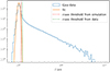 |
Fig. 2. Histogram of RUWEs for sources in the Gaia archive (blue line) HEALPix centred at l = 73.58°, b = 3.17°. The solid orange line indicates our fit of the single-source population in that HEALPix. The dotted lines indicate the RUWE thresholds for single sources with (green) and without (red) crowding effects. |
The data-driven approach adopted here faces limitations in its application across the whole sky due to the necessity of a minimum source count, and the RUWE distribution around its mode to be well represented by a Gaussian for an accurate fit. For HEALPix regions where we obtain a data-driven RUWE threshold, we fitted a second-order polynomial to the difference of the RUWE thresholds (i.e., τRUWEdata − τRUWEsimulation) as a function of the logarithm of the source count within that HEALPix. With this, we derived an adjustment factor, or offset, to refine the simulation-based RUWE threshold, accounting primarily for the influence of crowding based on the number of sources present within each HEALPix.
Figure 3 shows the estimated highest RUWE compatible with single-star solutions across the sky. It shows a strong dependence on the Gaia scanning law, indicating that regions with a higher number of observations tend to exhibit lower RUWE thresholds since the fitted AGIS solution for each source is better constrained. We also see the impact of crowding within the Galactic plane, especially towards the Galactic centre and the Magellanic Clouds. These regions show elevated RUWE thresholds due to challenges in reliably fitting the single source track using AGIS caused by the misidentification of sources due to their high stellar density. This misidentification for a large fraction of sources in those regions will cause the single-source RUWE distribution to be skewed towards RUWEs larger than one, resulting in a higher threshold value after our calibration.
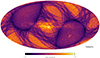 |
Fig. 3. Sky map of the sky-varying RUWE threshold at the resolution of HEALPix level 5. Sources above these RUWE thresholds are potential binary systems. These RUWEs show a strong influence from the Gaia scanning law, while also highlighting regions with high source density. |
The RUWE threshold variation across different sky coordinates presented in our work represents an improvement over prior studies that employed a singular RUWE value across the whole sky. For instance, in Gaia DR2, Lindegren (2018) suggested a RUWE threshold of 1.4 to characterise good Gaia solutions, with higher values potentially indicating binarity or other influencing factors. For Gaia EDR3, Penoyre et al. (2022a) investigated the imprints left in the RUWE distribution attributed to nearby binary systems (within 100 pc) and recommended a threshold of 1.25 for identifying potential binarity (the authors’ discussion focuses around LUWE, which stands for local renormalised UWE). The different RUWE thresholds suggested in different studies highlight the sensitivity of RUWE to different observational factors, their relation to specific Gaia data releases, for example DR2 or DR3, and the characteristics of the observed regions.
2.2.2. Selection probability of sources with high RUWEs
We computed the selection probability for sources in Gaia DR3 with RUWEs higher than the estimated RUWE threshold, using the approach described in Castro-Ginard et al. (2023) to estimate selection functions for Gaia subsamples. We note here that for a universe consisting only of single stars without any photocentre motion, and for perfectly behaved and calibrated Gaia instruments, by construction the probability of selecting sources above the RUWE threshold would be 10−6, independent of sky position or source brightness. In reality (as shown below) the selection probability is much higher and this can indicate, among others, the presence of unseen companions to the selected sources.
Within each HEALPix at level 5, we determined the expected selection probability as
 (3)
(3)
where k represents the count of sources exceeding the estimated sky-varying RUWE threshold (shown Fig. 3), and n is the total number of sources within that HEALPix. Figure 4 shows the estimated selection probability across the sky, revealing that the selection of these sources, which in some regions may translate to the detectability of binary systems defined as sources with large RUWEs, correlates with the Gaia scanning law. We see a higher selection probability in crowded areas, for example the Galactic plane, particularly towards the Galactic centre, and the Magellanic Clouds or the hot pixels correspond to the cores of globular clusters. We cannot interpret these high-selection probability regions as being highly populated by binary systems. As previously discussed, several reasons in both the sources or instrument properties can contribute to an increased RUWE. Therefore, these high-selection probability regions can be seen as regions with an important contribution from factors other than binarity that increase the sources’ RUWE, tracing regions of high contamination when binary systems are selected solely based on RUWE. In this paper, our modelling primarily focuses on the increase in RUWE caused by a bad single-source fit by AGIS due to the presence of an unresolved companion, which is typically the predominant contribution across most of the sky (i.e., Galactic latitudes above the plane and avoiding crowded regions). Consequently, selecting binary systems based on RUWE within highly crowded areas will include a higher level of contamination or interference from other contributing factors, even with our sky-varying RUWE threshold taking crowding into account.
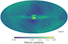 |
Fig. 4. Selection probability for sources with a RUWE higher than the threshold represented in Fig. 3. The regions with a higher selection probability, e.g., cores of globular clusters, the Galactic plane, and the Magellanic Clouds, contain sources with an increased RUWE due to a combination of binarity, source crowding, and other effects. These regions may indicate a higher contamination rate if binaries are selected solely based on RUWE. The dark halos around the Magellanic Clouds are due to an excess of faint sources with low RUWE in that region. |
3. Properties of detected binary systems
The approach presented in Sect. 2 allows us to estimate RUWEs for any source observed by Gaia, including unresolved binary systems, based on their properties and location on-sky. With this approach, and considering a specific population of binary systems, we can characterise what properties will enhance the probability of detection for unresolved binary systems in Gaia DR3, when detected as systems whose estimated RUWEs are higher than the threshold shown in Fig. 3.
3.1. Simulated binary population
We simulated a population of binary systems to predict their detectability as a function of the system’s parameters. This simulated population was not intended to mirror a realistic representation of binary systems distributed throughout the Galaxy. Instead, the simulation aimed to cover a broad range of stellar binary characteristics, for example mass and light ratios or orbital properties, that are general enough to allow for an exploration of the effect of the binary parameters on the probability of being selected based on the RUWE threshold, which varies across the sky.
We generated around 1 million MS binaries to study the detectability variations of different simulated parameters. First, we retrieved the stellar parameters from the PARSEC6 isochrones (Bressan et al. 2012) for a uniform grid of different ages. We isolated the isochrones’ MS and took the corresponding masses as the mass of the binary primary component. We assigned a mass ratio (q) following a uniform distribution from 0 to 1 to each of the primary masses to build a binary system. These systems were uniformly placed at varying distances ranging from 10 pc to 5 kpc. We calculated the Gaia’s G magnitude from the mass and distance distributions, assuming no extinction, and restricted our analysis to systems within Gaia’s observational limits (i.e. G < 20.7 mag). The remaining parameters for the simulated binaries followed the distributions described in Table 1 and are similar to those used in Penoyre et al. (2022a, their Table 1). The semi-major axis of the binary orbit was computed using the masses of both components and the orbital period. Finally, since we considered MS-MS binaries, the luminosity ratio was computed from the mass ratio as l = q3.5.
Distributions for the simulated binary system population.
3.2. Selection probability and binary system properties
We distributed the generated population of binary systems across various sky locations to evaluate the fraction of these systems that would be detected using RUWE (estimated as in Sect. 2.1). Figure 5 shows this detection fraction for the different binary configurations considered at the pixel centred at l = 15.3° and b = −14.4°, with yellow pixels representing a nearly complete detection while bluer pixels indicating a detection fraction closer to zero within that specific configuration. As expected, the binary detectability peaks at a mass ratio of q = 0.5. No systems are detected when q = 0 (equivalent to single sources), or when q = 1 where the CoM and the photocentre trace the same trajectory, which means the RUWE is not changed.
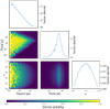 |
Fig. 5. Heatmap of binary systems’ properties, i.e. distances, periods, and mass ratios, that will increase their detectability. The detectability of these systems monotonically decreases with distance, reaching a detection fraction of 50% at around 100 pc. There is a strong detectability window around periods of three years, corresponding to the Gaia observation time baseline. Systems with mass ratios of 0, i.e., single sources, or 1 show no sign of binarity in the RUWE since there is no wobbling of their CoM around the photocentre. |
The detection probability shows a peak at an orbital period aligning with the observational baseline of the survey, which is 34 months for Gaia DR3. This probability gradually declines for longer periods, given that no observable orbital motion is evident within this observation time (Penoyre et al. 2020). Furthermore, we observe notable declines in the fraction of detected systems when the orbital period coincides harmonically with a year, prominently visible in Fig. 5 at periods of 1 year and 1/2 year. This decrease in detectability arises due to a confusion of the orbital motion with a parallax shift, leading to a situation where a seemingly good astrometric fit (resulting in a low RUWE) corresponds to an erroneous parallax. These features in the period distribution are also visible in the astrometric binaries in Gaia DR3 (Halbwachs et al. 2023, also selected based on the RUWE). We observed that the strength of this effect, however, depends on the direction of the observed binary systems (details of the Gaia scanning law).
From the first column in Fig. 5, we see that our ability to detect binary systems is monotonically decreasing with distance, reaching 50% of systems detected at around 100 pc. To capture the variation of this behaviour across different regions of the sky, we estimated the RUWE of the simulated binary population described in Sect. 3.1 in different pixels from the north to the south ecliptic poles at ecliptic longitude λ = 0°, and from λ = 0° to λ = 360° at ecliptic latitude β = 0°, as shown in Fig. 6. We used ecliptic coordinates since the Gaia scanning law is symmetric in this coordinate system and is the strongest contribution to the variation in the RUWE threshold across the sky (see Sect. 2.2). Also, we focused on periods from one to four years, which is the window for optimal detectability, since most of the selected binary systems will be in this period range (see the discussion in Sect. 4). Figure 6 shows how the variation of the distance where 50% of the simulated systems are detected (where the median RUWE is equal to the RUWE threshold shown in Fig. 3). We see that in the ecliptic poles, and up to |β| = 45°, where Gaia has uniformly scanned the sky with a large number of observations, we can detect binary systems at larger distances (up to around 1 kpc) due to a more constrained astrometric solution, thus resulting in a lower RUWE. For the |β|< 45°, on the other hand, the distance where we detect at least 50% of the simulated binary systems can decrease down to 800 pc. Along the λ direction, the distance reached shows a more irregular behaviour since this region captures larger variations in the Gaia scanning law. However, the distances where we can detect systems can vary ∼200 pc depending on the scanning configurations. If we include in the analysis the whole range of simulated periods, the distances where we detect 50% of the simulated systems range from around 60 up to 150 pc, approximately, depending on the (λ, β) direction.
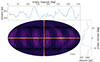 |
Fig. 6. Central panel: same as Fig. 3 but in ecliptic coordinates. The pixels highlighted in the vertical and horizontal directions show the regions where we estimate the maximum distance at which we detect half of the simulated systems, as shown in the right and top panels, respectively. Top panel: distance at which 50% of the systems are detected, for the highlighted pixels along the ecliptic λ = 0°. Right panel: same as the top panel but for ecliptic β = 0°. |
4. The GCNS binary population through GUMS
Gaia Collaboration (2021b) produced a catalogue of 331 312 objects within 100 pc that was released together with Gaia EDR3. The catalogue includes a list of probable members of the two closest open clusters (i.e., the Hyades and Coma Berenices), white dwarfs (WDs), and resolved binary systems. It also includes numerous sources with RUWEs significantly higher than 1, which may be potential unresolved binary systems that may have gone unnoticed. We find 74 785 potential unresolved binary systems with a catalogued RUWE higher than the threshold for single sources we computed in Sect. 2.2 (see Fig. 3). Based on our approach, we can select more binary system candidates compared to the selection based on RUWEs higher than 1.4 and 1.25, which provide 55 754 and 70 848, respectively. In Fig. 7 we show how our selection of unresolved binary systems is distributed in a colour–magnitude diagram (probability estimated as in Eq. (3) with respect to the colour and magnitude bins). We observe a high selection probability in the brighter MS, which monotonically decreases towards faint magnitudes. A similar trend is observed in the WD sequence (10 ≲ MG ≲ 15 and 0 ≲ GBP − GRP ≲ 1), where the selection probability is higher in the brighter sequence. The region between the MS and the WD sequence, which shows a selection probability unexpectedly high, corresponds to sources with ‘poor astrometric solutions’ in the GCNS catalogue (see Sect. 2.1 in Gaia Collaboration 2021b, for further details). Although this region also contains MS-WD binaries, the RUWE for the sources in this region is probably also increased for reasons other than binarity. Therefore, this region may represent a highly contaminated region in our analysis.
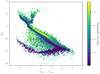 |
Fig. 7. Selection probability of the GCNS sources with RUWEs larger than our threshold shown in Fig. 3 across the colour–magnitude diagram. For the MS and WD sequence, we see a gradient on the selection probability for bins at the same GBP − GRP colour. The region between the MS and the WD sequence, which contains the MS–WD binaries, has a high concentration of sources marked as having poor astrometric solutions in the GCNS. |
To understand the completeness and contamination of this sample, and the types of systems that our method selects among the unresolved binary system candidates, we used the Gaia Universe Model Snapshot (GUMS; Robin et al. 2012). GUMS provides astrometry, through the Gaia Object Generator (GOG; Luri et al. 2014), photometry and astrophysical parameters of sources as if they were observed by Gaia. GUMS only provides around 100 000 sources within 100 pc. Therefore, to increase the statistical significance of the analysis, we increased the volume to analyse to 200 pc, resulting in 882 107 sources, of which 243 377 are true binary systems.
We forward-modelled the RUWE for these GUMS sources following the recipe in Sect. 2.1 (see Appendix A for instructions on how to use our GaiaUnlimited Python package). Then, we detected these binary systems based on RUWE as we did for the GCNS. We recover 51 524 true binary systems with our variable RUWE approach, which still results in a more complete sample when compared to selections on RUWE higher than 1.4 and 1.25, resulting in 43 398 and 50 431, respectively. The contamination of our sample is one single source selected as a binary system, as expected by the design of our approach (see Sect. 2.2). This contamination is zero in the case of a RUWE > 1.4, due to the more restrictive criteria, and 20 in the case of a RUWE > 1.25. Therefore, our approach provides a sample of unresolved binary systems with the best compromise between completeness and contamination when compared to other criteria to select this type of object.
Working with simulated data has the advantage that we can access all the true simulated parameters. In this case, we can study the population of binary systems depending on the evolutionary stages of their two components. We identified five main evolutionary stages present in GUMS: giant stars, WDs, and high-, low-, and mid-MS stars, defined as stars with MG < 4, MG > 10, and in between these cuts, respectively. Figure 8 shows the distribution of mass and light ratios for GUMS binaries within 200 pc, as well as the subset that are unresolved and have a detectable excess RUWE. This shows the range of important (though often not observable) physical properties we might expect from a range of binary systems. MS stars, especially those that are cooler and of lower mass, follow a relatively tight distribution (akin to our previous heuristic of l ∝ q3.5), above this (and thus closer in light ratio for a given mass ratio) we see binaries containing stars the mass and temperature of our Sun and higher, which are significantly less tightly clustered but follow a similar trend. Systems that contain giants generally fall below these populations (as the giant primary is effectively over-luminous for its mass). Systems that contain WDs, having generally much more mass compared to their luminosity (except for WD–WD binaries which cluster very close to q ≈ 1 and l ≈ 1) are distinct in this space.
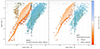 |
Fig. 8. Mass and light ratios of a random subset of 30 000 (of 242 485) binaries from GUMS within 200 pc. The central colour of each point shows the type of the primary, and the outline shows the type of the secondary. MS stars are given a colour that approximately corresponds to their visual colour based on their effective temperature. Giants (MG < 4 and GBP − GRP > 0.9) are shown in dark red and WDs (MG − 3(GBP − GRP) < 9.5) in blue. The left panel shows all random binaries and the right panel only those that are unresolved and whose RUWE is greater than the threshold for their region of the sky. Because we chose the primary to be the brighter component (l < 1 always), the populations are effectively reflected through l = 1 and |

The strong dependence of light ratio on mass ratio leads to many unresolved binary systems being indistinguishable from single objects from their luminosity (and also in general from their spectra) as even moderate mass ratios, for example q = 0.5, lead to much smaller light ratios (l < 0.1). Thus, the light ratio, though crucial for fully characterising binary systems, is rarely measurable.
Comparing the full population to the detectable we can get a feeling for which kinds of systems are easier or more difficult to pick out from astrometry alone. We can see a low detection fraction for systems with Δ close to zero (as the astrometric motion is negligible), which includes both ‘twin’ systems (q ∼ l ∼ 1) and faint MS–MS and MS-giant binaries (with q ≲ 0.1). The detection fraction is also low for systems containing WDs where the second component is similarly or less luminous (top left of each panel, because these are dim enough that the astrometric error is high enough to dominate over astrometric motion).
4.1. Detectability functions with period and distance
Figure 9 shows the fraction of binaries that are detected as a function of period, expanding on Fig. 15 of Penoyre et al. (2022a). This is a very strong ‘window function’ limiting us to only binaries for which we see a significant fraction of the orbit (P ≲ 10 years, with the fraction dropping as P−2) and those whose orbits are wide enough that the astrometric motion is significant compared to the astrometric error (P ≳ 1 month, with the fraction increasing proportional to  ; see Penoyre et al. 2020, 2022a; Andrew et al. 2022, for more detail).
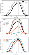 |
Fig. 9. Fraction of detectable binaries as a function of period, comparing the full population (within 200 pc) to subsets. Top panel: detectability within some distance range. Middle panel: detectability dependent on the type of the primary. Bottom panel: detectability dependent on the type of the secondary. The vertical line at 34 months shows the time baseline of Gaia DR3 (and is the optimal period for binary detection). MS stars are split into three subgroups: high (MG < 4), low (MG > 10) and mid (in between these two cuts). Around 15% of MS primaries fall into the high bin and another 15% into the low bin. Close to half of the secondaries are low, and the vast majority of the rest are mid (the number of high-mass MS secondaries is small, and giant secondaries are negligible). |
Even for a sample out to 200 pc (which will be dominated by the number of systems close to that distance limit), we detect more than 80% of systems at the optimal period of 34 months (Gaia DR3’s time baseline). For a closer limiting distance that fraction increases mostly due to the larger apparent magnitude and parallax, both leading to the astrometric signal being more dominant over astrometric noise.
Separating systems by the type of the primary we see essentially the same curve, with brighter primaries more easily detectable (again because of the reduced astrometric noise). Low mass primaries are significantly harder to detect (as the orbit is smaller for the same period) and so are WD primary systems (as these are necessarily low luminosity). The most massive primaries, especially the giants, are even more strongly peaked in period, particularly at the low period end. This is mostly a general astronomical bias rather than an astrometric one, since these are both rarer (thus they do not appear in significant numbers at small distances and smaller period orbits can be unresolvable at larger distances) and more limited in their minimum period by their large stellar radii and the requirement that the stars do not merge. Comparing instead the detectability based on the type of the secondary we now see that WD companions give significantly larger signals (because of their large q and low l, giving large Δ). In general, it is not a bad assumption that each of the curves shown here is a simple rescaling of the distribution across all stars, with the small caveat that it must saturate at a detection fraction of 1. Figure 10 shows a similar detectability function but now as a function of distance. All populations generally have lower detection fractions at increasing distances, where they are both smaller orbits on-sky and dimmer, and thus the astrometric error can increase.
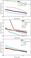 |
Fig. 10. Same as Fig. 9 but organised by the distance of the binary. We show the function for all systems in the sample and for subsamples separated by binary period (top), type of primary (middle), and type of secondary (bottom). |
Evidently, both the period and distance functions apply to the data at once, so we started by showing the detectable distance fraction split by period. For ideal periods (close to the peak at 34 months), the detectable fraction is close to 1 at small distances and still near 80% at the edge of our sample – as shown in Fig. 6 this will only drop below 50% for sources ∼1 kpc and farther. Longer-period systems are harder to detect but follow the same kind of behaviour, whilst short-period systems drop off non-linearly as the population approaches the astrometric noise floor of Gaia. Separating by primary type we see that dim primaries (WDs and low-MS stars) also drop off quickly with distance for the same reason, and more massive brighter systems follow the general trend. Finally, separating by secondary type, we again see that WD companions are the easiest to detect, but the slope of the detection fraction with distance does not depend on the secondary type.
For all of these systems, the limiting factor with distance is the ratio of the magnitude of the astrometric motion to the astrometric error, which will necessarily decrease with distance. For populations for which no sources remain in the (approximately) constant regime of astrometric error (G ≳ 13), this ratio drops more rapidly and thus the curve steepens. We would expect this steepening to apply to all types of sources eventually, modulated by their inherent luminosity, and thus the brightest giants may still be detectable as binaries at large distances (> 1 kpc). This estimation does not account for extinction and crowding increasing with distance, both of which will cause extra astrometric noise and may lower the distance at which binary detection is achievable, especially in crowded and obscured regions such as the Galactic disc, Galactic centre, and the Magellanic Clouds.
5. Summary and conclusions
In this study we have focused on the capability to detect unresolved binary systems in Gaia DR3, using the RUWE as the key metric. We developed a forward model for predicting the RUWEs, which depend on the sky coordinates and a set of astrophysical properties of the observed stellar system (single or binary). This model allowed us to determine the highest RUWE that will describe good Gaia measurements for single sources. Consequently, we established a RUWE threshold that varies across different regions of the sky (Fig. 3); RUWEs higher than this threshold indicate the potential presence of an unseen companion. Then, using the approach described in Castro-Ginard et al. (2023) to estimate the selection function of subsamples of Gaia data, we estimated the selection probability of a Gaia source with a RUWE above our sky-dependent threshold. We note that this selection probability will trace areas where binary systems can be more, or less, easily detected across most of the sky, except in very crowded regions. Figure 4 traces the contamination in these areas when selecting binary systems solely based on RUWE, since this will be increased due to contributions other than binarity.
We simulated a broad range of binary systems to describe what system characteristics, for example mass and luminosity ratios, periods, or distances, will lead to a RUWE above the threshold and therefore make these systems detectable using this approach. The probability of detecting these systems decreases with increasing distance. Specifically, about 50% of the simulated binary systems were detectable at a distance of approximately 100 pc. However, for binary systems with orbital periods as long as the temporal baseline of the survey, this detectability range extends significantly, allowing for the detection of half of these systems at distances of up to about 1 kpc. We also see that the impacts of binarity on the RUWE are weaker for systems with orbital periods around 1 or 1/2 years (due to a confusion with a parallax shift; Penoyre et al. 2020) and mass ratios going to 0 (single source) or 1 (no apparent wobbling of the photocentre around the CoM). Therefore, systems with these characteristics are less likely to be identified as binaries in Gaia when relying exclusively on the RUWE criteria.
Finally, we used the GUMS simulation within 200 pc and applied our forward model for the RUWE, to provide insight into the unresolved binary population in the GCNS. Our sky-varying RUWE criteria for identifying potential binary systems outperform the widely used threshold value of 1.4, both in terms of the completeness and the purity of the resulting sample. In the GUMS sample, we find that the most numerous binary systems, when both components are MS stars, are not the easiest to detect with Gaia. The strongest impact on the RUWE, which results in a higher detectability, is generated by binary systems with a luminous primary component (a high-MS, mid-MS, or giant star). On the other hand, binary systems with a dim primary component (a WD or low-MS star) will have a low detection probability. For instance, only about 1% of WD–WD binary systems simulated in GUMS were detected.
This study provides a new definition of what impacts on RUWE we can expect from binarity, and it is adapted to the systems’ location on-sky. However, most of the existing binary systems in our Galaxy will still go undetected due to the CoM wobbling around the photocentre being dominated by the astrometric noise of Gaia, therefore resulting in a RUWE value below the threshold. The tools we have developed are a valuable resource for detecting binary system candidates in Gaia data and characterising the properties of the population from which the selected systems are drawn. Following the example of previous GaiaUnlimited selection functions, we have made the code and tools generated in this work publicly available through the GaiaUnlimited Python package.
Acknowledgments
We thank David W. Hogg for his contributions to the GaiaUnlimited project. We thank Douglas Boubert, Andrew Everall and Tereza Jerabkova for their help in preparing the GUMS binary catalogue. This work is a result of the GaiaUnlimited project, which has received funding from the European Union’s Horizon 2020 research and innovation program under grant agreement No 101004110. The GaiaUnlimited project was started at the 2019 Santa Barbara Gaia Sprint, hosted by the Kavli Institute for Theoretical Physics at the University of California, Santa Barbara. ZP acknowledges that this project has received funding from the European Research Council (ERC) under the European Union’s Horizon 2020 research and innovation programme (Grant agreement No. 101002511 – VEGA P). This work has made use of results from the European Space Agency (ESA) space mission Gaia, the data from which were processed by the Gaia Data Processing and Analysis Consortium (DPAC). Funding for the DPAC has been provided by national institutions, in particular, the institutions participating in the Gaia Multilateral Agreement. The Gaia mission website is https://www.cosmos.esa.int/web/gaia. The authors are current or past members of the ESA Gaia mission team and of the Gaia DPAC. This work made use of Astropy (http://www.astropy.org): a community-developed core Python package and an ecosystem of tools and resources for astronomy (Astropy Collaboration 2022).
References
- Andrew, S., Penoyre, Z., Belokurov, V., Evans, N. W., & Oh, S. 2022, MNRAS, 516, 3661 [NASA ADS] [CrossRef] [Google Scholar]
- Astropy Collaboration (Price-Whelan, A. M., et al.) 2022, ApJ, 935, 167 [NASA ADS] [CrossRef] [Google Scholar]
- Belokurov, V., Penoyre, Z., Oh, S., et al. 2020, MNRAS, 496, 1922 [Google Scholar]
- Bressan, A., Marigo, P., Girardi, L., et al. 2012, MNRAS, 427, 127 [NASA ADS] [CrossRef] [Google Scholar]
- Cantat-Gaudin, T., Fouesneau, M., Rix, H.-W., et al. 2023, A&A, 669, A55 [NASA ADS] [CrossRef] [EDP Sciences] [Google Scholar]
- Cantat-Gaudin, T., Fouesneau, M., Rix, H. W., et al. 2024, A&A, 683, A128 [NASA ADS] [CrossRef] [EDP Sciences] [Google Scholar]
- Castro-Ginard, A., Brown, A. G. A., Kostrzewa-Rutkowska, Z., et al. 2023, A&A, 677, A37 [NASA ADS] [CrossRef] [EDP Sciences] [Google Scholar]
- Duchêne, G., & Kraus, A. 2013, ARA&A, 51, 269 [Google Scholar]
- Duchêne, G., Lacour, S., Moraux, E., Goodwin, S., & Bouvier, J. 2018, MNRAS, 478, 1825 [NASA ADS] [Google Scholar]
- El-Badry, K. 2024, New Astron., accepted [arXiv:2403.12146] [Google Scholar]
- El-Badry, K., Rix, H.-W., & Heintz, T. M. 2021, MNRAS, 506, 2269 [NASA ADS] [CrossRef] [Google Scholar]
- Fernández-Hernández, J., Joliet, E., & Garralda, N. 2022, GOST Software User Manual, https://gaia.esac.esa.int/gost/docs/gost_software_user_manual.pdf [Google Scholar]
- Fitton, S., Tofflemire, B. M., & Kraus, A. L. 2022, Res. Notes Am. Astron. Soc., 6, 18 [Google Scholar]
- Gaia Collaboration (Prusti, T., et al.) 2016, A&A, 595, A1 [NASA ADS] [CrossRef] [EDP Sciences] [Google Scholar]
- Gaia Collaboration (Brown, A. G. A., et al.) 2018, A&A, 616, A1 [NASA ADS] [CrossRef] [EDP Sciences] [Google Scholar]
- Gaia Collaboration (Brown, A. G. A., et al.) 2021a, A&A, 649, A1 [NASA ADS] [CrossRef] [EDP Sciences] [Google Scholar]
- Gaia Collaboration (Smart, R. L., et al.) 2021b, A&A, 649, A6 [EDP Sciences] [Google Scholar]
- Gaia Collaboration (Vallenari, A., et al.) 2023, A&A, 674, A1 [NASA ADS] [CrossRef] [EDP Sciences] [Google Scholar]
- Halbwachs, J.-L., Pourbaix, D., Arenou, F., et al. 2023, A&A, 674, A9 [NASA ADS] [CrossRef] [EDP Sciences] [Google Scholar]
- Kervella, P., Arenou, F., & Thévenin, F. 2022, A&A, 657, A7 [NASA ADS] [CrossRef] [EDP Sciences] [Google Scholar]
- Lindegren, L. 2018, GAIA-C3-TN-LU-LL-124 [Google Scholar]
- Lindegren, L. 2022, GAIA-C3-TN-LU-LL-136 [Google Scholar]
- Lindegren, L., Bastian, U., Biermann, M., et al. 2021a, A&A, 649, A4 [EDP Sciences] [Google Scholar]
- Lindegren, L., Klioner, S. A., Hernández, J., et al. 2021b, A&A, 649, A2 [EDP Sciences] [Google Scholar]
- Luri, X., Palmer, M., Arenou, F., et al. 2014, A&A, 566, A119 [NASA ADS] [CrossRef] [EDP Sciences] [Google Scholar]
- Majewski, S. R., Schiavon, R. P., Frinchaboy, P. M., et al. 2017, AJ, 154, 94 [NASA ADS] [CrossRef] [Google Scholar]
- Penoyre, Z., Belokurov, V., Wyn Evans, N., Everall, A., & Koposov, S. E. 2020, MNRAS, 495, 321 [NASA ADS] [CrossRef] [Google Scholar]
- Penoyre, Z., Belokurov, V., & Evans, N. W. 2022a, MNRAS, 513, 2437 [NASA ADS] [CrossRef] [Google Scholar]
- Penoyre, Z., Belokurov, V., & Evans, N. W. 2022b, MNRAS, 513, 5270 [Google Scholar]
- Price-Whelan, A. M., Hogg, D. W., Rix, H.-W., et al. 2020, ApJ, 895, 2 [NASA ADS] [CrossRef] [Google Scholar]
- Raghavan, D., McAlister, H. A., Henry, T. J., et al. 2010, ApJS, 190, 1 [Google Scholar]
- Robin, A. C., Luri, X., Reylé, C., et al. 2012, A&A, 543, A100 [NASA ADS] [CrossRef] [EDP Sciences] [Google Scholar]
- Skrutskie, M. F., Cutri, R. M., Stiening, R., et al. 2006, AJ, 131, 1163 [NASA ADS] [CrossRef] [Google Scholar]
- Stassun, K. G., & Torres, G. 2021, ApJ, 907, L33 [NASA ADS] [CrossRef] [Google Scholar]
- Wallace, A. L. 2024, MNRAS, 527, 8718 [Google Scholar]
- Wright, E. L., Eisenhardt, P. R. M., Mainzer, A. K., et al. 2010, AJ, 140, 1868 [Google Scholar]
Appendix A: Using the GaiaUnlimited python package
We provide the code we used to estimate the selection function of binary systems as a new tool in the GaiaUnlimited python package7. The data needed to generate the plots in the paper (i.e. all-sky scanning law details at a HEALPix level 5 resolution) are also included within the package.
Listing 1 shows how to use the new BinarySystemsSelectionFunction class. Similarly to the previous GaiaUnlimited selection functions, it takes an astropy coordinate object and returns the queried quantity, for example the sky-varying RUWE threshold (to produce Fig 3) and selection probabilities of sources with high RUWEs (computed as in Castro-Ginard et al. 2023, produces Fig. 4) or Gaia scanning law details.
1  from gaiaunlimited.selectionfunctions import binaries
2
3  SF = binaries.BinarySystemsSelectionFunction()
4
5  from astropy import units as u
6  from astropy.coordinates import SkyCoord
7
8  coord = SkyCoord(ra = ra*u.degree , dec = dec*u.degree , frame = 'icrs')
9
10 # Generates the selection probabilities based on RUWE.
11 # Function to generate Fig. 4.
12 probability ,variance = SF.query(coord , return_variance = True)
13
14 # Returns the RUWE threshold above which a source is considered a potential binary system.
15 # Function to generate Fig. 3.
16 the RUWE = SF.query_the RUWE(coord ,crowding = True)
Listing 1. Example of code to initialise and query the selection function of binary systems.
We also provide our forward model for computing the RUWE from the binary system properties, and the Gaia scanning law in the SimulateGaiaSource class. Listing 2 shows how to initialise the simulation of a system at a given sky location, providing the period, eccentricity and initial phase of the system, as well as the Gaia scanning law details (observation times, scanning angles and parallax factors, provided by GOST). The AL measurements and errors are computed as a function of the other system properties. Finally, the RUWE was computed from these simulated observations. Full documentation of the package is available through the GaiaUnlimited documentation website8.
1  from gaiaunlimited.utils import SimulateGaiaSource
2
3  source = SimulateGaiaSource(ra, dec, period , eccentricity , initial_phase)
4
5  al_pos ,al_err = source.observe(Gmag ,
6    parallax ,
7    semimajor_axis ,
8    mass_ratio ,
9    luminosity_ratio ,
10    phi,
11    theta ,
12    omega ,)
13
14 ruwe= source.unit_weight_error(al_pos , al_err)
Listing 2. Example of code to simulate a Gaia observation as a function of the source parameters (single or binary) and estimate its RUWE.
All Tables
All Figures
|
Fig. 1. Astrometric track of a binary system seen by Gaia. The solid blue line tracks the motion of the CoM of the system, while the dotted orange line tracks its photocentre. Individual Gaia scans of the sources are marked with solid orange lines aligned with the observation scanning angle. The goodness-of-fit of the CoM to the Gaia observations for this simulated system results in a RUWE of 2.07. |
| In the text | |
|
Fig. 2. Histogram of RUWEs for sources in the Gaia archive (blue line) HEALPix centred at l = 73.58°, b = 3.17°. The solid orange line indicates our fit of the single-source population in that HEALPix. The dotted lines indicate the RUWE thresholds for single sources with (green) and without (red) crowding effects. |
| In the text | |
|
Fig. 3. Sky map of the sky-varying RUWE threshold at the resolution of HEALPix level 5. Sources above these RUWE thresholds are potential binary systems. These RUWEs show a strong influence from the Gaia scanning law, while also highlighting regions with high source density. |
| In the text | |
|
Fig. 4. Selection probability for sources with a RUWE higher than the threshold represented in Fig. 3. The regions with a higher selection probability, e.g., cores of globular clusters, the Galactic plane, and the Magellanic Clouds, contain sources with an increased RUWE due to a combination of binarity, source crowding, and other effects. These regions may indicate a higher contamination rate if binaries are selected solely based on RUWE. The dark halos around the Magellanic Clouds are due to an excess of faint sources with low RUWE in that region. |
| In the text | |
|
Fig. 5. Heatmap of binary systems’ properties, i.e. distances, periods, and mass ratios, that will increase their detectability. The detectability of these systems monotonically decreases with distance, reaching a detection fraction of 50% at around 100 pc. There is a strong detectability window around periods of three years, corresponding to the Gaia observation time baseline. Systems with mass ratios of 0, i.e., single sources, or 1 show no sign of binarity in the RUWE since there is no wobbling of their CoM around the photocentre. |
| In the text | |
|
Fig. 6. Central panel: same as Fig. 3 but in ecliptic coordinates. The pixels highlighted in the vertical and horizontal directions show the regions where we estimate the maximum distance at which we detect half of the simulated systems, as shown in the right and top panels, respectively. Top panel: distance at which 50% of the systems are detected, for the highlighted pixels along the ecliptic λ = 0°. Right panel: same as the top panel but for ecliptic β = 0°. |
| In the text | |
|
Fig. 7. Selection probability of the GCNS sources with RUWEs larger than our threshold shown in Fig. 3 across the colour–magnitude diagram. For the MS and WD sequence, we see a gradient on the selection probability for bins at the same GBP − GRP colour. The region between the MS and the WD sequence, which contains the MS–WD binaries, has a high concentration of sources marked as having poor astrometric solutions in the GCNS. |
| In the text | |
|
Fig. 8. Mass and light ratios of a random subset of 30 000 (of 242 485) binaries from GUMS within 200 pc. The central colour of each point shows the type of the primary, and the outline shows the type of the secondary. MS stars are given a colour that approximately corresponds to their visual colour based on their effective temperature. Giants (MG < 4 and GBP − GRP > 0.9) are shown in dark red and WDs (MG − 3(GBP − GRP) < 9.5) in blue. The left panel shows all random binaries and the right panel only those that are unresolved and whose RUWE is greater than the threshold for their region of the sky. Because we chose the primary to be the brighter component (l < 1 always), the populations are effectively reflected through l = 1 and |
| In the text | |
|
Fig. 9. Fraction of detectable binaries as a function of period, comparing the full population (within 200 pc) to subsets. Top panel: detectability within some distance range. Middle panel: detectability dependent on the type of the primary. Bottom panel: detectability dependent on the type of the secondary. The vertical line at 34 months shows the time baseline of Gaia DR3 (and is the optimal period for binary detection). MS stars are split into three subgroups: high (MG < 4), low (MG > 10) and mid (in between these two cuts). Around 15% of MS primaries fall into the high bin and another 15% into the low bin. Close to half of the secondaries are low, and the vast majority of the rest are mid (the number of high-mass MS secondaries is small, and giant secondaries are negligible). |
| In the text | |
|
Fig. 10. Same as Fig. 9 but organised by the distance of the binary. We show the function for all systems in the sample and for subsamples separated by binary period (top), type of primary (middle), and type of secondary (bottom). |
| In the text | |
Current usage metrics show cumulative count of Article Views (full-text article views including HTML views, PDF and ePub downloads, according to the available data) and Abstracts Views on Vision4Press platform.
Data correspond to usage on the plateform after 2015. The current usage metrics is available 48-96 hours after online publication and is updated daily on week days.
Initial download of the metrics may take a while.