| Issue |
A&A
Volume 688, August 2024
|
|
|---|---|---|
| Article Number | A143 | |
| Number of page(s) | 19 | |
| Section | Stellar structure and evolution | |
| DOI | https://doi.org/10.1051/0004-6361/202349014 | |
| Published online | 12 August 2024 | |
SiO maser polarization and magnetic field in evolved cool stars
1
Laboratoire d’astrophysique de Bordeaux, Univ. Bordeaux, CNRS, B18N, allée Geoffroy Saint-Hilaire, 33615 Pessac, France
e-mail: This email address is being protected from spambots. You need JavaScript enabled to view it.
2
Max-Planck-Institut für Radioastronomie, Auf dem Hügel 69, 53121 Bonn, Germany
3
IRAP, Université de Toulouse, CNRS, CNES, UPS, 14 Av. E. Belin, 31400 Toulouse, France
4
Instituto de Astrofísica de Canarias, La Laguna, Spain
5
LUPM, Université de Montpellier, CNRS, place Eugène Bataillon, 34095 Montpellier, France
6
IRAP, Université de Toulouse, CNRS, UPS, CNES, 57 avenue d’Azereix, 65000 Tarbes, France
7
LESIA, Observatoire de Paris, Université PSL, CNRS, Sorbonne Université, Université Paris Cité, 5 place Jules Janssen, 92195 Meudon, France
Received:
19
December
2023
Accepted:
16
May
2024
Abstract
Context. Magnetic fields, photospheric and atmospheric dynamics can be involved in triggering the high mass loss observed in evolved cool stars. Previous works have revealed that the magnetic field of these objects extends beyond their surface. The origin of this magnetic field is still debated. The possible mechanisms include a turbulent dynamo, convection, stellar pulsation, and cool spots.
Aims. Our goal is to estimate the magnetic field strength in the inner circumstellar envelope of six evolved cool stars (five Miras and one red supergiant). Combining this work with previous studies, we tentatively constrain the global magnetic field type and shed light on the mechanisms that cause it.
Methods. Using the XPOL polarimeter installed at the IRAM-30 m telescope, we observed the 28SiO v = 1, J = 2 − 1 maser line emission and obtained simultaneous spectroscopic measurements of the four Stokes parameters. Applying a careful calibration method for Stokes Q, U, and V, we derived estimates of the magnetic field strength from the circular and linear polarization fractions considering the saturated and unsaturated maser cases under the Zeeman hypothesis.
Results. Magnetic field strengths from several Gauss up to several dozen Gauss are derived. These new and more accurate measurements constrain the field strength in the region of 2–5 stellar radii better than previous studies and appear to exclude a global poloidal magnetic field type. The combination of a toroidal and poloidal field is not excluded, however. A variation in the magnetic field strength over a two-month timescale is observed in one Mira star, which suggests a possible link to the stellar phase, that is, a link with pulsation and photospheric activity.
Key words: magnetic fields / masers / polarization / stars: evolution / stars: late-type / stars: magnetic field
© The Authors 2024
 Open Access article, published by EDP Sciences, under the terms of the Creative Commons Attribution License (https://creativecommons.org/licenses/by/4.0), which permits unrestricted use, distribution, and reproduction in any medium, provided the original work is properly cited.
This article is published in open access under the Subscribe to Open model. This email address is being protected from spambots. You need JavaScript enabled to view it. to support open access publication.
1. Introduction
After leaving the main sequence, solar-type stars (0.8–8 M⊙ ) go through different phases prior to the planetary nebula stage (e.g. Herwig 2005). The asymptotic giant branch (AGB) phase lasts less than a few million years, but is one of the most interesting phases in terms of chemistry and dynamics. Beyond the photosphere, AGB objects harbor a true chemical factory in their circumstellar envelope (hereafter CSE), where more than 80 molecules and 15 dust species have been discovered (Höfner & Olofsson 2018; Decin et al. 2018). This AGB phase is also characterized by a massive mass loss (10−6 − 10−4 M⊙ yr−1, Höfner & Olofsson 2018) that makes these objects the main contributors to the chemical enrichment of the interstellar medium and to the recycling of matter in the Universe. This also applies to their massive counterparts, the red supergiants (RSG, Ekström et al. 2012; De Beck et al. 2010).
Evolved cool stars therefore provide strong mechanical and radiative feedback to their host environment (Langer 2012). The high mass-loss rates of AGB stars are thought to be the result of a wind acceleration mechanism that is based on radiation pressure on dust grains that formed in the inner part of the CSE (at a few stellar radii) and are lifted by stellar pulsation (Bladh & Höfner 2012). No consistent scenario exists for RSGs. The exact mechanisms that trigger and shape the strong winds of evolved cool stars still need further characterization. This requires deeper studies of the subphotospheric layers where convection and pulsation act, of the atmosphere where strong radiating shocks occur, and of the wind-forming region where dust condensates and radiation acceleration occuts. In addition to the stellar convection, pulsation, and radiation pressure on dust, it has been proposed that magnetic fields play a significant role through Alfvén-wave driving of the wind (see for instance, Cranmer & Saar 2011; Höfner & Olofsson 2018), but that they also shape the wind (see Pascoli & Lahoche 2008; Dorch 2004, for pulsating evolved stars (AGBs) and for RSGs, respectively). If the fields are strong enough, they could even help to extract the angular momentum (cf. the case of the cool main sequence stars, Bouvier 2009). Magnetism and photospheric dynamics therefore both contribute in sustaining winds (Lèbre et al. 2014, 2015; López Ariste et al. 2019), but the relative importance of the magnetic field for the photospheric and atmospheric dynamics is still poorly known. The knowledge of the magnetic field strength and geometry is still limited. The origin of the magnetic field strength as a possible astrophysical dynamo in these stars would most likely be very different from the dynamo (α − ω) that is at work in solar-type stars because these rotate slowly, and only a few convection cells are present at their surface at any given time (Freytag et al. 2002; Aurière et al. 2010). For these slow rotators (with high Rossby number, up to ∼100, Charbonnel et al. 2017; Josselin et al. 2015), classical α − ω dynamos in which the toroidal component of the magnetic field is amplified by rotation are indeed not expected. On the contrary, a turbulent (convective) dynamo (α2 − ω) can generate a local weak magnetic field up to 0.01 Gauss, which is then amplified by stellar pulsation and cool spots to a large-scale magnetic field (Soker 2002). In the case of RSGs, a local small-scale dynamo generating a strong field with a small filling factor is favored based on numerical simulations (Dorch 2004). While convection cannot generate global magnetic fields, local fields therefore remain possible and may lead to the generation of (at least) local episodic mass-loss events (such as the one observed on Betelgeuse by Montargès et al. 2021).
Low-intensity magnetic fields (of about 1–10 Gauss at the stellar surface or at a few stellar radii) have been identified and monitored over several years in RSGs and AGBs. In the past decade, modern optical spectropolarimeters ESPaDOnS/CFHT1 and Narval/TBL) have brought much information about the stellar surface magnetism in the Hertzsprung–Russel diagram (e.g., Aurière et al. 2010; Lèbre et al. 2014; Tessore et al. 2017). In the radio regime, the polarimetric estimation of the magnetic field strength in the CSE of evolved stars has been possible, for instance, through the XPOL instrument at the IRAM-30m (e.g., Herpin et al. 2006), the VLBA array (e.g., Kemball et al. 2011; Assaf et al. 2013), or now with ALMA (e.g., Vlemmings et al. 2017). From the radiation properties, such as linear polarization, the angle of polarization, and the circular polarization of maser emissions of different molecules, the magnetic field strength along the line of sight can be derived in the CSE of these objects (see e.g. review of Vlemmings 2011): from the innermost zones (i.e., a few stellar radii from the center of the object) via the SiO masers (Herpin et al. 2006) to the outermost layers (i.e., several thousand stellar radii) via OH masers for oxygen stars (Rudnitski et al. 2010), or via the CN Zeeman effect for carbonaceous objects (Duthu et al. 2017). In particular, SiO masers are excited close to the star (see, e.g., Cotton et al. 2011) in small gas cells, where SiO has not yet been depleted onto grains at further distances (Lucas et al. 1992; Sahai & Bieging 1993). SiO and dust regions sometimes overlap in the near-CSE (Wittkowski et al. 2007). SiO masers exhibit linear and circular polarization, which is likely due to the intrinsic stellar gas magnetic field (Vlemmings 2011).
Many results and positive detections have been obtained on the surface magnetic field from optical circular polarization of M-type AGB (including the pulsating Mira variables, Lèbre et al. 2014; Konstantinova-Antova et al. 2014) and RSG stars (Aurière et al. 2010; Tessore et al. 2017), revealing weak (i.e., down to the Gauss level) and variable or transient fields. From circular polarization in the radio regime, the magnetic field has been estimated at a few stellar radii in the CSE to be about a few Gauss (Herpin et al. 2006). All these observational constraints favor a magnetic field strength that decreases with a 1/r law throughout the CSE (Duthu et al. 2017). New insights came from ALMA interferometric observations of SiO linear polarization. The observations revealed a magnetic field structure that is consistent with a toroidal field configuration (Vlemmings et al. 2017). Extrapolating this law to the photosphere, we expect a magnetic field strength of a few Gauss at the surface of Mira stars for a toroidal magnetic field configuration (Pascoli & Lahoche 2008). This was confirmed by the very first detection of a magnetic field at the surface of a Mira star, χ Cyg, (2–3 Gauss, Lèbre et al. 2014). The surface magnetic field appears to vary on timescales of weeks to years, in agreement with the convective patterns timescale for RSGs (e.g., Mathias et al. 2018), or in the case of pulsating stars (Mira and RV Tauri stars) with the atmospheric dynamics, while the shock waves that periodically propagate outward from the stellar atmosphere may locally enhance the magnetic field through compression (e.g., Lèbre et al. 2014, 2015; Sabin et al. 2014; Georgiev et al. 2023).
The origin of the observed surface magnetic field in these evolved cool stars, as well as the impact of the field strength on the stellar environment and subsequent evolution, remains to be fully characterized. Because it is difficult to measure the magnetic field on the stellar surface of these objects, a good way to advance our knowledge of the field configuration is to estimate the magnetic field strength at different locations of the CSE, especially as close as possible to the photosphere, and therefore, the strength of its possible origin. In this paper, we present new SiO maser-line single-dish observations of six evolved cool stars with an improved calibration in order to estimate more accurately the magnetic field strength in the inner region of the envelope at 2–5 stellar radii, where SiO masers are observed. In Sect. 2, we present the observations and simultaneous spectroscopic measurements of the four Stokes parameters. Section 3 presents the data analysis and explains the calibration of our data, with an emphasis on the removal of the instrumental polarization. The method we used to derive the magnetic field estimates is presented in Sect. 4. In Sect. 5, we present the results for the polarization and magnetic field. In Sect. 6, we discuss the variability and origin of the magnetic field. The concluding remarks are developed in Sect. 7. Further information is given in four appendices.
2. Observations
We observed the 28SiO v = 1, J = 2 − 1 maser-line emission at 86.2434277 GHz in a sample of evolved cool stars (see Table 1) in March 2022 and May 2022 at the IRAM-30 m telescope on Pico Veleta, Spain. Simultaneous spectroscopic measurements of the four Stokes parameters I, Q, U, and V were obtained using the XPOL polarimeter (Thum et al. 2008). The EMIR front-end band E090 was connected to the VESPA backend, set up in polarimetry mode with a 120 MHz bandwidth and a channel separation of 40 kHz (i.e., ∼0.139 km s−1 at 86 GHz). EMIR (eight mixer receiver) is one of the four dual-polarization heterodyne receivers available at the 30 m facility (for more details, see the EMIR user guide2). The Versatile SPectrometer Array (VESPA) is one of the seven available backends for EMIR3. As an autocorrelation spectrometer, it was redesigned to also cross-correlate the orthogonal linear polarization signals recorded by EMIR, while it simultaneously delivers spectra in all four Stokes parameters4. The pointing was regularly checked on a nearby continuum source; the accuracy is better than 3″ (Greve et al. 1996). The focus was adjusted on an available planet. In order to obtain flat spectral baselines, we used the wobbler switching mode with a throw of 80″. The single sideband system temperature of the receiver was 105–110 K for both sessions. The integration times were 3.1, 2.0, 4.2, 3.2, 8.9, 1.9, and 0.2 h for χ Cyg, μ Cep, o Ceti, R Aql, R Leo, U Her (March), and U Her (May), leading to rms of 6.5, 8, 6, 7, 5, 7.5, and 24 mK, respectively, at the nominal spectral resolution. The forward and main-beam efficiencies were 0.95 and 0.81, respectively; the half-power beam width was 29″. The Jy K−1 conversion factor is 5.9.
List of observed sources.
Dedicated observations of the Crab nebula (a well-characterized and strongly linearly polarized source) were performed to verify the polarization angle calibration (see Thum et al. 2008), as were planet observations with an unpolarized thermal emission (on Uranus) to estimate the instrumental polarization along the optical axis resulting from a feed leakage. The alignment between vertical and horizontal polarizations is perfect since the installation of an ortho-mode transducer with a single horn in 2016. The polarized sidelobes do not affect our observations because our sources are not extended (the SiO maser region, below typically 0.1 arcsec in size, e.g. Cotton et al. 2006, is very small compared to the telescope beam). The general method used for single-dish SiO polarimetry was described in Herpin et al. (2006). However, since 2015, the V instrumental polarization has strongly increased due to a substantial leakage of the Stokes I signal into the Stokes V (Duthu et al. 2017). An improved calibration scheme was therefore used here work to minimize this contamination and is presented in Sect. 3.2.
Our sample is shown in Table 1 (the stellar phase ϕ is given in Col. 10) and consists of five Mira-type stars (R Aql, o Ceti, χ Cyg, U Her, and R Leo) and one RSG (μ Cep). All sources are known to exhibit strong SiO maser emission. R Leo and χ Cyg were observed by Herpin et al. (2006) in polarimetric mode. U Her was observed in both March and May 2022.
3. Data reduction and calibration
3.1. Stokes parameters
From the horizontal and vertical polarizations and their relative phase shift, we can simultaneously determine the four Stokes parameters,
 (1)
(1)
with δ the phase difference between horizontal and vertical components EH and EV (e.g. Landi Degl’Innocenti & Landolfi 2004).
As polarizations are measured in the Nasmyth cabin reference frame, the Stokes parameters Q and U were rotated to the equatorial system to correct for the parallactic rotation. The calibration of the phase difference between the orthogonally polarized signals was automatically determined during the observations by injecting a signal from a liquid-nitrogen bath passing through a well-specified wire grid (Thum et al. 2008), and applied by dedicated offline data-processing. An example of the I, Q, U, V spectra is shown in Fig. 1 for o Ceti.
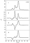 |
Fig. 1. Observed Stokes parameters (not corrected for instrumental polarization) I, V, Q, and U for o Ceti (in |

The data reduction was made with the CLASS5 package. The first step consists of removing linear baselines from all individual spectra. In a second step, we corrected the measured polarizations for the instrumental leakage from Stokes I to Q, U, and V; the method is described in Sect. 3.2. The third step consists of averaging under sensitivity-optimizing weighting all spectra for a given Stokes parameter to form a single spectrum that is to be analyzed.
From these, we computed the fractional circular polarization (pC), the fractional linear polarization (pL), and the angle of polarization (χ). These are defined as (Landi Degl’Innocenti & Landolfi 2004)
 (2)
(2)
The astronomical signal we obtained was an incoherent mixture of Stokes Q, U, and V parameters filling the observing beam, that is, originating from slightly different sight lines. The use of the four-quadrant inverse tangent function instead of the arctangent function avoids 90° ambiguities that arise when a significant polarization in Stokes U is measured together with an insignificant Stokes Q value of undefined sign. Owing to the modulation of Stokes Q and U in a noncorotating Nasmyth reference frame, this situation cannot be avoided and occurs frequently.
3.2. Instrumental polarization
Most astronomical telescopes and their instrumentation suffer from spurious conversions from Stokes I into Stokes Q, U, and V, and from conversions among the three latter parameters. The reasons for these conversions are manifold and mainly originate in the asymmetric optics of the telescope (e.g., Nasmyth designs such as that of the IRAM-30 m) and the reimaging system of the receivers and in the receiver feed horns. For a discussion, we refer to (Thum et al. 2008, and further references therein), who demonstrated the extremely low instrumental conversion of the IRAM-30 m optics from Stokes I into Stokes V (Müller matrix element MIV at the per-mil level even outside the optical axis after optimization of the orientation of the beam-splitting grid). In December 2015, the E090 band of EMIR was equipped with an ortho-mode transducer that splits the orthogonal linear polarizations only in the feed horn. Its imperfections induce an instrumental polarization of up to MIV = 2.7%, derived from observations of the unpolarized planet Uranus. Calibration of the polarization angle is as good as  , which is the uncertainty of the orientation of the wire grid in the phase-calibration unit. A spurious conversion from Stokes U to V may arise in the phase calibration, but is shown to fall below MUV ≲ 1%. From the Crab nebula observations performed at the beginning and end of each period, we derived a stable polarization angle of 145–146° that agrees with what is expected (Aumont et al. 2010; Ritacco et al. 2018). This demonstrates that the instrumental conversions between linear and circular polarization are under control. For brevity, we therefore use “instrumental polarization” as a synonym for the leakages from Stokes I into Q, U, and V, referring to specific conversions with the Müller matrix elements MIQ, MIU, and MIV. In the following, we describe the method for determining the instrumental polarization and for removing it from the Stokes spectra. It is important to note that these calibration steps were applied scan-wise, that is, to spectra of typically four-minute long on-off cycles. This is because the instrumental polarization arises predominantly in the Nasmyth cabin, and therefore, if it is expressed in celestial reference frames, it depends on elevation. The final spectra were subsequently obtained by averaging the calibrated scans.
3.2.1. Removal of instrumental leakage from Stokes I to Stokes V
A given Stokes V spectrum is composed of an astronomical signal, V⋆, and an instrumental leakage from Stokes I, that is, V = V⋆ + MIV ⋅ I. Our recovery of V⋆ proceeded as follows:
-
Since the MIV term is known to be quasi-achromatic, it can be quantified for each scan by the linear regression of Stokes I and V. By averaging only spectra with |MIV|< 1%, we obtained an almost pure preliminary astronomical Stokes V spectrum,
 .
. -
 was subtracted from each Stokes V spectrum. The resulting scan series of residual spectra ΔV was then largely dominated by the leakage terms MIV ⋅ I. Estimates of MIV were scan-wise determined by linear regression of Stokes I and ΔV.
 -
In the final step, we computed V⋆ = V − MIVI. The series of corrected spectra with baseline noise σrms obtained in this way were finally averaged with a sensitivity-optimizing
 weighting.
A demonstration of this algorithm is shown in Fig. A.1. The residual instrumental polarization in the cleaned Stokes V spectra mainly arises in the uncertainties ΔMIV of the parameters MIV obtained in this way and was estimated by applying the same calibration steps to synthetic Stokes V spectra of an underlying V⋆ known a priori. We list these steps below.
-
As data model for a given target, we used its
 spectrum produced by the rvm code (see Sect. 4.1). For each scan out of the total of Nobs observations, we added baseline noise of the standard deviation σrms and an instrumental contribution (MIV + ΔMIV)I. The Nobs realizations of the synthetic noise spectra and ΔMIV parameters were obtained from Gaussian distributions of the same standard deviations as were determined in the calibration steps described above.
 -
We decontaminated this set of Nobs simulated spectra and deduced the best estimate
 of the astronomical Stokes V spectrum using the same cleaning procedure as described above.
 -
We repeated this procedure ten times to obtain the standard deviation among the
 spectra for each velocity channel and assigned it to the corresponding channel of the
  spectrum.
For all sources, we applied this Monte Carlo method. We obtained standard deviations σV of about a few mK that we list in Table 2. They exceed those of the radiometric noise in the original Stokes V spectra and reflect the residual uncertainty in the determination of the MIV parameters. We underline that the previous test for the reproducibility of the required correction for R Aql indicates that the derived BZ × cos(θ2) is inconclusive. It is only formally significant that the  spectrum uncertainty is only based on the radiometric noise; no limitations are linked to the procedure for removing the MIV terms.
Global uncertainties (standard deviations) of Stokes V derived from the Monte Carlo method, including uncertainties in the removal of instrumental contamination.
3.2.2. Removal of instrumental leakage from Stokes I to Q and U
The removal of the leakage from Stokes I to linear polarization is conceptually easier because in the celestial reference frame (where the polarization angle is measured in the equatorial system from the north towards the east following the IAU convention, IAU 1973), the astronomical polarization explicitly depends on the parallactic rotation, or, to be more precise, on the difference χ0 between the telescope elevation ε and the parallactic angle η, whereas the instrumental contribution remains fixed in the reference frame of the Nasmyth cabin. For the EMIR receiver, the transformation from celestial coordinate offsets defined in the equatorial frame (Δα cos δ, Δδ) to those defined in the Nasmyth frame is given by
 (3)
(3)
The application of the coherency matrix formalism (e.g., Wiesemeyer et al. 2014, further references therein) then yields the corresponding transformation of the equatorial plane of the Poincaré sphere to the Nasmyth reference frame (subscript N), with the following representation of the Stokes Q and U parameters:
 (4)
(4)
where the superscripts * refer as in Sect. 3.2.1 to the astronomical Stokes parameters, and where MIQ and MIU are the Müller matrix elements for the spurious conversion of Stokes I into Q and U. The knowledge of the exact nature of the MIQ and MIU terms is not required here, except that their origin is located in the Nasmyth cabin, and that they are quasi-achromatic across the lines profiles here. From previous commissioning work (Thum et al. 2008), these prerequisites are known to be fulfilled. Under the well-justified premise that the emission in the Stokes parameters Q* and U* is spatially unresolved and stationary on the timescale of an hour-angle interval, and ensuring sufficient sampling of 2χ0, they can be separated from the instrumental contamination by fitting sinusoidal curves to the line-integrated fluxes using Eq. (4). An example is shown in Fig. A.2. Minor systematic deviations hint at another instrumental contribution to the measured polarization that is fixed in the horizontal system and therefore arises from the telescope’s primary or secondary mirror. These contributions were found to be insignificant.
4. Data analysis and method
4.1. Stokes I and V component analysis
The SiO Stokes I spectra are shown in Fig. 2 for R Aql and are presented in Appendix B (Fig. B.1) for the other sources. All SiO line profiles are complex, but can be reproduced by assembling several Gaussian maser components centered at different velocities. The individual components are relatively narrow, although some of them are slightly broader than the thermal line widths, about 1–1.2 km s−1 in SiO maser regions where we expect the gas temperature to be about 1000–1500 K. We decomposed the Stokes I signal into multiple Gaussian functions, assuming that the intensity profile I can be fitted by
 (5)
(5)
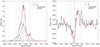 |
Fig. 2. Decomposition of Stokes I and V for R Aql (spectral resolution of 0.139 km s−1). Left: Stokes I data are shown in black, and the global fit is shown in red. The vertical dashed colored lines are the positions of the center of the individual Gaussian functions used in the fit, plotted in various colors. Right: Stokes V data cleaned from instrumental polarization are shown in black (Sect. 3.2), and the fit is shown in red. The vertical dashed colored lines show the individual Gaussian I components from the Stokes I fitting procedure (left panel). |
with v0, k and ΔvD, k the central velocity and Doppler width, respectively, for each component k, and Ak a weight coefficient.
We developed a code based on the relevance vector machines (rvm) algorithm as described in Tipping & Faul (2003). This code fits the signal to the best linear combination of entries taken from a dictionary. In our case, the dictionary was made of Gaussian functions of various widths (full width at half maximum, FWHM) that were chosen in a range of two values, Δva and Δvb, sampled in 50 values. They were defined for each star and centered over a range of velocities (200 values between v0 and v1). The term dictionary is used to emphasize that there is no requirement of orthogonality among the different elements of the dictionary. Lacking this requirement, the algebraic problem has no unique solution. rvm solves this issue by Bayesian marginalization. The code assigns a weight to all the components of the dictionary (Ak), optimizing the marginal likelihood. In a sense, the algorithm seeks the linear combination with the smallest number of dictionary entries that satisfies noise constraints, consistent with the noise observed in our data.
Initial fits were made with the CLASS package to obtain a first idea of the ranges for the widths and velocities. These parameters were then used as a first guess for the ranges in the rvm code. The ranges were adjusted iteratively to maximize the correlation between the fit and the observed spectra. The results are not sensitive to the adopted ranges when they remain within reasonable values. The FWHM ranges differ slightly for each source, but they are typically between 0.3 and 2 km s−1. The fit result is more sensitive to the noise level put in the algorithm, that is, the Stokes root mean square error (rms), which will constrain the number of components used in the fit.
Always assuming that circular polarization has its origin in the Zeeman effect, we used an analogous decomposition for the Stokes V profiles. Since SiO is a nonparamagnetic molecule, the typical magnetic fields expected to be found in the CSE correspond to the so-called weak-splitting Zeeman regime, for which the Zeeman splitting is much smaller than the intrinsic Doppler line width ΔvD. This is independent of any line width growing in the maser theory, but we describe the impact of maser saturation below. In the weak-field regime, any Stokes V signal can be safely modeled,
 (6)
(6)
where f(B) is a function of the magnetic field intensity and the parameters of the transition, with respect to the associated intensity. As in the case of the observed Stokes parameter I, the observed parameter V is broken down into subcomponents Vi that are derivative of Gaussian functions, which, when added together, fit the V profile. Our rvm algorithm determines the weights assigned to all Vi whose weighted combination fits the observed V. All profiles were treated here as would be done with thermal Zeeman measurements, but maser amplification may modify the line profiles (maser saturation is considered in Sect. 4.4).
The fit results for Stokes I and V are given in Tables 3–4 and are shown in Fig. 2 for R Aql and in Fig. B.1 (Stokes I) and 3 (Stokes V) for the other sources.
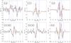 |
Fig. 3. Stokes V spectra for all sources except R Aql. The Stokes V data cleaned from instrumental polarization are shown in black (Sect. 3.2), and the fit is presented in red. The dashed purple lines are the positions of the individual Gaussian I components from Stokes I fitting procedure. |
Description of the I components for each source and the associated saturation rates.
4.2. Computation of the uncertainties
To compute the uncertainties δB of the inferred magnetic field, we computed the uncertainties δV of the Stokes V parameters after the removal of the instrumental polarization as described above. We considered two main sources of uncertainties:
-
The Monte Carlo method described in Sect. 3.2.1 includes the Stokes V global uncertainty for each velocity channel, that is, it reflects both the radiometric noise and the uncertainty in the removal of the MIV terms (see σV in Table 2). This entails an uncertainty δVinst in the rvm fit that needs to be quantified.
-
The second source of uncertainties is the difference (residual), δVres, between the fit and the cleaned spectra V⋆ (see Sect. 3.2.1).
We can quantify the first uncertainty from the standard deviations σV as determined in Sect. 3.2.1, which propagates into the parameters of the Stokes V fitting method and, consequently, to the magnetic field estimates. To determine this first uncertainty, we defined three spectra, namely the cleaning-method spectrum and two spectra deviating from the cleaned spectrum by ±σV. We applied the rvm code to these three spectra to determine whether there are differences in the parameters of the Gaussian functions (velocity widths, central velocities, and amplitudes) used in the fit. We find a difference of 0.3 km s−1 in the central velocity for U Her in May and 0.1 km s−1 for the three sources μ Cep, o Ceti, and U Her (March), while there is no difference for the other objects. We also determined the corresponding difference δVinst between the largest excursions introduced in the peak intensities Vpeak; it amounts to 7 mK.
To estimate δVres, we measured the rms error ( , with xm the fitted values and xd the observational data). For R Aql, μ Cep, and U Her (March observation), we find δVres ∼ 7 mK and for U Her (May observation), R Leo, Ceti, and χ Cyg 24, 28, 28, and 33 mK, respectively.
To obtain the total uncertainty δV in Stokes V, we added δVinst and δVres in quadrature; the results are reported in Table 4. Their high signal-to-noise ratios show that the Stokes I spectra are free from errors. For both regimes (i.e., saturated and unsaturated), the uncertainties in the magnetic field estimates are then given by δB/B = δV/V.
Characteristics of the Gauss-fit components to the observed Stokes V spectrum for each source.
4.3. Description of the observed Stokes I and V signals
Our fit results (see Figs. 2 for R Aql 3 for the V decomposition, B.1 for I, and Tables 3, 4) show that the SiO maser line profiles are globally well reproduced by our procedure. Exceptions can be found in the bluest and reddest weak features of the total intensity I, for instance, at ∼54 km s−1 for R Aql, but also for χ Cyg, o Ceti, or U Her (for the May data). Some broad wing emissions in μ Cep, χ Cyg, or o Ceti (including component 1) are not reproduced either. This has no impact on our results because the polarization of these components is weak and within the noise. The amplitudes of all detected Stokes I components are well above 10σ and are ∼1 km s−1 (or less) broad, as expected from maser emission (e.g. Richards et al. 2020). However, one central component in R Leo has a width of 2.3 km s−1, but this might be due to an underestimation (too weak) of the other components on both sides. We underline that the maser emission in U Her has changed between the two observation epochs. For this source, the profiles are different, although we identified the same number of components (five), but at different velocities. The last component at –10.4 km s−1 in March has no equivalence in May. The first components at –20.1 km s−1 (March) and –19.7 km s−1 (May) have the same intensity and width. Between the components at –17.7/–17.4 km s−1 and –16.0/–16.2 km s−1, which are weaker in May, the code found an additional larger (Δv = 1.3 km s−1), component at –17.0 km s−1 in May (see Fig. B.1).
Two types of V profiles are globally observed within our sample: single profiles with one to two well-separated Zeeman components (R Aql and U Her in May, and μ Cep) and more complex profiles with more components, some of them overlapping. U Her in March is between the two cases and does not exhibit the simple antisymmetric profile observed in May. It is important to note that not all I components are associated with characteristic antisymmetric Zeeman V profiles; the reason might be the complexity of the magnetic field within our rather large radio beam width. The Zeeman features in Stokes V that can be associated with a Stokes I component are (blue- or red-) shifted by a few 0.1 km s−1, and therefore, in general more than our uncertainty on the fits (see Sect. 4.2) and comparable to or exceeding the channel separation. This velocity shift is thus real, but we cannot explain it with a simple model associating physical maser components with emission peaks and a magnetic field. We cannot exclude based on our work that other theories without a standard Zeeman interpretation could lead to complex profiles with possible velocity shifts.
The V spectra for R Aql and U Her (May data) exhibit a well-defined single Zeeman signature that is redshifted from the corresponding I component. μ Cep exhibits two well-separated Zeeman signatures, also redshifted, but with a low S/N. The fit for U Her (March data) indicates three components, but considering the S/N, only the central one (in orange in Fig. 3), which is roughly identical to that detected in May, can be trusted. The V profiles for χ Cyg, R Leo, and o Ceti are made of five or six components each, most of them associated with I components, but with noticeable velocity shifts. o Ceti exhibits broad negative V signals in the bluest and reddest sides of the V profiles, which cannot be fit by Zeeman profiles. Extreme components in R Leo cannot be reproduced either.
We may speculate that μ Cep, U Her, and R Aql exhibit fewer V components because the SiO maser emission is weaker than that of the other objects, that is, the S/N is not sufficient to reveal other possible V components.
4.4. Maser line saturation
The cosmic maser line theory predicts an exponential growth of the line intensity until the population inversion reaches a critical saturation level, beyond which the radiated emission increases linearly along the propagation axis and tends to be beamed (see e.g. Goldreich & Kwan 1974). A convenient way to estimate whether the maser saturation conditions apply consists of comparing the stimulated emission rate of the maser transition, R, with the decay rate, Γ, from the maser levels. Saturation is observed when R exceeds Γ.
The stimulated emission rate is derived from
 (7)
(7)
where k and h are the Boltzmann and Planck constants, Tb is the brightness temperature, A = 2.891 × 10⁻⁵ s−1, the Einstein coefficient for spontaneous emission of transition SiO v = 1, J = 2 − 1, ν the line frequency, and ΔΩ the beaming solid angle (the ratio of the surface area of a typical maser spot to the area of the masing cloud).
Deriving R for the v = 1, J = 2 − 1 SiO transition depends critically on the estimate of ΔΩ and Tb. ΔΩ was estimated from the interferometric maps of SiO at 43 GHz in the v = 1, J = 1 − 0 transition observed in one typical Mira star over several epochs (Assaf et al. 2013); the average over all epochs is about 5 × 10⁻², but we note that the minimum and maximum beaming can vary from 2 × 10⁻² to nearly 0.1 at different epochs. We assumed that ΔΩ = 5 × 10⁻² is also representative of the beaming angle for the SiO v = 1, J = 2 − 1 transition. To estimate Tb in the absence of high spatial resolution maps of the observed sources, we relied on the existing measurements made in a broad variety of late-type stars. We adopted 1 au for the typical maser sizes, as in Pérez-Sánchez & Vlemmings (2013), and Tb then depends on the distance to the source and the observed total flux density. The estimated Tb is about 1–160 107 K (see Table 3, with two different values for two possible distances in R Aql and μ Cep), which strongly agrees with the maser nature of these emissions. The derived values of R are given in Table 3.
The decay rate from the maser levels may be approximately estimated without describing any pumping scheme when we recognize that collisional excitation of vibrational states followed by radiative decay is essential to explain the observed SiO masers in the v = 1 state and above (Elitzur 1992). At 86 GHz in the v = 1 state, we thus obtain an approximate value of Γ from the spontaneous emission rate A(v = 1 → 0) = 5 s−1 (Hedelund & Lambert 1972), which remains much higher than the collisional deexcitation rate, C(v = 1 − 0) a few times 10−3–10−4 s−1 for the temperature and density conditions expected in regions where SiO is observed. The density must remain below very roughly 1012 cm−3 to avoid collisional quenching of the SiO maser.
Despite the uncertainties on the values of R and Γ, we therefore obtained an estimate of the degree of saturation of the emitting maser for each intensity component and each star (see Table 3). Based on this, we propose which stars are in the unsaturated (R < Γ) or in the saturated cases (R > Γ). The result was used to prefer either one or the other of the theories described in Sect. 4.5 to compute the magnetic field.
Our results show that only χ Cyg, μ Cep (in the case of the larger distance), and U Her are saturated. Considering that we derived lower limits, however, we deemed these objects to be strongly saturated and the others to be just saturated. It is commonly admitted in the literature that circumstellar SiO masers are in the saturated or strongly saturated regime (e.g., Kemball et al. 2009). We still considered both cases for each star.
4.5. Magnetic field estimate
The computation of the magnetic field strength via the Zeeman effect differs according to the saturation of the maser emission. The magnetic field was computed from the two peaks found for Stokes V with our rvm code. With the Gaussian decompositions used in Eq. (5), the intensity extrema are observed at
 (8)
(8)
The two peaks, noted a and b (see Table 5), are separated by  (see Table 4).
Polarization rates, angles, and magnetic field values for all components and all stars for the saturated and unsaturated cases.
4.5.1. Saturated maser
In a saturated maser, the fractional Stokes vectors propagating through the masing cloud are constant. The radiative transfer equation for the Stokes vectors admits very few situations with a nonzero constant and propagating Stokes vector. These solutions were thoroughly studied by Elitzur (1996), while other theories were proposed (see Herpin et al. 2006, for a brief discussion).
We write the ratio xB of the Zeeman shift ΔvB to the Doppler line width ΔvD both in km s−1,
 (9)
(9)
for the Zeeman effect by explicitly writing ΔvB = 14gλ0B, where g is the Landé factor in terms of the Bohr magneton (where g for the diamagnetic molecule SiO is 8.44 × 10⁻⁵; see Appendix C), λ0 = 0.34785 cm the wavelength of the SiO v = 1 J = 2 − 1 maser emission, and B the magnetic field strength in Gauss.
Under the saturation regime and for the ratio xB < 1 (which is appropriate for diamagnetic molecular species), Elitzur (1996) found that xB is proportional to the fractional circular polarization pC at the peak of the Stokes V parameter according to the law
 (10)
(10)
where θ1 is the angle between the magnetic field direction and the incident beam arriving at the SiO molecule.
Herpin et al. (2006) followed a similar approach to estimate the magnetic field strength from their observed values of pC. However, they used g = 10−3, so that their field strength estimates must be reevaluated using g = 8.44 × 10⁻⁵ for comparison with our new study (see Sect. 6). From ΔvB above and Eq. (10) we obtain at the peak, vpeak, of the Stokes V parameter
 (11)
(11)
Equation (11) was used to derive the magnetic field strength in Gauss, noted BE in the following, when pC and ΔvD are known. The remaining uncertainty in the determination of the field intensity comes from θ1, which is discussed in Sect. 4.5.3.
4.5.2. Unsaturated maser
Whenever the maser is unsaturated and the fractional Stokes vectors are not constant along the optical path, the typical weak-field approximation applies. The Zeeman frequency shift of a given level is proportional to the Larmor frequency,
 (12)
(12)
where h is the Planck constant. The magneton μ often is the Bohr magneton. For the diamagnetic molecule SiO, however, all electronic angular momenta are zero and the only contribution to the total angular momenta comes from angular momenta associated with the rotation of the total mass of the molecule. These momenta are expressed in units of the nuclear magneton. It is common, however, to rewrite formulae in terms of the Bohr magneton and to redefine the Landé factor accordingly. The details can be found in Appendix C. We adopt this convention below, and as in the case of the saturated maser, we write all formulae in terms of the Bohr magneton.
Under the weak-field approximation, it can be demonstrated that the expected Stokes V line profile is proportional to the derivative of the intensity profile (see also Eq. (6)),
 (13)
(13)
where θ2 is the angle between the magnetic field direction and the emitted beam (toward the observer). We can express V as a function of B with the velocity axis sampled with a channel separation of 0.139 km s−1,
 (14)
(14)
Once again, we assumed that the line profile of each maser component is Gaussian, allowing us to retrieve the magnetic field strength from the peak amplitudes of Stokes V and I,
 (15)
(15)
dv being the derivative with respect to the velocity  .
.
In the unsaturated case, the magnetic field strength is noted BZ in the following.
4.5.3. Determining the angle of incidence of the maser beam
The two different angles, θ1 and θ2, defined earlier for the saturated and unsaturated cases, respectively, are hard to determine unless we have access to independent information about the field direction. As xB is lower than one, all Zeeman components overlap and only the type 0 polarization case described in Elitzur (1996) applies. Following Elitzur’s reasoning, we can compute angle θ1 in the saturated case using our linear polarization results.
Under the weak-field approximation, there is no linear polarization in the maser line (see review by Watson 2009). A second-order approximation can be proposed for linear polarization, but it does not describe the linear polarization profiles correctly. Linear polarization due to the Zeeman effect is one order of magnitude lower in general than circular polarization (Pérez-Sánchez & Vlemmings 2013) and has zero net polarization over wavelength (see Landi Degl’Innocenti & Landolfi 2004). It might be claimed that we observe the very specific geometries that afford large amplitudes to linear polarization under the Zeeman effect: fields transverse to the line of sight. It appears to be incongruous to accept that we systematically observed transverse fields, however. The Zeeman effect cannot produce Gaussian-like profiles under the weak field approximation for linear polarization such as those observed here (e.g. Wiebe & Watson 1998; Watson 2009). Faraday rotation6 can produce net linear polarization, but in order to do so, the magnetic fields involved would be too strong to be described under the weak-field approximation, and then, circular polarization cannot be explained in its amplitude nor in its shape. We can safely conclude that under the hypothesis of the weak-field approximation, the observed linear polarization must be due to another physical mechanism than the Zeeman effect, as we further discuss in Sect. 5.1. On the other hand, Elitzur’s theory shows that a linear polarization signal is to be expected together with the circular polarization one. Once more under the assumption of a Gaussian line profile and following (Elitzur 1996), in a coordinate system that is aligned with the sky-plane projected magnetic field, q = Q/I is given by
 (16)
(16)
with R1 a function of xB (defined in Eq. (9)) and of the dimensionless frequency argument x defined in Elitzur (1996). The numerical values of xb are low, and R1 is therefore not sensitive to the exact values of ΔvB and ΔvD. This is used below to derive the critical value of q when θ1 approaches 90° near the SiO line center where x = 0,
 (17)
(17)
The dependence of q on θ1 is shown in Fig. 4. Given our typical S/N ratios, and due to the quadratic dependence of B and the weak values of the field strength expected, the relation shown in this figure is independent of the field strength. A value of q provides us with an independent estimate of θ1.
 |
Fig. 4. Ratio q = Q/I vs. the angle θ1 (Eq. (16)). The green zone (|q|< qc) contains two solutions for the angle, as shown with the example with |q| = 0.25, the two green lines. Beyond this zone (example in blue), only one solution is possible. |
This linear polarization q is perpendicular to the plane that is formed by the incident beam direction and the magnetic field vector, and no other linear polarization signal is expected. We ignore what this direction is in any maser component, and we therefore ignored how this linear polarization is projected into our instrument directions for Stokes Q and Stokes U. The total measured polarization pL must be the total amplitude of the emitted linear polarization q in Elitzur’s theory, however, except for its sign. Since we only have access to the absolute value of pL from our observations, two different situations may occur depending on the measured value of pL with respect to a critical value qC defined by  ,
,
-
|q|> qc: The solution for the angle θ1 is unique (see the blue example in Fig. 4).
-
|q|< qc: There are two solutions for θ1 (see the green example), and hence, two solutions for the magnetic field strength.
5. Results
5.1. Observed polarization and maser excitation
The circular and linear polarization fractions derived for each identified V component in each star are given in Cols. 6 and 7 of Table 5 for each detected component. The other columns present the magnetic field estimates that are discussed in the next section.
Two regimes for the linear polarization are observed in our sample. μ Cep, R Aql, and U Her mostly exhibit low levels of the pL parameter (< 25%), while other stars show high pL values, up to 60%. Our polarization levels can be compared with those of Herpin et al. (2006). The linear polarization fractions are similar in these two works. However, while they measured an average absolute value of the circular polarization of 9% and 5% in Miras and semiregular variables, respectively, we have only 1.9% in our sample (composed of five Miras and the RSG μ Cep). We also note that several components in Herpin et al. have pC-values at about or lower than 2%. The lower polarization level observed in RSG (Herpin et al. 2006) is also confirmed in pL for μ Cep, but not in circular polarization because this star exhibits the highest pC fraction in our sample. A specific comparison can be made for R Leo and χ Cyg, which are observed in both studies, even though the Stokes I maser line profile has changed strongly between the two observation epochs. The linear polarization fraction reaches the same 30% and 40% level for R Leo and χ Cyg (with some higher values for some components). The circular polarization is definitely lower in our case (2.3% maximum, compared to 10–20%).
These values might shed light on the origin of the observed polarization in relation with the Zeeman effect or other effects. We can investigate the mechanisms that could produce the observed linear polarization fractions. In the case of isotropic pumping of the energy levels giving rise to maser emission (e.g. Nedoluha & Watson 1990) and for a moderately saturated maser, pL greater than 15%, up to 25%, can only be generated with peculiar angle configurations (an angle θ2 larger than 45°). Under anisotropic pumping conditions, much higher pL values can be achieved, but no high pC values can be generated (see Lankhaar & Vlemmings 2019). Non-Zeeman mechanisms may also lead to circular polarization. Asensio Ramos et al. (2005), considering the Hanle effect, showed that changes in the radiation anisotropy conditions can result in the rotation of the electric vector position angle (EVPA) and in the anisotropic pumping of a dichroic maser. Several variations of anisotropic pumping mechanisms (e.g. Western & Watson 1983; Wiebe & Watson 1998; Watson 2009) or anisotropic resonant scattering of a magnetized foreground SiO gas (Houde 2014) have been proposed for the non-Zeeman case as well. These non-Zeeman mechanisms have been ruled out in some specific environments, and on the basis of very high spatial resolution observations (VLBI) of the EVPA (see e.g. Kemball et al. 2009; Richter et al. 2016; Tobin et al. 2019). Several polarized maser theories have successfully been developed, but none can fully explain all the observed cases.
As indicated by Wiebe & Watson (1998), non-Zeeman mechanisms in unsaturated masers should lead to a proportional relation between pC and pL (as pC would be created from pL) with  . Herpin et al. (2006) found a linear function between the two polarizations, but with a large spread. Our sample does not reveal any correlation (see Fig. 5, except maybe for R Leo). The second condition (
 ) is not fulfilled either (see Table D.1), as was also observed by Richter et al. (2016) and Tobin et al. (2019), except for χ Cyg. Considering that the maser emission in this star is definitely saturated (see Table 3), we adopted the Zeeman scenario for the whole sample. Nevertheless, we note that a velocity gradient along the propagation path, but still consistent with coherent SiO maser amplification in some sources, could enhance pC and might even produce non-antisymmetric Stokes V spectra (Nedoluha & Watson 1994).
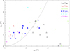 |
Fig. 5. Absolute fractional polarization pC vs. pL for the whole sample and all maser components. The dashed line corresponds to |

We considered the polarization angle χ as defined by Eq. (2). First, we underline that owing to our limited spatial resolution, the underlying Stokes Q and U parameters are beam-averaged quantities. Hence, if there were two spatially separated maser spots within our main beam, each one with a different EVPA, but emitting at the same velocity, we would not be able to interpret the measured χ angle rigorously. Only VLBI observations could separate two such maser spots and accurately trace the EVPA throughout the photosphere. As explained by Tobin et al. (2019), an angle between the maser propagation and the line of sight smaller or larger than the van Vleck angle (55°) will determine if the magnetic field is parallel or perpendicular to the EVPA, respectively. As in previous studies (e.g. Herpin et al. 2006; Kemball et al. 2011; Tobin et al. 2019), some χ jumps are observed for some sources across the SiO profile: R Leo (∼70° −160°), o Ceti (∼35° −70° −140°), and R Aql (∼95° −180°). The behavior in U Her is more erratic, that is, we do not observe beam-averaged π/2 jumps, while clear π/2 rotations are reported in VLBI publications. This can again be explained by beam-smearing effects in our data. A rotation like this together with the dependence of the fractional linear polarization on the angle between the magnetic field and the line of sight is predicted in linear and saturated masers that are isotropically pumped (Goldreich et al. 1973; Elitzur 2002). These models and the VLBI polarimetric observations of TX Cam (Kemball et al. 2011) tend to rule out the model proposed by Asensio Ramos et al. (2005), at least in this object. However, we also point out that although the Goldreich et al. (1973) maser model seems adequate, some Faraday rotation must be invoked to explain the smooth rotation of the EVPA (see Kemball et al. 2011; Tobin et al. 2019). Finally, we mention that changes in the EVPA could also result from rapidly changing magnetic field orientations above cool magnetic spots on the stellar photosphere (Soker 2002) (assuming that there are physical connections between photospheric spots and the upper atmospheric layers where SiO is observed).
5.2. Magnetic field strength
Applying the method described in Sect. 4.5, we derived estimates of the line-of-sight magnetic field strength BE and BZ × cos(θ2) for both the saturated and unsaturated cases for each star (see Table 5, Fig. 6, and Appendix D). As explained in Sect. 4.1, we computed the magnetic field strength at the two peaks of each detected antisymmetric V profile, which resulted in two extreme values of B for each Zeeman component (a and b in the Table 5). The values in the unsaturated case are higher in general.
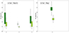 |
Fig. 6. Magnetic field values for U Her for the two observation periods, computed from Eq. (11) with two θ1 angle solutions, (dark and light green), when the linear polarization is below 33% (see Sect. 4.5.3 and Fig. 4). On the x-axis, the numbers correspond to the Gaussian components, as described in the second column of Table 5. The bar length corresponds to the difference between the magnetic field computed at the first and second peak of the derivative of the Gaussian component. |
While the angle θ2 in the unsaturated case remains unknown, in the saturated case, the angle θ1 was estimated, with two solutions at times when the linear polarization is lower than the critical value (see Sect. 4.5.3). This accordingly led to two possibilities for BE. These two solutions for the same angle θ1 were used to derive BE in Table 5. We cannot exclude that the observed linear polarization includes a contribution from non-Zeeman mechanisms, which would lead to some overestimation of pL, generated under the action of the Zeeman effect and hence of θ1. In this case, the BE values in Table 5 should be considered as lower limits.
At least two objects, χ Cyg and U Her, can be considered as giving rise to saturated masers (see Cols. 6 and 7 in Table 5). For χ Cyg, BE varies between 0.7 and 4.3 Gauss for components 1–5. We note that the results BZ × cos(θ2) for the unsaturated case are on the same order of magnitude (slightly higher for component 1). The results for component 6 are less reliable, considering the large uncertainty and difference in the estimate between the two peaks a and b (see Fig. D.1). We therefore excluded this component from the further discussion. For U Her, the magnetic field (BE) is about 0.9–1.5 Gauss in March and between 2.4–5.1 Gauss in May considering the central component 2, at a similar velocity for both periods. The other two side components (1 and 3) observed in March have large uncertainties and were not detected in May (see Fig. 6).
Considering that all other objects exhibit unsaturated maser emission (see Sect. 4.4), we assume that BZ × cos(θ2) provides a reliable estimate of the field, although θ2 remains unknown; indicative ad hoc values of θ2, for instance 45°, can be considered. Estimates of the magnetic field (assuming θ2 = 45°) differ from one star to the next and from one component to the next. In the case of R Aql, the Stokes V spectrum is largely dominated by the instrumental leakage of Stokes I into Stokes V (see Sect. 3.2.1). We therefore consider that BZ × cos(θ2) = 8.2 Gauss as given in Table 5 is an upper limit of the field intensity in the unsaturated case. For the two objects R Leo and o Ceti, the magnetic field in terms of the quantity BZ × cos(θ2) is 2.0–32.1 and 0.8–31.0 Gauss, respectively. Component 1 of o Ceti was discarded because we did not succeed in fitting this component with the derivative of a Gaussian function (see Sect. 4.3 and Fig. 3). Therefore, it may not be shaped by any Zeeman effect, in which case, the estimated magnetic field would not be relevant.
Because of the very low S/N for the V components in μ Cep (see Table 4), the field uncertainties are too large and are not taken into account in our discussion.
6. Discussion
Since the 1990s, various scenarios implying slow stellar rotation, the presence of a companion, and a weak magnetic field have been proposed to tentatively explain how the geometry of the CSE can be shaped in evolved stars (see for instance Soker & Harpaz 1992). All studies reported that the magnetic field strength is too weak to dominate the dynamics of the gas (Balick & Frank 2002; Herpin et al. 2006; Vlemmings et al. 2017). Nevertheless, a moderate field of about 1 Gauss at the stellar surface can play the role of a catalyst or a collimating agent (Soker 1998; Blackman et al. 2001; Greaves 2002). The role of a companion in shaping the envelope, without the need of invoking a magnetic field, has recently been demonstrated by Decin et al. (2020).
The strength of the magnetic field decreases with increasing distance r from the photosphere and can be expressed as a power law that depends on its geometry (Parker 1958; Matt et al. 2000; Meyer et al. 2021), in r−1, r−2, and r−3 for a toroidal, poloidal, and dipole field, respectively. When comparing their results to field estimates derived from the OH and H2O masers farther away in the CSE, Herpin et al. (2006), Duthu et al. (2017), and Vlemmings et al. (2017) concluded that a toroidal magnetic field was dominant (see also below). A combination of a toroidal and a poloidal field is nevertheless not excluded (see Meyer et al. 2021, for instance for RSGs).
In the following, we compare our newer observations and calculations to those in Herpin et al. (2006), who only considered saturated maser emission. First of all, we point out that the field intensities derived in Herpin et al. must be increased because an erroneous Landé factor (g = 10−3 instead of 8.44 × 10⁻⁵) and an erroneous wavelength were used; the corrective factor is 9.924. The magnetic field strengths derived here are thus lower than in Herpin et al. (2006) for the same circumstellar region where the SiO radio emission is observed (2–5 R⋆ from the photosphere, according to the SiO VLBI map). Herpin et al. (2006) found a mean value of ∼34 Gauss (which includes the corrective factor above), while our current estimates are below 32 Gauss (excluding the unreliable results in Table 5), and they show a mean value of 2.5 Gauss for the saturated case and 12.4 Gauss for the unsaturated one, assuming θ2 = 45°. When we only consider, as in Herpin et al. (2006), the saturated case, our magnetic field estimates range from 0.3 to 8.9 Gauss. We now focus the comparison on χ Cyg and R Leo, which were observed in both studies. While for R Leo (adopting θ1 = 45°), B was estimated by Herpin et al. (2006) to be 41–45 Gauss in the saturated case after reevaluation, we find somewhat lower values here: BE ∼ 0.3 − 8.5 G and BZ ∼ 2.8 − 4 G (at θ2 = 45° for the 2.0–32.1 G interval in Table 5) for the saturated and unsaturated cases, respectively. The two observations are separated by more than 20 yr, and not only the stellar activity, but also the magnetic field may have changed during this period. This holds for all objects. We nevertheless stress that despite uncertainties in the degree of maser saturation (resulting in an uncertainty on the B-formula), our careful calibration method and the Zeeman-component fitting procedure lead to reasonable magnetic field estimates. The case of χ Cyg is also illustrative. The field (BE) is 0.7–4.3 Gauss, which is to be compared with the former estimate from Herpin et al. (2006) of 48.6 Gauss (0–85.4 Gauss, after reevaluation of the field intensity). Considering the 2–3 Gauss measurement by Lèbre et al. (2014) at the surface of χ Cyg, we could expect a field strength of 0.5–1.5 or 0.1–0.8 Gauss in the SiO layer if the field varied as 1/r or 1/r2, respectively. Our results hence agree with a poloidal field, but do not rule out a toroidal component either, at least locally. This comparison has to be taken with caution, considering again that both measurements are well separated in time. The field strength variation observed in U Her over a two-month period emphasizes this point. In addition, for the RSG μ Cep, we derived higher upper magnetic field values than estimated by Tessore et al. (2017) at the stellar surface (1 Gauss). The fact that these two values are not compatible with a field strength that decreases with increasing distance may again underline the time variability of the magnetic field.
We revisit in Fig. 7 all magnetic field measurements from the literature. Our new measurements provide new constraints for the SiO shell region at a few stellar radii and appear to exclude a global poloidal field, especially when we assume that all maser emissions are saturated. Nevertheless, based on our χ Cyg observations, we cannot exclude a poloidal field close to the surface of this star that evolves into a dominant toroidal field in the SiO maser region, as proposed by Meyer et al. (2021) in supergiant stars.
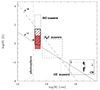 |
Fig. 7. Evolution of the field strength with distance (adapted from Vlemmings 2012; Duthu et al. 2017). The four boxes show the SiO masers (the red box represents the results of this work for a saturated maser, the hatched box for an unsaturated maser using θ2 = 45°, the dotted box the results from Herpin et al. 2006), the H2O and OH masers, and CN. The r−2 solar-type and r−1 toroidal magnetic fields are discussed in Sect. 6. The star close to the SiO maser box is for the magnetic field measured by Lèbre et al. (2014) in χ Cyg. The vertical dashed line indicates the stellar surface for the Miras. |
The origin of this magnetic field is still debated, but mechanisms involving an α2 − ω turbulent dynamo in AGB stars and amplification by convection, stellar pulsation, and cool spots can be invoked (Lèbre et al. 2014). As already proposed by Schwarzschild (1975) for giant stars, the radial component of the field can then be strongly enhanced at a specific location near the surface above cool magnetic spots (Priest 1987). The tangential B field component can be amplified by shock compression due to the stellar pulsation (Hartquist & Dyson 1997). A magnetic field of 1–10 Gauss can therefore be reached in the vicinity of cool magnetic spots, then decreasing in intensity to the 1/r2 law (Soker 2002). The same scenario applies in RSG stars with a stronger influence of their larger convective elements. As explained in Sect. 5.1, even the EVPA rotation seen in SiO features could be explained by a magnetic field orientation that changes rapidly above cool spots.
The magnetic field variations observed in the AGB U Her over a two-month scale (stellar phases 0.25 and 0.45) suggest a possible link with the stellar phase, that is, with pulsation and photospheric activity. It is interesting to note that for U Her, Baudry et al. (2023) also identified and mapped strong time variations of the 268 GHz v2 = 2 line of water at phases 0.13, 0.80, and 0.92 based on ALMA data. This line is excited in regions of the inner CSE where the SiO masers are observed. We also mention that (Rosales-Guzmán et al. 2023) have seen structural changes at 3 R⋆ in the CSE of the Mira R Car (period = 310 days) on a one-month interval in GRAVITY/VLTI data, which are probably linked to the photospheric activity. Quasi-simultaneous observations of the stellar photosphere (to detect cool spots) and polarimetry (to measure the field strength) are needed to prove any potential link. Polarimetric interferometric observations with ALMA or the next-generation VLA would ideally allow us to spatially associate stellar spots with B-field enhanced regions. The role of pulsation could also be studied with a monitoring of the magnetic field with stellar phase.
7. Conclusions
We have performed new polarimetric SiO maser observations with the XPOL instrument at the IRAM-30 m in a new sample of cool evolved stars. Applying a new data reduction method, we have removed most of the instrumental polarization to derive circular and linear polarization fractions with high accuracy. From these and maser theory results, we obtained magnetic field strengths (ranging from a few Gauss up to several dozen Gauss) that better constrain the SiO shell region above the stellar photosphere. A global poloidal field can be excluded.
Moreover, our observations of the magnetic field strength in U Her over a two-month period suggest a possible link with the stellar phase, that is, with pulsation/photospheric activity.
Despite the advances accomplished here, the precise origin of the observed magnetic field at the surface and in the inner circumstellar layers of AGB and RSG stars still remains to be fully characterized. In particular, a monitoring of the magnetic field to determine the stellar phase dependence of the polarization and quasi-simultaneous observations with VLTI and/or CHARA to detect cool spots and to follow the photospheric activity is under consideration. In addition, because our results still suffer from moderate spatial resolution, ALMA polarimetric observations above the photosphere would also be most desirable.
Echelle SpectroPolarimetric Device for the Observation of Stars.
We mean in-source Faraday rotation that modifies the radio polarization properties in the presence of a magnetic field. Electrons mixed up with the SiO cloud and in the circumstellar envelope could rotate the SiO linearly polarized wave; the latter effect is hopefully small given the short distances involved, unless the field intensity is strong.
Acknowledgments
This work is funded by the French National Research Agency (ANR) project PEPPER (ANR-20-CE31-0002). M.M. acknowledges funding from the Programme Paris Région fellowship supported by the Région Ile-de-France. This project has received funding from the European Union’s Horizon 2020 research and innovation program under the Marie Skłodowska-Curie Grant agreement No. 945298. We would like to thank IRAM staff at Granada (Spain) for their support. We also thank the referee for his careful reading and his useful comments and suggestions.
References
- Andriantsaralaza, M., Ramstedt, S., Vlemmings, W. H. T., & De Beck, E. 2022, A&A, 667, A74 [NASA ADS] [CrossRef] [EDP Sciences] [Google Scholar]
- Asensio Ramos, A., Landi Degl’Innocenti, E., & Trujillo Bueno, J. 2005, ApJ, 625, 985 [NASA ADS] [CrossRef] [Google Scholar]
- Assaf, K. A., Diamond, P. J., Richards, A. M. S., & Gray, M. D. 2013, MNRAS, 431, 1077 [NASA ADS] [CrossRef] [Google Scholar]
- Aumont, J., Conversi, L., Thum, C., et al. 2010, A&A, 514, A70 [NASA ADS] [CrossRef] [EDP Sciences] [Google Scholar]
- Aurière, M., Donati, J. F., Konstantinova-Antova, R., et al. 2010, A&A, 516, L2 [NASA ADS] [CrossRef] [EDP Sciences] [Google Scholar]
- Balick, B., & Frank, A. 2002, ARA&A, 40, 439 [Google Scholar]
- Baudry, A., Wong, K. T., Etoka, S., et al. 2023, A&A, 674, A125 [NASA ADS] [CrossRef] [EDP Sciences] [Google Scholar]
- Blackman, E. G., Frank, A., & Welch, C. 2001, ApJ, 546, 288 [NASA ADS] [CrossRef] [Google Scholar]
- Bladh, S., & Höfner, S. 2012, A&A, 546, A76 [NASA ADS] [CrossRef] [EDP Sciences] [Google Scholar]
- Bouvier, J. 2009, in EAS Publications Series, eds. C. Neiner, & J. P. Zahn, EAS Publ. Ser., 39, 199 [NASA ADS] [CrossRef] [EDP Sciences] [Google Scholar]
- Charbonnel, C., Decressin, T., Lagarde, N., et al. 2017, A&A, 605, A102 [NASA ADS] [CrossRef] [EDP Sciences] [Google Scholar]
- Cotton, W. D., Vlemmings, W., Mennesson, B., et al. 2006, A&A, 456, 339 [NASA ADS] [CrossRef] [EDP Sciences] [Google Scholar]
- Cotton, W. D., Ragland, S., & Danchi, W. C. 2011, ApJ, 736, 96 [NASA ADS] [CrossRef] [Google Scholar]
- Cranmer, S. R., & Saar, S. H. 2011, ApJ, 741, 54 [Google Scholar]
- Davis, R. E., & Muenter, J. S. 1974, J. Chem. Phys., 61, 2940 [NASA ADS] [CrossRef] [Google Scholar]
- De Beck, E., Decin, L., de Koter, A., et al. 2010, A&A, 523, A18 [NASA ADS] [CrossRef] [EDP Sciences] [Google Scholar]
- Decin, L., Richards, A. M. S., Danilovich, T., Homan, W., & Nuth, J. A. 2018, A&A, 615, A28 [NASA ADS] [CrossRef] [EDP Sciences] [Google Scholar]
- Decin, L., Montargès, M., Richards, A. M. S., et al. 2020, Science, 369, 1497 [Google Scholar]
- Dorch, S. B. F. 2004, A&A, 423, 1101 [NASA ADS] [CrossRef] [EDP Sciences] [Google Scholar]
- Duthu, A., Herpin, F., Wiesemeyer, H., et al. 2017, A&A, 604, A12 [NASA ADS] [CrossRef] [EDP Sciences] [Google Scholar]
- Ekström, S., Georgy, C., Eggenberger, P., et al. 2012, A&A, 537, A146 [Google Scholar]
- Elitzur, M. 1992, ARA&A, 30, 75 [NASA ADS] [CrossRef] [Google Scholar]
- Elitzur, M. 1996, ApJ, 457, 415 [NASA ADS] [CrossRef] [Google Scholar]
- Elitzur, M. 2002, in Astrophysical Spectropolarimetry, eds. J. Trujillo-Bueno, F. Moreno-Insertis, & F. Sánchez (Cambridge, UK: Cambridge University Press), 225 [Google Scholar]
- Freytag, B., Steffen, M., & Dorch, B. 2002, Astron. Nachr., 323, 213 [Google Scholar]
- Georgiev, S., Lébre, A., Josselin, E., et al. 2023, MNRAS, 522, 3861 [NASA ADS] [CrossRef] [Google Scholar]
- Goldreich, P., & Kwan, J. 1974, ApJ, 190, 27 [NASA ADS] [CrossRef] [Google Scholar]
- Goldreich, P., Keeley, D. A., & Kwan, J. Y. 1973, ApJ, 179, 111 [NASA ADS] [CrossRef] [Google Scholar]
- Gottlieb, C. A., Decin, L., Richards, A. M. S., et al. 2022, A&A, 660, A94 [CrossRef] [EDP Sciences] [Google Scholar]
- Greaves, J. S. 2002, A&A, 392, L1 [NASA ADS] [CrossRef] [EDP Sciences] [Google Scholar]
- Greve, A., Panis, J. F., & Thum, C. 1996, A&AS, 115, 379 [Google Scholar]
- Hartquist, T. W., & Dyson, J. E. 1997, A&A, 319, 589 [NASA ADS] [Google Scholar]
- Hedelund, J., & Lambert, D. L. 1972, Astrophys. Lett., 11, 71 [NASA ADS] [Google Scholar]
- Herpin, F., Baudry, A., Thum, C., Morris, D., & Wiesemeyer, H. 2006, A&A, 450, 667 [NASA ADS] [CrossRef] [EDP Sciences] [Google Scholar]
- Herwig, F. 2005, ARA&A, 43, 435 [NASA ADS] [CrossRef] [Google Scholar]
- Höfner, S., & Olofsson, H. 2018, A&ARv, 26, 1 [Google Scholar]
- Honerjäger, R., & Tischer, R. 1974, Z. Naturforsch. A, 29, 1695 [CrossRef] [Google Scholar]
- Houde, M. 2014, ApJ, 795, 27 [NASA ADS] [CrossRef] [Google Scholar]
- IAU 1973, Trans. Int. Astron. Union, 15, 165 [CrossRef] [Google Scholar]
- Josselin, E., Lambert, J., Aurière, M., Petit, P., & Ryde, N. 2015, in Polarimetry, eds. K. N. Nagendra, S. Bagnulo, R. Centeno, & M. Jesús Martínez González, 305, 299 [NASA ADS] [Google Scholar]
- Kemball, A. J., & Diamond, P. J. 1997, ApJ, 481, L111 [NASA ADS] [CrossRef] [Google Scholar]
- Kemball, A. J., Diamond, P. J., Gonidakis, I., et al. 2009, ApJ, 698, 1721 [NASA ADS] [CrossRef] [Google Scholar]
- Kemball, A. J., Diamond, P. J., Richter, L., Gonidakis, I., & Xue, R. 2011, ApJ, 743, 69 [NASA ADS] [CrossRef] [Google Scholar]
- Konstantinova-Antova, R., Aurière, M., Charbonnel, C., et al. 2014, in Magnetic Fields throughout Stellar Evolution, eds. P. Petit, M. Jardine, & H. C. Spruit, 302, 373 [NASA ADS] [Google Scholar]
- Landi Degl’Innocenti, E., & Landolfi, M. 2004, in Polarization in Spectral Lines, (Springer), Astrophys. Space Sci. Lib., 307 [Google Scholar]
- Langer, N. 2012, ARA&A, 50, 107 [CrossRef] [Google Scholar]
- Lankhaar, B., & Vlemmings, W. 2019, A&A, 628, A14 [NASA ADS] [CrossRef] [EDP Sciences] [Google Scholar]
- Lèbre, A., Aurière, M., Fabas, N., et al. 2014, A&A, 561, A85 [NASA ADS] [CrossRef] [EDP Sciences] [Google Scholar]
- Lèbre, A., Aurière, M., Fabas, N., et al. 2015, in Polarimetry, eds. K. N. Nagendra, S. Bagnulo, R. Centeno, & M. Jesús Martínez González, 305, 47 [Google Scholar]
- López Ariste, A., Tessore, B., Carlín, E. S., et al. 2019, A&A, 632, A30 [NASA ADS] [CrossRef] [EDP Sciences] [Google Scholar]
- Lucas, R., Bujarrabal, V., Guilloteau, S., et al. 1992, A&A, 262, 491 [NASA ADS] [Google Scholar]
- Maercker, M., Khouri, T., Mecina, M., & De Beck, E. 2022, A&A, 663, A64 [NASA ADS] [CrossRef] [EDP Sciences] [Google Scholar]
- Mathias, P., Aurière, M., López Ariste, A., et al. 2018, A&A, 615, A116 [NASA ADS] [CrossRef] [EDP Sciences] [Google Scholar]
- Matt, S., Balick, B., Winglee, R., & Goodson, A. 2000, ApJ, 545, 965 [CrossRef] [Google Scholar]
- Meyer, D. M. A., Mignone, A., Petrov, M., et al. 2021, MNRAS, 506, 5170 [NASA ADS] [CrossRef] [Google Scholar]
- Montargès, M., Homan, W., Keller, D., et al. 2019, MNRAS, 485, 2417 [CrossRef] [Google Scholar]
- Montargès, M., Cannon, E., Lagadec, E., et al. 2021, Nature, 594, 365 [Google Scholar]
- Nedoluha, G. E., & Watson, W. D. 1990, ApJ, 354, 660 [NASA ADS] [CrossRef] [Google Scholar]
- Nedoluha, G. E., & Watson, W. D. 1994, ApJ, 423, 394 [NASA ADS] [CrossRef] [Google Scholar]
- Parker, E. N. 1958, ApJ, 128, 664 [Google Scholar]
- Pascoli, G., & Lahoche, L. 2008, PASP, 120, 1267 [Google Scholar]
- Pérez-Sánchez, A. F., & Vlemmings, W. H. T. 2013, A&A, 551, A15 [NASA ADS] [CrossRef] [EDP Sciences] [Google Scholar]
- Priest, E. R. 1987, Solar Magneto-hydrodynamics (Dordrecht: D. Reidel) [Google Scholar]
- Richards, A. M. S., Sobolev, A., Baudry, A., et al. 2020, Adv. Space Res., 65, 780 [NASA ADS] [CrossRef] [Google Scholar]
- Richter, L., Kemball, A., & Jonas, J. 2016, MNRAS, 461, 2309 [NASA ADS] [CrossRef] [Google Scholar]
- Ritacco, A., Macías-Pérez, J. F., Ponthieu, N., et al. 2018, A&A, 616, A35 [NASA ADS] [CrossRef] [EDP Sciences] [Google Scholar]
- Rosales-Guzmán, A., Sanchez-Bermudez, J., Paladini, C., et al. 2023, A&A, 674, A62 [NASA ADS] [CrossRef] [EDP Sciences] [Google Scholar]
- Rudnitski, G. M., Pashchenko, M. I., & Colom, P. 2010, Astron. Rep., 54, 400 [NASA ADS] [CrossRef] [Google Scholar]
- Sabin, L., Wade, G. A., & Lébre, A. 2014, MNRAS, 446, 1988 [Google Scholar]
- Sahai, R., & Bieging, J. H. 1993, AJ, 105, 595 [NASA ADS] [CrossRef] [Google Scholar]
- Schwarzschild, M. 1975, ApJ, 195, 137 [NASA ADS] [CrossRef] [Google Scholar]
- Soker, N. 1998, MNRAS, 299, 1242 [NASA ADS] [CrossRef] [Google Scholar]
- Soker, N. 2002, MNRAS, 336, 826 [NASA ADS] [CrossRef] [Google Scholar]
- Soker, N., & Harpaz, A. 1992, PASP, 104, 923 [NASA ADS] [CrossRef] [Google Scholar]
- Tessore, B., Lèbre, A., Morin, J., et al. 2017, A&A, 603, A129 [NASA ADS] [CrossRef] [EDP Sciences] [Google Scholar]
- Thum, C., Wiesemeyer, H., Paubert, G., Navarro, S., & Morris, D. 2008, PASP, 120, 777 [NASA ADS] [CrossRef] [Google Scholar]
- Tipping, M. E., & Faul, A. C. 2003, in Proceedings of the Ninth International Workshop on Artificial Intelligence and Statistics, eds. C. M. Bishop, & B. J. Frey, PMLR, R4, 276, reissued by PMLR on 01 April 2021 [Google Scholar]
- Tobin, T. L., Kemball, A. J., & Gray, M. D. 2019, ApJ, 871, 189 [NASA ADS] [CrossRef] [Google Scholar]
- Vlemmings, W. H. T. 2011, in Asymmetric Planetary Nebulae 5 Conference, eds. A. A. Zijlstra, F. Lykou, I. McDonald, & E. Lagadec, 89 [Google Scholar]
- Vlemmings, W. H. T. 2012, in Cosmic Masers – From OH to H0, eds. R. S. Booth, W. H. T. Vlemmings, & E. M. L. Humphreys, 287, 31 [Google Scholar]
- Vlemmings, W. H. T., Khouri, T., Martí-Vidal, I., et al. 2017, A&A, 603, A92 [NASA ADS] [CrossRef] [EDP Sciences] [Google Scholar]
- Watson, W. D. 2009, Rev. Mex. Astron. Astrofis. Conf. Ser., 36, 113 [NASA ADS] [Google Scholar]
- Western, L. R., & Watson, W. D. 1983, ApJ, 275, 195 [NASA ADS] [CrossRef] [Google Scholar]
- Wiebe, D. S., & Watson, W. D. 1998, ApJ, 503, L71 [NASA ADS] [CrossRef] [Google Scholar]
- Wiesemeyer, H., Hezareh, T., Kreysa, E., et al. 2014, PASP, 126, 1027 [NASA ADS] [CrossRef] [Google Scholar]
- Wittkowski, M., Boboltz, D. A., Ohnaka, K., Driebe, T., & Scholz, M. 2007, A&A, 470, 191 [NASA ADS] [CrossRef] [EDP Sciences] [Google Scholar]
Appendix A: Removal of instrumental polarization
The removal of the instrumental leakage from Stokes I to Stokes V, as described in Sect. 3.2.1, is demonstrated for R Leo in the three panels of Fig. A.1. The final cleaned V spectrum (bottom panel) can be compared to the same V spectrum before cleaning (see Fig. 1). In Fig. A.2, we demonstrate the separation of the astronomical linear polarization from instrumental contributions again for the example of R Leo by fitting sine-waves, offset by the instrumental polarizations, to the fractional Stokes parameters QN/I and UN/I (as defined in the Nasmyth system, i.e., with respect to the receiver cabin; see Sect. 3.2.2), plotted against the angle χ0.
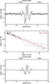 |
Fig. A.1. Illustration of our method to remove the instrumental polarization in Stokes V spectra for R Leo. Top: Average of Stokes V spectra with low leakage (|MIV|< 0.01). Center: Example of the correlation between Vinstr = MIV ⋅ I and Stokes I. The regression slope is MIV = −0.0271. Bottom: Final cleaned and averaged Stokes V spectrum. The vertical plot scale is the same as for the spectrum shown above. |
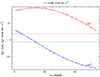 |
Fig. A.2. Separation of the astronomical linear polarization from instrumental contributions for the example of R Leo. The solid red and blue lines show least-squares fits to the fractional Stokes parameters QN/I and UN/I (red and blue dots, respectively) of R Leo vs. χ0 = ε − η, averaged across a velocity interval framing the Stokes I emission peak (0.68 to 2.04 km s−1) and expressed in the Nasmyth reference frame. The dashed lines indicate the corresponding fractional instrumental contributions. For details, see text. |
Appendix B: Stokes I spectra
Fig. B.1 presents the decomposition of Stokes I for μ Cep, o Ceti, χ Cyg, U Her (March and May 2022), and R Leo. The decomposition in R Aql is presented in Fig. 2 (left panel).
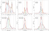 |
Fig. B.1. Fit results of the decomposition of Stokes I signal into multiple Gaussian functions as derived by the rvm code for μ Cep, o Ceti, χ Cyg, U Her, and R Leo (for R Aql, see Fig.2). |
Appendix C: Landé factors of the SiO maser lines.
In this appendix, we recall some basic notions that are used to describe the Zeeman effect in molecules and define the appropriate value of the Landé factor, g, to be used in the SiO transition observed in this work.
The Larmor frequency can be used to describe the Zeeman shift of a level (in the energy domain) or a Zeeman transition (in the frequency domain) up to a gyromagnetic factor called the Landé factor. This factor is not explicitly dependent on the angular momenta, which can be of two types. Those involving the electron produce an effect proportional to the Bohr magneton, which in SI units is given by

and those involving the whole molecule for which the nuclear magneton is relevant,

Both magnetons are related by the proton-to-electron mass ratio mp/me = 1836.
The molecule under study here, SiO, is diamagnetic (its ground electronic state is 1Σ+), and consequently, all its electronic angular momenta are zero. The Larmor frequency in terms of the nuclear magneton must be used,
![Mathematical equation: $$ \nu _L=\frac{\mu _N}{h}B=762.31 \cdot B[G] $$](/articles/aa/full_html/2024/08/aa49014-23/aa49014-23-eq37.gif)
(for reference, we recall the common Larmor frequency in terms of the Bohr magneton νL = 1.3996 × 10⁶ ⋅ B[G]).
Calling Zeeman shift the shift of an energy level with respect to its zero-field position, we define the Zeeman splitting as the separation between two usually symmetric Zeeman split components using the selection rule ΔMJ = ±1 or 0, where MJ is the projection of momentum J along the magnetic field axis (excluding 0 to 0 for ΔJ = 0). Laboratory measurements (Davis & Muenter 1974; Honerjäger & Tischer 1974) are coincident in assigning g ≈ 0.155 for all J rotational transitions of SiO in the first vibrational state v = 1. The Landé factor is slightly different, 0.154 in the v = 0 state (not observed here). (There is also a weak energy term that depends on the magnetic field due to the magnetic susceptibility anisotropy of the SiO molecule (Davis & Muenter 1974); it can numerically be ignored here.) The Zeeman shift of the v = 1 SiO transitions, in terms of the nuclear magneton, is thus gνL = 118.16 ⋅ B[G] and the Zeeman splitting is twice that value.
We have defined an explicit Landé factor including the appropriate correction from the Bohr magneton to the nuclear magneton as
We note that this was also used in Elitzur (1996) (see his dimensionless equation 1.1, where the Landé factor must account for the 1/1836 factor for diamagnetic molecules, however. Elitzur’s Doppler width is also half the total Doppler line width at half intensity), and also used in Kemball & Diamond (1997), Kemball et al. (2009) or in Asensio Ramos et al. (2005).
In this work, the Zeeman frequency is just twice the Zeeman shift, i.e.

For the SiO lines of interest, we have in Hz
![Mathematical equation: $$ g\Omega = 1524.6gB[G] $$](/articles/aa/full_html/2024/08/aa49014-23/aa49014-23-eq40.gif) .
.
Appendix D: Magnetic field strength
Fig. D.1 presents the magnetic field strengths of χ Cyg using Eq. 11 for saturated masers with two solutions when the linear polarization is lower than 33%. Figure D.2 presents the magnetic field strengths for R Leo and o Ceti for saturated masers from Eq. 11 (left panel) and for unsaturated maser from Eq. 15 (right panel). Table D.1 shows the average circular polarization fraction  and average
  for each star.
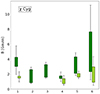 |
Fig. D.1. Magnetic field values for χ Cyg, with two θ1 angle solutions, (dark and light green), when the linear polarization is below 33%). On the x-axis, the numbers correspond to the Gaussian components, as described in the second column of Table 5. The bar length corresponds to the difference between the magnetic field computed at the first and second peak of the derivative of the Gaussian component. |
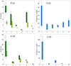 |
Fig. D.2. Magnetic field estimates considering both cases, saturated and unsaturated, for R Leo and o Ceti, objects for which we couldn’t determine their saturation status. The magnetic field computed with the Elitzur formula is shown in green (Left). The magnetic field from the Zeeman weak-field theory (B × cos(θ2)) is shown in blue (Right). |
Average circular polarization fraction  and average
  for each star.
All Tables
Global uncertainties (standard deviations) of Stokes V derived from the Monte Carlo method, including uncertainties in the removal of instrumental contamination.
Description of the I components for each source and the associated saturation rates.
Characteristics of the Gauss-fit components to the observed Stokes V spectrum for each source.
Polarization rates, angles, and magnetic field values for all components and all stars for the saturated and unsaturated cases.
All Figures
|
Fig. 1. Observed Stokes parameters (not corrected for instrumental polarization) I, V, Q, and U for o Ceti (in |
| In the text | |
|
Fig. 2. Decomposition of Stokes I and V for R Aql (spectral resolution of 0.139 km s−1). Left: Stokes I data are shown in black, and the global fit is shown in red. The vertical dashed colored lines are the positions of the center of the individual Gaussian functions used in the fit, plotted in various colors. Right: Stokes V data cleaned from instrumental polarization are shown in black (Sect. 3.2), and the fit is shown in red. The vertical dashed colored lines show the individual Gaussian I components from the Stokes I fitting procedure (left panel). |
| In the text | |
|
Fig. 3. Stokes V spectra for all sources except R Aql. The Stokes V data cleaned from instrumental polarization are shown in black (Sect. 3.2), and the fit is presented in red. The dashed purple lines are the positions of the individual Gaussian I components from Stokes I fitting procedure. |
| In the text | |
|
Fig. 4. Ratio q = Q/I vs. the angle θ1 (Eq. (16)). The green zone (|q|< qc) contains two solutions for the angle, as shown with the example with |q| = 0.25, the two green lines. Beyond this zone (example in blue), only one solution is possible. |
| In the text | |
|
Fig. 5. Absolute fractional polarization pC vs. pL for the whole sample and all maser components. The dashed line corresponds to |
| In the text | |
|
Fig. 6. Magnetic field values for U Her for the two observation periods, computed from Eq. (11) with two θ1 angle solutions, (dark and light green), when the linear polarization is below 33% (see Sect. 4.5.3 and Fig. 4). On the x-axis, the numbers correspond to the Gaussian components, as described in the second column of Table 5. The bar length corresponds to the difference between the magnetic field computed at the first and second peak of the derivative of the Gaussian component. |
| In the text | |
|
Fig. 7. Evolution of the field strength with distance (adapted from Vlemmings 2012; Duthu et al. 2017). The four boxes show the SiO masers (the red box represents the results of this work for a saturated maser, the hatched box for an unsaturated maser using θ2 = 45°, the dotted box the results from Herpin et al. 2006), the H2O and OH masers, and CN. The r−2 solar-type and r−1 toroidal magnetic fields are discussed in Sect. 6. The star close to the SiO maser box is for the magnetic field measured by Lèbre et al. (2014) in χ Cyg. The vertical dashed line indicates the stellar surface for the Miras. |
| In the text | |
|
Fig. A.1. Illustration of our method to remove the instrumental polarization in Stokes V spectra for R Leo. Top: Average of Stokes V spectra with low leakage (|MIV|< 0.01). Center: Example of the correlation between Vinstr = MIV ⋅ I and Stokes I. The regression slope is MIV = −0.0271. Bottom: Final cleaned and averaged Stokes V spectrum. The vertical plot scale is the same as for the spectrum shown above. |
| In the text | |
|
Fig. A.2. Separation of the astronomical linear polarization from instrumental contributions for the example of R Leo. The solid red and blue lines show least-squares fits to the fractional Stokes parameters QN/I and UN/I (red and blue dots, respectively) of R Leo vs. χ0 = ε − η, averaged across a velocity interval framing the Stokes I emission peak (0.68 to 2.04 km s−1) and expressed in the Nasmyth reference frame. The dashed lines indicate the corresponding fractional instrumental contributions. For details, see text. |
| In the text | |
|
Fig. B.1. Fit results of the decomposition of Stokes I signal into multiple Gaussian functions as derived by the rvm code for μ Cep, o Ceti, χ Cyg, U Her, and R Leo (for R Aql, see Fig.2). |
| In the text | |
|
Fig. D.1. Magnetic field values for χ Cyg, with two θ1 angle solutions, (dark and light green), when the linear polarization is below 33%). On the x-axis, the numbers correspond to the Gaussian components, as described in the second column of Table 5. The bar length corresponds to the difference between the magnetic field computed at the first and second peak of the derivative of the Gaussian component. |
| In the text | |
|
Fig. D.2. Magnetic field estimates considering both cases, saturated and unsaturated, for R Leo and o Ceti, objects for which we couldn’t determine their saturation status. The magnetic field computed with the Elitzur formula is shown in green (Left). The magnetic field from the Zeeman weak-field theory (B × cos(θ2)) is shown in blue (Right). |
| In the text | |
Current usage metrics show cumulative count of Article Views (full-text article views including HTML views, PDF and ePub downloads, according to the available data) and Abstracts Views on Vision4Press platform.
Data correspond to usage on the plateform after 2015. The current usage metrics is available 48-96 hours after online publication and is updated daily on week days.
Initial download of the metrics may take a while.