| Issue |
A&A
Volume 688, August 2024
|
|
|---|---|---|
| Article Number | A125 | |
| Number of page(s) | 10 | |
| Section | Astrophysical processes | |
| DOI | https://doi.org/10.1051/0004-6361/202346153 | |
| Published online | 12 August 2024 | |
Ray-traced spectra of a hot neutron star for various metallicities
1
Nicolaus Copernicus Astronomical Center, Polish Academy of Sciences, Bartycka 18, 00-716 Warsaw, Poland
e-mail: This email address is being protected from spambots. You need JavaScript enabled to view it.
2
Astronomical Observatory, University of Warsaw, Al. Ujazdowskie 4, 00-478 Warszawa, Poland
3
National Centre for Nuclear Research, ul. Andrzeja Sołtana 7, 05-400 Otwock, Poland
4
LESIA, Observatoire de Paris, PSL Research University, CNRS, Sorbonne Universités, UPMC Univ. Paris 06, Univ. Paris Diderot, Sorbonne Paris Cité, 5 place Jules Janssen, 92195 Meudon, France
5
INFN Sezione di Ferrara, Via Saragat 1, 44122 Ferrara, Italy
Received:
15
February
2023
Accepted:
15
April
2024
Abstract
Context. General relativity strongly affects the observed spectra of compact objects. New models of hot nonrotating neutron star (NS) atmospheres are presented for various chemical compositions. We demonstrate the influence of strong gravity on the value of the hardening factor measured by a distant observer.
Aims. We prepare new XSPEC fitting packages based on our extended numerical models for hot NS atmospheres in order to use them for a spectral analysis in the X-ray domain. For the Schwarzschild metric, ray-tracing calculations were performed to determine the observational appearance of the continuum emission of an NS.
Methods. The grid of intensity spectra emerging from the NS surface was computed with the code ATM24, which solves the model atmosphere equations with an accurate treatment of the Compton scattering of photons on free electrons in fully relativistic thermal motion. For the single value of the surface gravity, log(g) = 14.34 (cgs), the emerging specific intensity spectra were then ray-traced from the surface to the distant observer with the code GYOTO across the spacetime of a nonrotating NS obtained using the LORENE library. The color-correction factors were determined for a large grid of models of different chemical compositions for surface gravities from the critical gravity log gcrit up to 15.00 (cgs), and for effective temperatures in the range of 107 ≤ Teff ≤ 3 × 10⁷ K.
Results. Comptonized spectra seen at the source rest frame display hardening factors in the range from 1.4 up to 2.0 in the case of a highly luminous metal-rich atmosphere. The ratio of the color temperature Tc to the effective temperature Teff for ray-traced spectra is in the range 0.9 − 1.4.
Conclusions. In the strong gravity regime, the structure of a hot atmosphere strongly depends on the surface gravity, luminosity, and atmospheric metal abundance of the NS. The theoretical hardening factors of the ray-traced spectra are systematically lower then the hardening factors of spectra at the source by about 30% on average.
Key words: radiative transfer / scattering / methods: numerical / stars: atmospheres / stars: neutron / X-rays: stars
© The Authors 2024
 Open Access article, published by EDP Sciences, under the terms of the Creative Commons Attribution License (https://creativecommons.org/licenses/by/4.0), which permits unrestricted use, distribution, and reproduction in any medium, provided the original work is properly cited.
This article is published in open access under the Subscribe to Open model. This email address is being protected from spambots. You need JavaScript enabled to view it. to support open access publication.
1. Introduction
The spectral and timing behavior of hot optically thick plasma in the close neighborhood of compact objects is commonly observed by advanced X-ray satellites. This emission is interpreted as thermal radiation modified by strong scattering on free electrons, where photons interact with electrons via the Compton process. The signature of thermal Comptonization is widely observed in neutron star (NS) atmospheres and in accretion disks around NSs or black holes. The crucial parameter applied for these regions is the color-correction factor, which is the ratio of the frequency at which the best-fit spectrum displays the maximum to the frequency of the peak blackbody flux at the effective temperature of the atmosphere. Also called hardening factor, it shows how the spectrum hardens due to scattering effects and how it deviates from a blackbody shape at the source. This factor can be reduced by the effect of gravitational reddening, as seen at the Earth.
The influence of the gravitational field on the apparent radius of the hot NS in an X-ray burster was studied by van Paradijs (1979), who attempted to constrain the possible mass-radius relation for NS. This author used the observed spectra of Type I X-ray bursters during the photospheric radius expansion, assuming that the spectrum is thermalized and parameterized by the effective temperature and gravity. With this method, the NS masses and radii were estimated for particular bursters (see: Fujimoto & Taam 1986; van Paradijs & Lewin 1987), which provided insights into the details of the NS equation of state (EoS) of dense matter.
The EoS encapsulates the properties of the NS matter and allows us to close the system of equations that describes the stellar equilibrium model (see Özel & Freire 2016) by evaluating the mass and radius from the EoS because a specific EoS allows for a certain pair of values for these important NS parameters (see Haensel et al. 2007). Therefore, it is important to either have a large grid of models of continuum spectra from hot and dense NS atmospheres or to have at least a grid of color-correction factors that are correctly estimated, including all physical processes.
The color-correction factor can only be properly used when we can theoretically estimate the deviation of the actual spectrum from the blackbody spectrum, which results from the radiative transfer calculations in scattering atmospheres (Madej 1974). The exact shapes of the Comptonized continuum spectrum and the structure of hot and dense atmospheres of X-ray NS in hydrostatic and radiative equilibrium were studied by Ebisuzaki et al. (1984), London et al. (1984, 1986), Lapidus et al. (1986), Foster et al. (1986). These model atmosphere computations are especially difficult for hot and dense atmospheres, where the opacity is dominated by Compton scattering on free electrons of relativistic thermal motion (Madej 1991a,b). The angular and frequency redistribution of scattered photons was taken from Guilbert (1981). When Compton scattering was taken into account together with true absorption, the numerical computations of radiative transfer through a stratified atmosphere became very time-consuming using low-performance computers. Not many models were therefore computed by the end of the twentieth century.
The method of fitting the observed spectra to theoretical models was proposed by Madej (1997) to obtain the effective temperature Teff, the surface gravity log g of the NS, the mass, and the radius (see also fits to Chandra spectra of thermal NS by Joss & Madej 2001; Stage et al. 2002a,b, 2004; Joss et al. 2004). The first determination of the mass and radius through fitting X-ray spectra was obtained by (Majczyna & Madej 2005) for the X-ray burster MXB1728-34. The continuum-fitting method requires using the exactest description of Compton scattering and the radiative transfer to determine the X-ray burster parameters.
There exist a number of approximate NS atmosphere models because they oversimplify the electron scattering (Heinke et al. 2006; Webb & Barret 2007; Guillot et al. 2011). These models are available in the software-fitting package XSPEC (see: Arnaud 1996; Zavlin et al. 1996; Heinke et al. 2006; Mori & Ho 2007; Ho et al. 2008, 2014; Ho & Heinke 2009). In many cases, however, observers still use color-correction factors obtained for nonray-traced spectra, which have values higher than unity (Özel & Freire 2016). The color-correction factors estimated by earlier models are mostly greater than 1.3. The influence of increased metallicities, including pure iron models, was also considered, but only for a relatively low effective temperature of NS atmospheres (Rauch et al. 2008; Nättilä et al. 2015).
Advanced models with a full treatment of the Compton scattering were presented by Suleimanov et al. (2012), Medin et al. (2016). Sulejmanov and collaborators used the exact Compton redistribution functions and Medin and collaborators used Kompaneets operators. Next, the models computed by Suleimanov et al. (2014, 2016) were introduced into XSPEC in order to measure the basic NS parameters for atmospheres with effective temperatures up to ∼1.8 × 10⁷ K. The reported color-correction values were in the range 1.4–1.5 and increased above 2.0 for more luminous atmospheres. This high increase in the hardening factor with luminosity was neither obtained in a scarce grid of hydrogen-helium models by Madej (1991a) nor in iron-rich models by Majczyna et al. (2005). The latter models also included a full treatment of the Compton scattering on free electrons in relativistic thermal velocities.
Therefore, we present spectra of hotter NSs up to 3 × 10⁷ K with an exact treatment of the Compton scattering, which is a dominant opacity source in these hot atmospheres (Madej et al. 2004). Our approach adopted the equation of transfer from Pomraning (1973) with the corresponding equations of hydrostatic and radiative equilibrium Madej (1991a, 2004). Our equations allow for a large energy exchange between free electrons and photons with an energy exceeding mec2. We used the exact photon redistribution function by Nagirner & Poutanen (1993). Recently, we proved that the Compton redistribution functions that we used in the radiative transfer equations were computed with very high precision (see Madej et al. 2017). All our numerical models are stored at the gitlab repository1.
We show that ray-traced intensity spectra change the value of the color-correction factor in the case of hot NS metal-rich atmospheres. We calculated this for a single value of the surface gravity, which corresponds to EoS of the NS interior that is a relativistic nonrotating polytrope computed with the code LORENE.
The code LORENE2 provides spectrum-method solvers to the Einstein equations for an adiabatic index Γ = 2.7 and a pressure coefficient κ = 0.013 (for description see Gourgoulhon et al. 2016). Angle-dependent specific intensity spectra were obtained with radiative transfer calculations with the code ATM24 using the exact Compton scattering redistribution function by Nagirner & Poutanen (1993; for more details, see also Madej et al. 2004; Vincent et al. 2018). For the ray-tracing, we used the code GYOTO3 (see Vincent et al. 2011, 2012).
We note that Beloborodov (2002) and more recently Poutanen (2020) developed approximate formulae describing the light-bending effect around an NS using the Schwarzschild metric. These approximations were not used here because we prepare for the ray-tracing of emission from very rapidly rotating stars where the metric could differ from Schwarzschild.
The structure of the paper is as follows: Sect. 2 presents the most important equations and an overview of the method, including the parameter space of our calculations in Sect. 2.2. The results are described and discussed in Sect. 3. All conclusions are presented in Sect. 4.
2. Model equations
We computed model atmospheres of NSs with the following main assumptions: i) the atmosphere is static in plane-parallel geometry, ii) the gas is ideal, and the ionization populations were computed assuming local thermodynamical equilibrium (LTE), iii) hydrostatic and radiative equilibrium is assumed, iv) the NS does not rotate and therefore has a spherical shape, and v) no magnetic field was assumed.
We applied the equation of transfer with Compton-scattering terms and free-free and bound-free absorption in the following form:
 (1)
(1)
where Bν is the Planck function, Jν is the mean intensity, μ denotes the cosine of the zenith angle, τν is the monochromatic optical depth, and ϵν is the ratio of the true absorption to the total opacity. A more detailed description of the above equation of transfer and of our computing of the angle-averaged Compton redistribution functions Φ1(ν, ν′) and Φ2(ν, ν′) and the linearization procedure can be found in our earlier papers, (Madej 1989, 1991a; Vincent et al. 2018).
We emphasize here that the algorithms with which we computed the redistribution functions Φ1 and Φ2 in Eq. (1) automatically determined partial angle-averaged scattering coefficients σ(ν, ν′,T) for each pair of frequencies and temperatures in the model atmosphere. Therefore, we carefully computed the integrated scattering coefficients σ(ν, T), which always decrease below the classical Thomson-scattering coefficient for a rising photon frequency ν, similarly as in the Klein-Nishina formula.
For NS atmospheres with effective temperatures Teff ≥ 107 K, the atmosphere can be very thin (1–10 m; see Madej 1991b) for a surface gravity significantly higher than the critical gravity. In this case, the ratio of the height of the atmosphere to the NS radius is much lower than unity. This condition justifies our assumption that the atmosphere is in plane-parallel geometry.
Gravitational acceleration seen by an observer on the NS surface is
 (2)
(2)
where M denotes the mass of the NS, and, Rg = 2GM/c2 is the gravitational radius, G is the gravitational constant, c denotes the velocity of light, R⋆ denotes the radius of a star measured on its surface, and 1 + z = (1 − Rg/R⋆)−1/2 is the gravitational redshift factor.
For each model of the local atmosphere, we assumed values of the effective temperature Teff and the surface gravity g, where the former was used in the flux-luminosity relation, and latter to determine the NS radius, both in order to obtain the total observed luminosity,
 (3)
(3)
All these calculations were made by us to determine the relative luminosity l = L/LEdd. The observed Eddington luminosity LEdd had the usual form,
 (4)
(4)
where κes is the Thomson-scattering coefficient. Thus, the relative luminosity can be expressed as the ratio of the critical gravity gcrit to the actual gravity at the NS surface,
 (5)
(5)
where the critical gravity was obtained from the condition that the radiation pressure balances the downward gravitational acceleration. In the sections below, we show the dependence of our results on the relative luminosity l, fully determined numerically with a proper value of the Compton-scattering coefficient mostly lower than the classical Thomson value.
2.1. Chemical compositions
In previous years, Nättilä et al. (2017) presented the first direct fit to a bursting NS model atmosphere with the use of the models of Suleimanov et al. (2012). The authors considered several chemical abundances of atmospheres, and we followed the same approach in our computations in order to make our models more comparable. Following these authors, we consider four chemical compositions: pure hydrogen, pure helium, and a mixture of hydrogen and helium, together with different heavy element abundances scaled to the solar chemical composition (Z⊙ and 0.01 Z⊙). We used values of the solar elements abundances from Asplund et al. (2009). The values for the composition 0.01Z⊙ were obtained by lowering the mass of heavy elements (by a factor of 100) and equally redistributing this mass between hydrogen and helium. The abundances of the four chemical compositions considered in this paper are presented in Table 1.
Chemical compositions of NS atmospheres.
2.2. Grid of models
We calculated a grid of models for different chemical compositions (pure hydrogen, pure helium, solar composition, and 1% of solar composition). For each chemical composition, we created a grid of temperatures from Teff = 107 K to Teff = 3.0 × 10⁷ K with ΔT = 0.02 × 10⁷ K and the surface gravity grid, which starts from the critical gravity gcrit and reaches log(g) = 15.00 (cgs), with a grid step equal to Δlog g = 0.01. The grids of the computed models (with Δg = 0.05 only for better visibility) are marked as dots on the temperature versus surface gravity plane in Fig. 1 for all considered chemical compositions.
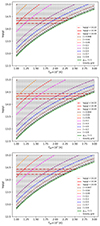 |
Fig. 1. Temperature – gravity grid for atmospheres composed purely of hydrogen (upper panel), purely of helium (middle panel), and of heavy elements (bottom panel). The gray dots show the gravity grid with Δg = 0.05 in logarithmic scale, because for Δg = 0.01, the figure would not be legible. The different dashed curves represent models with constant l at the values described in the legend. The horizontal solid red line displays the value of the gravity for the best-fit mass and radius measured by Nättilä et al. (2017), and the two horizontal dashed red lines correspond to the measured errors (see Sect. 2.3). |
Each individual point in Fig. 1 represents the model atmosphere computed using a grid of 1025 wavelength points in the range 0.01 − 25000 Å and a grid of 96 Thomson depths from 1e−7 to 7.5e+04. Both grids are equidistant in logarithmic scale.
The whole data set computed by us contains more than 45 000 models, which is the densest grid computed so far. For comparison, Suleimanov et al. (2011) presented a grid with 360 models. This grid was computed for only three values of the surface gravity (log(g) = 14.0, 14.3, and 14.6), for six chemical compositions, and for 20 values of the relative luminosities (starting from l = 0.001 up to l = 0.98). The grids computed by us follow the same range of relative luminosities.
The critical gravity given by Eq. (5) depends on the assumed effective temperature and on κes, the latter being a function of mass abundance of hydrogen, helium, and heavy elements given by X, Y, and Z, respectively (see Table 1 for the exact numbers). Thus, the value of the critical gravity is connected to the chemical abundance of the atmosphere. For atmospheres composed only of pure hydrogen (κes = 0.4), the value of the critical gravity is higher than the atmosphere composed only of helium (κes = 0.2) or an atmosphere with a solar composition (κes = 0.35) for the same effective temperature Teff. The relative luminosity for which the atmosphere reaches the critical gravity equals unity, and it is marked by green solid line in each panel of Fig. 1.
2.3. Neutron star models and ray-tracing
Models computed with ATM24 are local, meaning that they describe emission from the surface of the atmosphere. When radiation is to be transported correctly from the atmosphere to a distant observer and is to include all processes that occur in close proximity to the NS, the ray-tracing procedure must be used. Following our approach (Vincent et al. 2018), we used the open-source ray-tracing code GYOTO to transport spectra to the distant observer. We obtained the spacetime solution using the LORENE/NROTSTAR library, in particular, we estimated the value of the surface gravity for a chosen EoS model, corresponding to the particular values of the NS mass and radius. In the next step of our procedure, this surface gravity, together with effective temperature, was an input parameter in the code ATM24, and after the local spectrum was computed, it was ray-traced to the observer.
The selected benchmark EoS is a relativistic polytrope model, composed of identical relativistic particles of rest-mass m0, as defined4 in the LORENE library:
 (6)
(6)
where n is the numerical (baryon) density, p(n) is the pressure, e(n) is the mass-energy density, and μ0 = m0c2 is the chemical potential at zero pressure. The values of the parameters are the particle mass m0 = 1.66 × 10⁻³⁰ g, the polytropic index γ = 2.7, and the pressure coefficient κ = 0.013 in units of  , with ρnuc = 1.66 × 10²⁰ g m−3, nnuc = 0.1 fm−3.
With this choice, we produced a configuration consistent with the best-fit mass and radius obtained in Nättilä et al. (2017), as shown in Fig. 2 by the solid red line, intersecting the measured value marked by the central red dot, and the gray error bars in M and R correspond to the measurement errors. For comparison, we also show M(R) sequences obtained using realistic dense-matter EoSs solutions: the SLY4 EoS (Chabanat et al. 1998; Douchin & Haensel 2001), the BSK20 EoS developed by the Brussels-Montreal group (Potekhin et al. 2013), and the GM1Z0 EoS based on a relativistic mean field model (Weissenborn et al. 2012). These dense-matter EoSs were supplemented with the low-density part description of the NS crust of Haensel & Pichon (1994; for more detailed comparisons, see Bejger 2013).
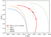 |
Fig. 2. NS mass-radius relations for selected EoSs. The dash-dotted blue curve presentes the SLY4 EOS, the dashed yellow curve shows the BSK20 EoS, and the dotted green curve shows GM1Z0 EoS. The red curve denotes the relativistic polytropic EoS consistent with the measurements of Nättilä et al. (2017), with dots marking the center of the error box and its boundaries. |
Subsequently, we ray-traced spectra for three values of the surface gravity that corresponded to the mass-radius values presented by red dots in Fig. 2, where central dot is a measurement, and the two edge dots are errors. The values of these surface gravities are marked by horizontal solid red lines (measured value), and dashed red lines (errors) in each panel of Fig. 1, meaning that ray-traced spectra span the whole effective temperature range for each chemical composition. In the case of the nonrotating spherical NS considered in this paper, the ray-traced spectra differ from the local spectra by only a factor 1 + z, where z is the gravitational redshift. Therefore, we prepared our grid of models composed of local spectra in the format required by the XSPEC fitting package. Nevertheless, a pipeline for computations of rotating NS atmospheres is ready and will be prepared in the near future.
3. Results
3.1. Temperature structure of the model atmospheres
The first direct result of our computations is an angle-dependent intensity spectrum from the stratified NS atmosphere, ray-traced in the gravitational field. The obtained spectral energy distribution may be directly fit to the observations, indicating the temperature and gravity on the NS surface. Nevertheless, in stellar atmospheres dominated by electron scattering, photons are created in the so-called thermalization layer (by thermal processes below the photosphere). In the thermalization layer, the local temperature T is higher than the effective temperature Teff, from which we conclude that the maximum of the Planck function of Bν(T) appears at a higher energy than the maximum of the Planck function of Bν(Teff). This effect has far-reaching consequences because the blackbody temperature obtained from fitting the continuum spectra is usually higher than the effective temperature Teff, and it is indicated as the color temperature Tc.
3.2. Color-correction factor
The color-correction factor is defined as the ratio of the frequency at which the best-fit spectrum displays the maximum to the peak of the blackbody spectrum at the effective temperature of an atmosphere. It can be directly described by the ratio of the color temperature to the effective temperature of the star as fc = Tc/Teff. The color-correction factor can increase to very high values in atmospheres that only take Thomson scattering into account because the true absorption in these atmospheres decreases to zero (see Madej 1974). In atmospheres that include Compton scattering, this factor is larger than unity, but lower than in the case of elastic electron scattering. For a fast estimation of the value of the color temperature either from a model or from an observed spectrum, we used the following formula:
 (7)
(7)
where kB is the Boltzmann constant, and Emax is the energy for which the spectrum of the NS at a given temperature Teff reaches maximum.
Another way to obtain the color temperature is the procedure of fitting the blackbody spectrum to our simulated or observed data by the minimalization of the sum
 (8)
(8)
where Fν is the simulated or the observed flux, and υ is the normalization factor. Our procedure started with finding the maximum emission and corresponding frequency, and then we took a range of frequencies around the maximum to make our fit appropriate. After we created a table of frequencies, we set the grid of temperatures starting from Teff of our model up to three times that temperature and divided it into M numbers of small intervals. We do not expect the color-correction factor to be higher than 3. Then we computed the renormalization factor in the following way:
 (9)
(9)
where vmax and vmin correspond to the frequencies around the maximum emission of the spectral curve. We used a χ2 test to determine the temperature of the blackbody spectrum that fits our simulated data best, which we attributed to the value of Tc. The frequencies around maximum were always adapted to each model atmosphere, and they might depend on different chemical composition. For instance, for a pure hydrogen atmosphere at a temperature of 1.5 × 10⁷ K, the energy range was from 8.1 × 10¹⁷ Hz up to 2.1 × 10¹⁸ Hz.
This fitting method allowed us to derive the color temperature in local spectra. In the case of a nonrotating NS, the hardening factor from ray-traced spectra was divided by 1 + z with respect to the same hardening factor for local models. In the first step, fc, 1 is the above factor computed from the ratio of the color temperature obtained simply from Eq. (7) and the effective temperature of the model Teff. In the second step, fc, 2 is the ratio of the color temperature, obtained from the blackbody fitting procedure to the local spectrum to the Teff of the model.
In Table 2 we show an example of the values of the color-correction factor for an effective temperature Teff = 1 × 10⁷ K and surface gravity log(g) = 14.34, the latter being the result of the best-fit mass and radius obtained by Nättilä et al. (2017).
Values of the color-correction factor for an effective temperature Teff = 1 × 10⁷ K and for log g = 14.34, which corresponds to an NS mass of 1.9 M⊙ and to a radius of 12.4 km.
In our models, the temperature structure is determined by two sources of monochromatic opacities. In deeper layers of the atmosphere, newly generated photons undergo free-free and bound-free absorption by ions, which heats the surrounding atmosphere. As the height increases (or the opacity decreases), the absorption cross section falls. Free-free absorption dominates until the effective Thompson depth is reached (τeff). Now, there are very few ions to provide enough capture cross section for absorption, so that scattering starts to dominate. At Teff ≥ 107 K, Compton scattering becomes important (Madej 1991a; Madej et al. 2004; Suleimanov et al. 2016). Cold electrons in the upper atmosphere efficiently exchange energy with high-energy photons, leading to an increase in temperature. An isothermal layer develops in the photosphere with T ≥ Teff, as presented in Figs. 3 and 4.
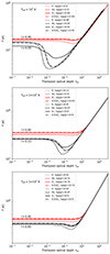 |
Fig. 3. Temperature structure for models with a fixed effective temperature Teff = 1, 2, and 3 × 10⁷ K (upper, middle, and bottom panel, respectively). Different chemical compositions are presented by different line styles given in the legend. Two relative luminosities are presented by red lines for l = 0.95 in each figure panel and by black lines for l = 0.05, l = 0.13, l = 0.65 in the upper, middle, and bottom panel, respectively. |
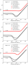 |
Fig. 4. Temperature structure for models with a fixed surface gravity equal to the measured value log(g) = 14.34, which corresponds to an NS mass 1.9 M⊙ and a radius of 12.4 km (middle panel; Nättilä et al. 2017), and the errors are log(g) = 13.70 (upper panel), and log(g) = 14.90 (bottom panel). The different chemical compositions are presented by different line styles given in the legend. Two relative luminosities are presented by red lines for l = 0.95 in the upper and middle panels, for l = 0.3 in the bottom panel, and by the black lines for l = 0.05, l = 0.13, l = 0.65 in the upper, middle, and bottom panel, respectively. |
Both effects combined cause a minimum in the temperature profile below the photosphere and a significant temperature rise in the uppermost layers of the atmosphere. The depth and location of the minimum depends on the value of the surface gravity and on the chemical composition (Fig. 3). For a luminous atmosphere, the temperature minimum is less pronounced and is also shifted toward higher optical depths. The local spectrum, presented by dashed lines in all panels of Fig. 5, deviates from the blackbody curve Bv(Teff) presented by dotted lines in the figure. All these features agree with previous papers on NS atmospheres (Madej 1991a; Madej et al. 2004; Suleimanov et al. 2016).
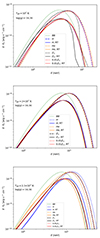 |
Fig. 5. Emergent spectra of the model atmospheres before (dashed lines) and after ray-tracing (solid lines), and emergent spectra of local blackbody emission (dotted line). The models were computed for a fixed effective temperature Teff = 1, 2, and 2.3 × 10⁷ K (upper, middle, and bottom panel, respectively) for all chemical compositions given by colors, and for a fixed value of surface gravity log(g) = 14.34, which corresponds to an NS mass of 1.9 M⊙ and a radius of 12.4 km. |
In Fig.4, the effect of the variation in Teff on the atmosphere structure is shown at constant log(g). The temperature structure depends on the chemical composition of the NS atmosphere. This is more evident at lower Teff. When we compare pure hydrogen NS atmospheres, their structures do not differ much from those of 0.01 Z⊙ with the same other input parameters. For He-rich atmospheres, the characteristic temperature jump occurs at lower optical depth than in case of other chemical abundances. Since models of solar abundance are composed of a mixture of many elements, their net effect is an erratic variation. At sufficiently high Teff, all elements are ionized and show similar variation.
3.3. Ray-traced spectra
The continuum spectra for the value of the surface gravity log(g) = 14.34 and for all chemical compositions are presented in Fig. 5 for three effective temperatures starting from Teff = 1 × 10⁷ K. The highest possible temperature for which the above gravity does not exceed the critical gravity for all considered abundances is Teff = 2.3 × 10⁷ K. In all figures, the spectra generated from the local ATM24 are represented by dashed lines and the ray-traced models by solid lines. The deviation from blackbody spectra (dotted green curve) is immediately apparent. This was extensively discussed previously and is summarized with the use of the color-correction factor in the section below.
In this section, we verify the correctness of our models according to the ray-tracing procedure used. Compared to the ATM24 model, all the ray-traced (RT) model spectra terminate at lower energies. This is a direct consequence of the gravitational redshift (z). The local intensity is reduced by a factor of 1+z (Vincent et al. 2018) as it reaches the observer. This has led to lower color-correction factor values.
We used a crude estimation of the redshift value from the spectrum and tried to back-calculate the mass-radius ratio as considered by the polytropic EoS in Sect. 2.3. We considered the shift in the energy that corresponds to the peak flux for both spectra computed by us, as shown in Fig. 6. Using the standard relation between an energy in which the local spectrum peaks at E′, and an energy for which the observed spectrum peaks at E, that is, E′/E = 1 + z, the z value is 0.37. Finally, for this redshift value, by using Eq. (2), we obtained an NS mass-radius ratio of 0.157. This roughly matches the mass of 1.9 M⊙ and radius of 12.4 km of NS used in this work and presented in Fig. 2. The above exercise proves that our numerical models fully take gravitational correction factors due to the compact nature of the NS into account.
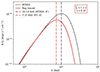 |
Fig. 6. Quantitative shift in peak energy due to redshift (z) from the local ATM24 model spectrum to ray-traced (RT) spectrum for Teff = 2 × 10⁷ K and log(g) = 14.34. The red box shows the redshift calculation from the standard relation between the energy of the local intensity peak E′, marked by the vertical dash-dotted black line, and energy of the observed intensity peak E, marked by the vertical red line of the same style. |
The overall spectral shape for the same effective temperature and surface gravity depends on the chemical abundance. It is interesting to note that H and He form two extremes in any type of variation in the temperature structure (Fig. 3) and continuum spectrum (Fig. 5). For the lowest effective temperature, only the He-like atmosphere spectrum stands out from the rest, especially for the high-energy end. The difference becomes larger with the rise in temperature, and it is clearly visible in the bottom panel of Fig. 5. The ray-tracing procedure does not change this trend.
In the case of a low effective temperature, Fig. 5, the Z⊙ curve for both model spectra and RT spectra is broken at higher photon energies. These are iron absorption edges at around 8–9 kev (Suleimanov et al. 2011). Similar features were reported by Nättilä et al. (2015), which are a result of the incomplete ionization of Fe ions and other heavy elements. The spectral curve is sensitive to metal abundances at higher effective temperatures, as shown in the bottom panel of Fig. 5.
3.4. Color-correction factor versus luminosity ratio
We used the convention to plot the color-correction factor versus luminosity ratio in Figs. 7 and 8, which we did not use before. Since the temperature and surface gravity both count for the luminosity ratio value, the first plot was made for one single effective temperature, and the second plot was given for a fixed value of the surface gravity, log g = 14.43. We calculated the factors for all local spectra, fc, 2, with the fitting procedure described in Sect. 3.2.
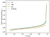 |
Fig. 7. Color-correction factor fc, 2, obtained with the fitting procedure described in Sect. 3.2, vs. luminosity for the models with a fixed value of the effective temperature Teff = 2 × 10⁷ K for all chemical compositions. |
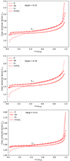 |
Fig. 8. Color-correction factors for local models fc, 2, obtained with the fitting procedure described in Sect. 3.2. The plots show the luminosity dependence for a fixed value of the surface gravity log(g) = 14.22 (top panel), log(g) = 14.34 (middle panel), and log(g) = 14.43 (bottom panel), i.e., the values inferred from the NS model (see Fig. 2), and for all chemical compositions. |
The color-correction factors from local spectra fc, 2 are presented for one case of a moderate value of the temperature Teff = 2 × 10⁷ K in Fig. 7, spanning all possible surface gravities and for all considered abundances. Fig. 8 shows color-correction factors as red lines for a reference measured value of the surface gravity log(g) = 14.34 (middle panel) and for the errors (top and bottom panels). In each case, all chemical compositions are presented. The obtained values of fc, 2 are consistent with previous estimates made by our group (Majczyna et al. 2005). The dependence on metallicity is clearly visible here. Pure hydrogen atmospheres present the largest color shift for a wide range of luminosities, except for the case when l ≥ 0.9, where metal-rich atmospheres display a higher color correction factor. Pure helium atmospheres always have color factors lower by 0.1 than pure hydrogen models, which is consistent with Suleimanov et al. (2011). This difference is due to the variation in the number density of free electrons, which are needed for the Compton process to be important. The main difference of our models to previously published work (Suleimanov et al. 2011) is the low-luminosity end of the dependence of the color-correction factor versus luminosity ratio. In the case of our models and for all considered abundances, the value of fc, 2 saturates at about 1.4 when the luminosity decreases. This discrepancy probably results from the differences between the Fortran procedures that compute Gaunt factors for the free-free absorption that are used by our groups.
Since our color-correction factor estimates are well derived for the wide range of l values, they may be applicable to a wide variety of systems such as the quiescent state of NS and X-ray bursters (l ≥ 0.8).
4. Conclusions
We presented a new grid of nonrotating NS models for hot stratified atmospheres resulting from radiative transfer computations. We focused on estimating the hardening factor for spectra of NS with a wide range of abundances and luminosities. The computational code ATM24 takes into account free-free and bound-free energy-dependent opacities of hydrogen, helium, and ions of heavy elements, including iron. By fitting a blackbody shape to local and ray-traced spectra near the highest emission region, the color-correction factors were calculated. They can be used to determine the spectral shape and NS parameters from observations.
The RT procedure accounts for the gravitational redshift suffered by photons emitted from an atmosphere. Photons leaving the photosphere of an NS are subjected to an immense gravitational potential that redshifts their energy for the distant observer. Additional effects can also take place, such as Doppler boosting and anisotropic emission. These effects need to be accounted for when analyzing the observed spectrum and estimating other quantities, such as the NS mass and radius (for example see: Vincent et al. 2018). The most prominent effect that contributes to a substantial difference in the color-correction factor is the gravitational redshift. Since the redshift factor z depends on the mass of the compact object, our calculations of the RT models and their use for a data analysis can place more reliable constraints on the NS mass and radius determination with a continuum-fitting method (Majczyna et al. 2005).
The composition of an NS atmosphere is a long-standing research question and is connected with the formation and evolution of an NS. We considered important elements that might comprise the NS atmosphere and showed how it affects the spectrum and temperature structure. The effect of gravity is to vary the density of lighter and heavier elements in the NS atmosphere. Depending on the physical processes involved after the formation of the NS, the atmosphere maybe dominated by H or He or by heavier elements such as Fe. Generally, accreting NSs leave behind a hydrogen-rich environment, while nonaccreting NSs are rich in iron (Ho et al. 2014). Nuclear burning processes leave behind helium or carbon (Ho et al. 2014). As shown by Zavlin et al. (1996), an iron atmosphere has a higher opacity than H or He atmospheres at a given photon energy. They also showed that at a given depth, an iron atmosphere has a higher temperature than an atmosphere that is composed of H or He.
We demonstrated that for a lower l value, the temperature minimum in the structure of an atmosphere for solar abundance (Z⊙ = 1) is almost never as low as in case of a low metallicity or pure hydrogen or helium atmospheres. The rise in temperature due to Compton scattering is also not sharp, unlike the other abundance curves. Due to the mixture of different opacities of lighter and heavier elements in Z⊙, the net effect is a washed-out temperature minimum.
We are not able to predict the redshift value for observed spectra of a NS since it depends on the assumed EoS. Therefore, only the direct fitting of the ray-traced spectra may give us realistic values of the mass and radius.
In a forthcoming project, we additionally plan to investigate the effect of rotation on the value of the color-correction factor. After this step is made, we can fully use our models to work with observations of hot NS emission, determine the main parameters such as the NS mass and radius, and finally, place constraints on the EoS of the dense matter under strong gravitational conditions.
The relativistic polytrope EoS is described in details under this link: https://lorene.obspm.fr/Refguide/classLorene_1_1Eos__bf__poly.html
Acknowledgments
This research was partially supported by the Polish National Science Center grants No. 2021/41/B/ST9/04110 and 2021/43/B/ST9/01714.
References
- Arnaud, K. A. 1996, in Astronomical Data Analysis Software and Systems V, eds. G. H. Jacoby, & J. Barnes, ASP Conf. Ser., 101, 17 [NASA ADS] [Google Scholar]
- Asplund, M., Grevesse, N., Sauval, A. J., & Scott, P. 2009, ARA&A, 47, 481 [NASA ADS] [CrossRef] [Google Scholar]
- Bejger, M. 2013, A&A, 552, A59 [NASA ADS] [CrossRef] [EDP Sciences] [Google Scholar]
- Beloborodov, A. M. 2002, ApJ, 566, L85 [Google Scholar]
- Chabanat, E., Bonche, P., Haensel, P., Meyer, J., & Schaeffer, R. 1998, Nucl. Phys. A, 635, 231 [NASA ADS] [CrossRef] [Google Scholar]
- Douchin, F., & Haensel, P. 2001, A&A, 380, 151 [NASA ADS] [CrossRef] [EDP Sciences] [Google Scholar]
- Ebisuzaki, T., Hanawa, T., & Sugimoto, D. 1984, PASJ, 36, 551 [Google Scholar]
- Foster, A. J., Ross, R. R., & Fabian, A. C. 1986, MNRAS, 221, 409 [NASA ADS] [CrossRef] [Google Scholar]
- Fujimoto, M. Y., & Taam, R. E. 1986, ApJ, 305, 246 [NASA ADS] [CrossRef] [Google Scholar]
- Gourgoulhon, E., Grandclément, P., Marck, J. A., Novak, J., & Taniguchi, K. 2016, LORENE: Spectral methods differential equations solver, Astrophysics Source Code Library [record ascl:1608.018] [Google Scholar]
- Guilbert, P. W. 1981, MNRAS, 197, 451 [NASA ADS] [Google Scholar]
- Guillot, S., Rutledge, R. E., & Brown, E. F. 2011, ApJ, 732, 88 [NASA ADS] [CrossRef] [Google Scholar]
- Haensel, P., & Pichon, B. 1994, A&A, 283, 313 [NASA ADS] [Google Scholar]
- Haensel, P., Potekhin, A. Y., & Yakovlev, D. G. 2007, Neutron Stars 1: Equation of State and Structure (New York: Springer), 326 [Google Scholar]
- Heinke, C. O., Rybicki, G. B., Narayan, R., & Grindlay, J. E. 2006, ApJ, 644, 1090 [NASA ADS] [CrossRef] [Google Scholar]
- Ho, W. C. G. 2014, in Magnetic Fields throughout Stellar Evolution, eds. P. Petit, M. Jardine, & H. C. Spruit, 302, 435 [NASA ADS] [Google Scholar]
- Ho, W. C. G., & Heinke, C. O. 2009, Nature, 462, 71 [NASA ADS] [CrossRef] [Google Scholar]
- Ho, W. C. G., Potekhin, A. Y., & Chabrier, G. 2008, ApJS, 178, 102 [NASA ADS] [CrossRef] [Google Scholar]
- Joss, P. C., & Madej, J. 2001, in Two Years of Science with Chandra, ed. A. Siemiginowska, 214 [Google Scholar]
- Joss, P. C., Stage, M. D., Madej, J., & Rozanska, A. 2004, in 35th COSPAR Scientific Assembly, 35, 3619 [NASA ADS] [Google Scholar]
- Lapidus, I. I., Syunyaev, R. A., & Titarchuk, L. G. 1986, Soviet Astron. Lett., 12, 383 [Google Scholar]
- London, R. A., Howard, W. M., & Taam, R. E. 1984, ApJ, 287, L27 [NASA ADS] [CrossRef] [Google Scholar]
- London, R. A., Taam, R. E., & Howard, W. M. 1986, ApJ, 306, 170 [Google Scholar]
- Madej, J. 1974, Acta Astron., 24, 327 [NASA ADS] [Google Scholar]
- Madej, J. 1989, ApJ, 339, 386 [NASA ADS] [CrossRef] [Google Scholar]
- Madej, J. 1991a, ApJ, 376, 161 [NASA ADS] [CrossRef] [Google Scholar]
- Madej, J. 1991b, Acta Astron., 41, 73 [NASA ADS] [Google Scholar]
- Madej, J. 1997, A&A, 320, 177 [NASA ADS] [Google Scholar]
- Madej, J., Joss, P. C., & Różańska, A. 2004, ApJ, 602, 904 [NASA ADS] [CrossRef] [Google Scholar]
- Madej, J., Różańska, A., Majczyna, A., & Należyty, M. 2017, MNRAS, 469, 2032 [NASA ADS] [CrossRef] [Google Scholar]
- Majczyna, A., & Madej, J. 2005, Acta Astron., 55, 349 [NASA ADS] [Google Scholar]
- Majczyna, A., Madej, J., Joss, P. C., & Różańska, A. 2005, A&A, 430, 643 [NASA ADS] [CrossRef] [EDP Sciences] [Google Scholar]
- Medin, Z., von Steinkirch, M., Calder, A. C., et al. 2016, ApJ, 832, 102 [NASA ADS] [CrossRef] [Google Scholar]
- Mori, K., & Ho, W. C. G. 2007, MNRAS, 377, 905 [NASA ADS] [CrossRef] [Google Scholar]
- Nagirner, D. I., & Poutanen, J. 1993, A&A, 275, 325 [NASA ADS] [Google Scholar]
- Nättilä, J., Suleimanov, V. F., Kajava, J. J. E., & Poutanen, J. 2015, A&A, 581, A83 [NASA ADS] [EDP Sciences] [Google Scholar]
- Nättilä, J., Miller, M. C., Steiner, A. W., et al. 2017, A&A, 608, A31 [NASA ADS] [CrossRef] [EDP Sciences] [Google Scholar]
- Özel, F., & Freire, P. 2016, ARA&A, 54, 401 [Google Scholar]
- Pomraning, G. C. 1973, The Equations of Radiation Hydrodynamics (Oxford: Pergamon Press) [Google Scholar]
- Potekhin, A. Y., Fantina, A. F., Chamel, N., Pearson, J. M., & Goriely, S. 2013, A&A, 560, A48 [NASA ADS] [CrossRef] [EDP Sciences] [Google Scholar]
- Poutanen, J. 2020, A&A, 640, A24 [NASA ADS] [CrossRef] [EDP Sciences] [Google Scholar]
- Rauch, T., Suleimanov, V., & Werner, K. 2008, A&A, 490, 1127 [NASA ADS] [CrossRef] [EDP Sciences] [Google Scholar]
- Stage, M., Joss, P., & Madej, J. 2002a, in 34th COSPAR Scientific Assembly, 34, 2593 [NASA ADS] [Google Scholar]
- Stage, M. D., Joss, P. C., & Madej, J. 2002b, in Neutron Stars in Supernova Remnants, eds. P. O. Slane, & B. M. Gaensler, ASP Conf. Ser., 271, 327 [NASA ADS] [Google Scholar]
- Stage, M. D., Joss, P. C., Madej, J., & Różańska, A. 2004, Adv. Space Res., 33, 605 [NASA ADS] [CrossRef] [Google Scholar]
- Suleimanov, V., Poutanen, J., & Werner, K. 2011, A&A, 527, A139 [NASA ADS] [CrossRef] [EDP Sciences] [Google Scholar]
- Suleimanov, V., Poutanen, J., & Werner, K. 2012, A&A, 545, A120 [NASA ADS] [CrossRef] [EDP Sciences] [Google Scholar]
- Suleimanov, V. F., Klochkov, D., Pavlov, G. G., & Werner, K. 2014, ApJS, 210, 13 [Google Scholar]
- Suleimanov, V. F., Poutanen, J., Klochkov, D., & Werner, K. 2016, Eur. Phys. J. A, 52, 20 [NASA ADS] [CrossRef] [Google Scholar]
- van Paradijs, J. 1979, ApJ, 234, 609 [NASA ADS] [CrossRef] [Google Scholar]
- van Paradijs, J., & Lewin, W. H. G. 1987, A&A, 172, L20 [NASA ADS] [Google Scholar]
- Vincent, F. H., Paumard, T., Gourgoulhon, E., & Perrin, G. 2011, CQG, 28, 225011 [NASA ADS] [CrossRef] [Google Scholar]
- Vincent, F. H., Gourgoulhon, E., & Novak, J. 2012, CQG, 29, 245005 [Google Scholar]
- Vincent, F. H., Bejger, M., Różańska, A., et al. 2018, ApJ, 855, 116 [NASA ADS] [CrossRef] [Google Scholar]
- Webb, N. A., & Barret, D. 2007, ApJ, 671, 727 [Google Scholar]
- Weissenborn, S., Chatterjee, D., & Schaffner-Bielich, J. 2012, Phys. Rev. C, 85, 065802 [CrossRef] [Google Scholar]
- Zavlin, V. E., Pavlov, G. G., & Shibanov, Y. A. 1996, A&A, 315, 141 [NASA ADS] [Google Scholar]
All Tables
Values of the color-correction factor for an effective temperature Teff = 1 × 10⁷ K and for log g = 14.34, which corresponds to an NS mass of 1.9 M⊙ and to a radius of 12.4 km.
All Figures
|
Fig. 1. Temperature – gravity grid for atmospheres composed purely of hydrogen (upper panel), purely of helium (middle panel), and of heavy elements (bottom panel). The gray dots show the gravity grid with Δg = 0.05 in logarithmic scale, because for Δg = 0.01, the figure would not be legible. The different dashed curves represent models with constant l at the values described in the legend. The horizontal solid red line displays the value of the gravity for the best-fit mass and radius measured by Nättilä et al. (2017), and the two horizontal dashed red lines correspond to the measured errors (see Sect. 2.3). |
| In the text | |
|
Fig. 2. NS mass-radius relations for selected EoSs. The dash-dotted blue curve presentes the SLY4 EOS, the dashed yellow curve shows the BSK20 EoS, and the dotted green curve shows GM1Z0 EoS. The red curve denotes the relativistic polytropic EoS consistent with the measurements of Nättilä et al. (2017), with dots marking the center of the error box and its boundaries. |
| In the text | |
|
Fig. 3. Temperature structure for models with a fixed effective temperature Teff = 1, 2, and 3 × 10⁷ K (upper, middle, and bottom panel, respectively). Different chemical compositions are presented by different line styles given in the legend. Two relative luminosities are presented by red lines for l = 0.95 in each figure panel and by black lines for l = 0.05, l = 0.13, l = 0.65 in the upper, middle, and bottom panel, respectively. |
| In the text | |
|
Fig. 4. Temperature structure for models with a fixed surface gravity equal to the measured value log(g) = 14.34, which corresponds to an NS mass 1.9 M⊙ and a radius of 12.4 km (middle panel; Nättilä et al. 2017), and the errors are log(g) = 13.70 (upper panel), and log(g) = 14.90 (bottom panel). The different chemical compositions are presented by different line styles given in the legend. Two relative luminosities are presented by red lines for l = 0.95 in the upper and middle panels, for l = 0.3 in the bottom panel, and by the black lines for l = 0.05, l = 0.13, l = 0.65 in the upper, middle, and bottom panel, respectively. |
| In the text | |
|
Fig. 5. Emergent spectra of the model atmospheres before (dashed lines) and after ray-tracing (solid lines), and emergent spectra of local blackbody emission (dotted line). The models were computed for a fixed effective temperature Teff = 1, 2, and 2.3 × 10⁷ K (upper, middle, and bottom panel, respectively) for all chemical compositions given by colors, and for a fixed value of surface gravity log(g) = 14.34, which corresponds to an NS mass of 1.9 M⊙ and a radius of 12.4 km. |
| In the text | |
|
Fig. 6. Quantitative shift in peak energy due to redshift (z) from the local ATM24 model spectrum to ray-traced (RT) spectrum for Teff = 2 × 10⁷ K and log(g) = 14.34. The red box shows the redshift calculation from the standard relation between the energy of the local intensity peak E′, marked by the vertical dash-dotted black line, and energy of the observed intensity peak E, marked by the vertical red line of the same style. |
| In the text | |
|
Fig. 7. Color-correction factor fc, 2, obtained with the fitting procedure described in Sect. 3.2, vs. luminosity for the models with a fixed value of the effective temperature Teff = 2 × 10⁷ K for all chemical compositions. |
| In the text | |
|
Fig. 8. Color-correction factors for local models fc, 2, obtained with the fitting procedure described in Sect. 3.2. The plots show the luminosity dependence for a fixed value of the surface gravity log(g) = 14.22 (top panel), log(g) = 14.34 (middle panel), and log(g) = 14.43 (bottom panel), i.e., the values inferred from the NS model (see Fig. 2), and for all chemical compositions. |
| In the text | |
Current usage metrics show cumulative count of Article Views (full-text article views including HTML views, PDF and ePub downloads, according to the available data) and Abstracts Views on Vision4Press platform.
Data correspond to usage on the plateform after 2015. The current usage metrics is available 48-96 hours after online publication and is updated daily on week days.
Initial download of the metrics may take a while.