| Issue |
A&A
Volume 687, July 2024
|
|
|---|---|---|
| Article Number | L9 | |
| Number of page(s) | 6 | |
| Section | Letters to the Editor | |
| DOI | https://doi.org/10.1051/0004-6361/202450374 | |
| Published online | 05 July 2024 | |
Letter to the Editor
The “C”: The large Chameleon-Musca-Coalsack cloud
1
Max Planck Institute for Astrophysics, Karl-Schwarzschild-Straße 1, 85748 Garching bei München, Germany
e-mail: This email address is being protected from spambots. You need JavaScript enabled to view it.
2
Ludwig Maximilian University of Munich, Geschwister-Scholl-Platz 1, 80539 München, Germany
3
Institute for Astronomy, University of Vienna, Türkenschanzstrasse 17, 1180 Vienna, Austria
4
Center for Astrophysics | Harvard & Smithsonian, 60 Garden St., Cambridge, MA 02138, USA
5
Excellence Cluster ORIGINS, Boltzmannstraße 2, 85748 Garching bei München, Germany
Received:
15
April
2024
Accepted:
7
June
2024
Abstract
Recent advancements in 3D dust mapping have transformed our understanding of the Milky Way’s local interstellar medium, enabling us to explore its structure in three spatial dimensions for the first time. In this Letter, we use the most recent 3D dust map by Edenhofer et al. to study the well-known Chameleon, Musca, and Coalsack cloud complexes, located about 200 pc from the Sun. We find that these three complexes are not isolated but rather connect to form a surprisingly well-defined half-ring, constituting a single C-shaped cloud with a radius of about 50 pc, a thickness of about 45 pc, and a total mass of about 5 × 10⁴ M⊙, or 9 × 10⁴ M⊙ if including everything in the vicinity of the C-shaped cloud. Despite the absence of an evident feedback source at its center, the dynamics of young stellar clusters associated with the C structure suggest that a single supernova explosion about 4 Myr–10 Myr ago likely shaped this structure. Our findings support a single origin story for these cloud complexes, suggesting that they were formed by feedback-driven gas compression, and offer new insights into the processes that govern the birth of star-forming clouds in feedback-dominated regions, such as the Scorpius-Centaurus association.
Key words: ISM: clouds / dust / extinction / ISM: structure / ISM: individual objects: Musca / ISM: individual objects: Coalsack / ISM: individual objects: Chameleon
© The Authors 2024
 Open Access article, published by EDP Sciences, under the terms of the Creative Commons Attribution License (https://creativecommons.org/licenses/by/4.0), which permits unrestricted use, distribution, and reproduction in any medium, provided the original work is properly cited.
This article is published in open access under the Subscribe to Open model.
Open access funding provided by Max Planck Society.
1. Introduction
For over a hundred years, our understanding of the interstellar medium (ISM) has been limited to 2D projections. Analysis of 2D projections, while a mainstay in traditional studies of the ISM, can create a deceptive picture of the true and complex 3D structures of the ISM. For example, atomic and molecular clouds can appear as distinct or overlapping entities, which obscures their true spatial relationships. This illusion is especially problematic when clouds exhibit similar radial velocities, making it nearly impossible to distinguish their boundaries and depths using traditional observational methods.
The0]Please provide the missing City name for the Affiliation 4. nearby molecular clouds of Chameleon, Musca, and Coalsack – long suspected of being physically associated with one another – are a potential example of this type of confusion (Corradi et al. 1997, 2004). However, their seemingly distinct appearances in the 2D plane of the sky has complicated any firm conclusions regarding a possible physical association. This projected view is potentially hiding diffuse connections that could shed new light on their origin and evolution.
In recent years, the proliferation of 3D dust maps has begun a revolution in the field (e.g., Edenhofer et al. 2024b; Leike & Enßlin 2019; Vergely et al. 2022; Lallement et al. 2022, 2019, 2018; Capitanio et al. 2017; Babusiaux et al. 2020; Hottier et al. 2020; Green et al. 2019, 2018; Leike et al. 2022; Chen et al. 2019; Rezaei Kh. & Kainulainen 2022; Rezaei Kh. et al. 2020, 2018, 2017; Dharmawardena et al. 2022). These new maps capitalize on the astrometric data from the ESA Gaia satellite (Gaia Collaboration 2023) and have emerged as powerful tools for unraveling the complex volume density distribution of gas within the local Milky Way, providing unprecedented insights into the structure and dynamics of molecular clouds from kiloparsec down to parsec scales (Zucker et al. 2023, 2018, 2019, 2020, 2021; Alves et al. 2020; Konietzka et al. 2024; Kuhn et al. 2023; Posch et al. 2023).
Chameleon, Musca, and Coalsack are among the closest molecular clouds to Earth, at a distance of about 200 pc (see, e.g., Zucker et al. 2021; Corradi et al. 2004). Chameleon has been extensively studied for its active star formation (e.g., Luhman 2008; Belloche et al. 2011; Persi et al. 2003; Tsitali et al. 2015) and Musca for its simple filamentary structure and subsonic nature (e.g., Mizuno et al. 1998; Hacar et al. 2016; Kainulainen et al. 2016). Coalsack, despite being one of the few dark clouds visible to the naked eye, is one of the least studied nearby clouds, probably because it is not star-forming and is seen against the complicated background of the Galactic plane (e.g., Nyman 2008; Beuther et al. 2011). So far, all three clouds have been treated as separate entities, and conflicting origin stories have been proposed for each. For example, Musca, is hypothesized to have been shaped by magnetic fields, by the dissipation of supersonic turbulence, by a cloud–cloud collision, or a combination of these processes (Cox et al. 2016; Tritsis & Tassis 2018; Tritsis et al. 2022; Bonne et al. 2020a,b; Yahia et al. 2021; Kaminsky et al. 2023).
In this Letter we study the Chameleon, Musca, and Coalsack region from a new perspective, namely, in full spatial 3D. Using the 3D dust map from Edenhofer et al. (2024b), we characterize the topology and mass of this region and analyze the relationship between the three molecular clouds. In addition, we analyze the dynamics of young stellar clusters (YSO clusters) embedded in Chameleon and Coalsack as a proxy for the large-scale dynamics of the gas.
2. Methods and results
We used the 3D reconstruction of the interstellar dust distribution presented in Edenhofer et al. (2024b) throughout our analysis. The reconstruction is based on the catalog described in Zhang et al. (2023), which in turn is based on the ESA Gaia DR3 BP/RP spectra (Gaia Collaboration 2023). Using the stellar extinction and distances in the catalog, Edenhofer et al. (2024b) reconstructed the 3D distribution of interstellar dust. The map extends to 1.25 kpc from the Sun and achieves 14′ angular resolution and parsec-scale distance resolution. Edenhofer et al. (2024b) discretized the modeled 3D space into logarithmically spaced distance voxels and equal-area plane-of-sky voxels. In this discretized space, they represent the logarithm of the differential dust extinction using a Gaussian process model (Edenhofer et al. 2022). The inference uses the software package NIFTy (Edenhofer et al. 2024a).
Edenhofer et al. (2024b) have created one of the highest resolution 3D dust maps of the local Milky Way. Unlike other 3D dust maps in the literature, it focuses on a relatively small volume (cf. Green et al. 2019), but resolves the structures within this volume with high (parsec-scale) resolution, comparable to Leike et al. (2020). Compared to Leike et al. (2020), it reconstructs a much larger volume and yields a higher dynamic range thanks to the new Gaia data. The methodology extends that from Leike et al. (2020) and employs its non-parametrically inferred correlation kernel. Furthermore, the model strictly enforces physical constraints, such as positive definiteness of differential interstellar dust densities, and rigorously incorporates the uncertainties on the distances to stars. The inference algorithm used has been extensively proven in real-world applications (see Galan et al. 2024; Arras et al. 2022; Leike & Enßlin 2019; Leike et al. 2020; Mertsch & Phan 2023; Roth et al. 2023a; Hutschenreuter et al. 2023, 2022; Tsouros et al. 2024; Roth et al. 2023b) and is provably exact in the linear regime (Knollmüller & Enßlin 2019).
2.1. Topology
Using the 3D map of the distribution of interstellar dust from Edenhofer et al. (2024b), we analyzed the region around Chameleon, Musca, and Coalsack. For convenience, we interpolated the 3D map with irregularly spaced voxels to a regular Cartesian and a regular spherical grid using the scripts provided by the authors online1 and distributed as part of the Python package dustmaps (Green 2018). We find that all three molecular clouds are embedded in a large 3D structure that forms a C-shaped half-ring. The structure lies at the edge of the Local Bubble (Zucker et al. 2022; O’Neill et al. 2024; Pelgrims et al. 2020), close to the Scorpius-Centaurus association. Due to obscuration and projection effects, the peculiar C shape is only revealed using 3D reconstructions of interstellar dust. In an ordinary 2D plane-of-sky projection, the diffuse bridges connecting the molecular clouds become indistinguishable from faint dust extinction at larger distances.
Figure 1 shows the extinction within the region over the range 335° to 275° in Galactic longitude and −40° to 15° in Galactic latitude. The first panel shows the Planck 2013 extragalactic E(B − V) extinction of interstellar dust (Planck Collaboration XI 2014) converted to AV via AV = 3.1 ⋅ E(B − V). The C-shaped structure is almost completely obscured. The second panel shows the 3D interstellar dust map integrated over a distance of 55 pc (from 165 pc to 220 pc). Here, the C-shaped structure appears as a single coherent structure that hosts Chameleon, Musca, and Coalsack. The individual dense molecular clouds are connected through faint lanes of interstellar dust extinction. Thanks to the 3D distance selection, the figure shows this region free of confusion stemming from extinction at farther distances.
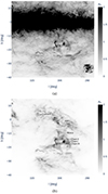 |
Fig. 1. Plane-of-sky region toward the C of the posterior mean of Edenhofer et al. (2024b). Panel a: Planck 2013 extragalactic E(B − V) extinction toward the C converted to AV via AV = 3.1 ⋅ E(B − V). Panel b: visual extinction, AV, between 165 pc and 220 pc toward the C-shaped structure in the 3D interstellar dust map. Spurs of Lupus are seen on the left edge. Both panels display the extinction in units of magnitude, and the colorbars are linear but clipped at an extinction of AV = 2 mag. |
With 3D interstellar dust maps, we are not restricted to plane-of-sky projections and can instead explore the distribution of interstellar dust in full spatial 3D. In Fig. 2 we show the isodensity surface in full spatial 3D with a total hydrogen nucleus density of approximately nH = 4.5 cm−3 (cf. Zucker et al. 2021; 0.98 quantile of the 3D dust density in the selected volume; see O’Neill et al. 2024 on how to convert the units of the 3D dust density to nH). The outline traces the C-shaped spine observed in Fig. 1. The isodensity surface fully envelops the half-ring that includes the Chameleons, Musca, and Coalsack molecular clouds. We term the C-shaped structure the “C.”
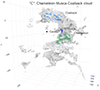 |
Fig. 2. 3D view of the isodensity surface of the posterior mean of the 3D dust map of Edenhofer et al. (2024b) within the Cartesian selection given in Table 1, showing the C. High-density structures (nH ≥ 23.3 cm−3; the 10 000 highest-density points of a 1 pc Cartesian interpolation of the C) toward Chameleon are color-coded in green (290° ≤l ≤ 306° and −21° ≤b ≤ −12°), toward Musca in violet (300° ≤l ≤ 302.5° and −13° ≤b ≤ −7.25°), and toward Coalsack in blue (300° ≤l ≤ 318° and 0.5° ≤b ≤ 7.5°). An interactive version of this figure is available at https://faun.rc.fas.harvard.edu/gedenhofer/perm/C/C_Chameleon_Musca_Coalsack_cloud.html. |
Based on its suggestive half-ring structure, we defined a center for the C. We defined it to lie below Coalsack in Galactic X and Y and slightly above the Galactic Z of the two Chameleons. Specifically, we set the center to be at Galactic X = 138 pc, Y = −140 pc, and Z = −33 pc (Galactic l = 314.6°, b = −9.5°, and d = 199.3 pc; see the interactive Fig. 2).
Relative to the center location, we defined a radius using the volume filling fraction of interstellar dust. We find that the volume filling fraction reaches a maximum at a distance of 48 pc, and we assume this to be the radius of the C. This estimate is robust with respect to different posterior samples of the dust distribution from Edenhofer et al. (2024b). The full width at half maximum (FWHM) of the peak is 47 ± 2 pc, and most of the dust lies within 80 pc of the center (the ceiling of the more distant edge of the FWHM).
We find that the C is almost perfectly parallel to the Galactic Z axis. Given its proximity to the Galactic disk, this makes it perpendicular to the line of sight. To quantify the inclination, we selected the 10 000 highest-density points of a 1 pc interpolation of the 3D dust map within 20 ≤ X ≤ 230 pc, −240 ≤ Y ≤ −90 pc, and −185 ≤ Z ≤ 50 pc and decomposed them with a singular value decomposition into a plane. We find that the Galactic Z axis and the plane’s normal vector form an 86° angle (two-thirds of the samples are within ±1°) and the inclination between the line of sight toward the center and the fitted plane to be 72° (two-thirds of the samples are within ±1°). Table 1 summarizes the key properties of the C.
Key properties of the C.
To estimate the mass, we again utilized the 3D interstellar dust density. We integrated the mass from the center out to a distance of 80 pc or the edge of the Cartesian selection given in Table 1, whichever is lower, and find the mass of everything within the vicinity of the C to be (9.34 ± 0.03) × 104 M⊙ (with the statistical uncertainty covering the 0.16 to 0.84 quantile of the interstellar 3D dust map). This mass estimate is roughly between the total mass of everything above a density of nH = 1 cm−3 and nH = 2 cm−3 within the Cartesian selection given in Table 1, (1.12 ± 0.01)×105 M⊙ and (8.00 ± 0.08)×104 M⊙, respectively. The mass of everything within the isosurface shown in Fig. 2 (i.e., above approximately nH = 4.5 cm−3) is (5.05 ± 0.03) × 104 M⊙. Details on how we computed the mass are provided in Appendix A.
2.2. Dynamics
To investigate the dynamics of the peculiar C-shaped structure, we studied YSO clusters embedded in the C. We used the Ratzenböck et al. (2023b) and Hunt & Reffert (2023) catalogs, applying the following cuts to the Hunt & Reffert (2023) catalog: logAge ≤ log10(30 Myr), astrometric S/N(SNR)≥5, and 50th percentile of color magnitude diagram (CMD) class ≥0.5 (cf. Hunt & Reffert 2023). Nested inside the C, we find three YSO clusters: Centaurus-Far (HSC 2630 in Hunt & Reffert 2023), Chameleon I (Hunt & Reffert 2023; Ratzenböck et al. 2023b), and Chameleon II (Ratzenböck et al. 2023b). In the following, we use the velocities given in Ratzenböck et al. (2023b).
The two Chameleons are embedded in the dense centers of the C, while Centaurus-Far lies at its edge. In contrast to the two Chameleon clusters, Centaurus-Far is strongly extended (see the updated online figure2 from Ratzenböck et al. 2023a) and encompasses both mostly dust-free regions and dense parts of Coalsack. Even though Centaurus-Far is not exclusively in the densest regions of the C, as a YSO cluster it likely still traces the overall gas motion of this region.
Relative to the local standard of rest (Schönrich et al. 2010), we find that the two Chameleon clusters are moving in the negative Galactic Z direction more strongly than Centaurus-Far. This implies that the C is expanding at least in the Galactic Z direction. We find no significant relative motion in the Galactic X and Y directions. If we assign our center point a hypothetical velocity of  with v▫ the velocities of Centaurus-Far and the two Chameleons, respectively, we find that Centaurus-Far moves up and the two Chameleons move down relative to the center. Their velocity relative to the center is 3 km s−1 for Centaurus-Far and 4 km s−1 and 2 km s−1 for the two Chameleons. In Galactic Z, the expansion is 1.9 km s−1 to 2.7 km s−1. We validate the relative velocities in Appendix B and find that the velocity uncertainty is on the order of the relative velocities, making this finding noteworthy but highly uncertain. We note that other tracers for the velocity, such as HI or CO, are unavailable since, in addition to obscuration and confusion, the inclination of the C results in its expansion being perpendicular to the line of sight.
As the YSOs clusters are embedded in the C, we propose that not only do the cluster move away from the center at an average velocity of 2 km s−1–3 km s−1, but the whole C expands at an average velocity of 2 km s−1–3 km s−1. Moving the mass in the vicinity of the C at this speed requires a significant amount of energy. Specifically, moving 9 × 10⁴ M⊙ at 2 km s−1–3 km s−1 requires an energy input of 4 × 1048 erg–8 × 1048 erg. This energy input is ≈1% of the total energy release of a supernova feedback event and on the order of the expected kinetic energy input of a supernova (Kim & Ostriker 2015).
2.3. Age
We analyzed the relative position of the clusters in the past by propagating their current position and velocity back in time using the software package galpy and the MWPotential2014 Galactic potential (Bovy 2015). In doing so, we neglected other gravitational forces such as the cluster’s own gravitational potential, gravitational forces due to nearby molecular clouds, and any other acceleration not due to the Milk Way’s potential. We find that the clusters have been approaching each other in the past 4 Myr–10 Myr. Relative to the moving center with the center velocity described above, Centaurus-Far got the closest, with a minimum separation of 25 pc from the center, while the two Chameleons got as close as 46 pc and 40 pc to the center in the last 10 Myr. The observation is robust with respect to the precise choice of center velocity, and the minimum separations vary by 10 pc or less if we assume the velocity of the center to be the average velocity of all YSO clusters in the vicinity (see Sect. 2.2). Given the large uncertainty in the velocities and ages and the simplistic model, these discrepancies appear modest, and the velocities and ages seem to be in good agreement with the hypothesis of an expanding half-ring.
Figure 3 shows the C in Cartesian X − Z projections. The three clusters and their trace-backs relative to the center are shown with colored lines.
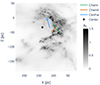 |
Fig. 3. Cartesian X − Z projections of the C. The colorbar is linear and clipped at AV = 1.5 mag. The traced-back clusters relative to the center are shown as colored lines. The solid lines show the traces of the cluster up to their 0.84-age quantile, while the dash lines show the traces back to −10 Myr whenever their 0.84-age quantile is lower. See the interactive version of Fig. 2 and toggle on the clusters to see them in full spatial 3D. |
2.4. Caveats
We have determined the shape and mass of the C with considerable accuracy using 3D interstellar dust maps. However, the dynamics and energy calculations remain uncertain. The C’s overall shape and the velocities of the YSO clusters suggest it may be an expanding half-ring, but our analysis is constrained by the limited number of YSO clusters observed. The uncertainties in the velocity measurements are comparable to the relative uncertainties, further complicating the analysis. In addition to the velocity uncertainties, the cause for the velocities is not known, and they might be purely turbulent in nature. Finally, although the C surrounds a largely empty space, there is evidence of spurs of interstellar dust at its center, as shown in Fig. 3.
In the future, we hope that better velocity measurements will help us quantify the motion of the C much more thoroughly. However, even much improved velocity uncertainties will not enable us to determine whether they are turbulent or driven by expansion. Considering the peculiar shape of the C, we believe turbulence alone is unlikely to be the sole cause.
3. Discussion and conclusion
Three-dimensional maps of interstellar dust have unlocked new ways to explore the intricate structures within the ISM in comprehensive 3D detail. Using these maps, we have established that the Chameleon, Musca, and Coalsack molecular clouds are spatially connected, forming a C-shaped structure that encompasses a striking, well-defined cavity. This structure, which we refer to as the C, is a half-ring structure with a radius of approximately 50 pc and a mass of about  , or 9 × 10⁴ M⊙ including everything in the vicinity of the C-shaped cloud. The C extends roughly 50° in both longitude and latitude, and has a depth of about 55 pc. The structure is discernible only through 3D reconstructions of interstellar dust, as obscuration and projection effects obscure it in conventional 2D views.
We propose a single origin for all three molecular clouds comprising the C. The orbits of clusters in the C are indicative of an expansion that, when combined with the mass of the C, requires the amount of energy released by a single supernova explosion. We suggest that a singular supernova explosion shaped an existing dense cloud into the C between 4 Myr and 10 Myr ago.
The realization that the Chameleon, Musca, and Coalsack molecular clouds are interconnected in 3D space introduces a novel perspective for their study. These previously distinct clouds are now understood to be parts of a single large cloud, the C. This broader context is especially significant for understanding Musca, for which a large body of observational work has been undertaken over the last decade to explain its formation. Viewing Musca within the scope of the C suggests a relatively simple formation mechanism: cloud formation on an expanding ring, likely driven by stellar feedback. This insight suggests that feedback-driven expansion is the primary cause for the shape of Musca (see Inutsuka et al. 2015; Ntormousi et al. 2017, for the role of magnetic fields) and calls for a new analysis of the existing data on this cloud. This new perspective on Musca’s formation and shape is a reminder that the environment in which a molecular cloud resides can significantly influence its formation mechanism and morphology. This work highlights the importance of considering the broader context offered by the new 3D dust maps when interpreting molecular cloud formation and evolution.
Acknowledgments
The authors would like to thank Cameren Swiggum for many helpful comments and discussions throughout the work. The authors would like to thank the anonymous referee for their very constructive and fruitful feedback. Gordian Edenhofer acknowledges that support for this work was provided by the German Academic Scholarship Foundation in the form of a PhD scholarship (“Promotionsstipendium der Studienstiftung des Deutschen Volkes”). This work was co-funded by the European Union (ERC, ISM-FLOW, 101055318). Views and opinions expressed are, however, those of the author(s) only and do not necessarily reflect those of the European Union or the European Research Council. Neither the European Union nor the granting authority can be held responsible for them.
References
- Abdurro’uf, Accetta, K., Aerts, C., et al. 2022, ApJS, 259, 35 [NASA ADS] [CrossRef] [Google Scholar]
- Alves, J., Zucker, C., Goodman, A. A., et al. 2020, Nature, 578, 237 [NASA ADS] [CrossRef] [Google Scholar]
- Arras, P., Frank, P., Haim, P., et al. 2022, Nat. Astron., 6, 259 [NASA ADS] [CrossRef] [Google Scholar]
- Babusiaux, C., Fourtune-Ravard, C., Hottier, C., Arenou, F., & Gómez, A. 2020, A&A, 641, A78 [NASA ADS] [CrossRef] [EDP Sciences] [Google Scholar]
- Belloche, A., Schuller, F., Parise, B., et al. 2011, A&A, 527, A145 [NASA ADS] [CrossRef] [EDP Sciences] [Google Scholar]
- Beuther, H., Kainulainen, J., Henning, T., Plume, R., & Heitsch, F. 2011, A&A, 533, A17 [NASA ADS] [CrossRef] [EDP Sciences] [Google Scholar]
- Bonne, L., Bontemps, S., Schneider, N., et al. 2020a, A&A, 644, A27 [EDP Sciences] [Google Scholar]
- Bonne, L., Schneider, N., Bontemps, S., et al. 2020b, A&A, 641, A17 [NASA ADS] [CrossRef] [EDP Sciences] [Google Scholar]
- Bovy, J. 2015, ApJS, 216, 29 [NASA ADS] [CrossRef] [Google Scholar]
- Buder, S., Sharma, S., Kos, J., et al. 2021, MNRAS, 506, 150 [NASA ADS] [CrossRef] [Google Scholar]
- Capitanio, L., Lallement, R., Vergely, J. L., Elyajouri, M., & Monreal-Ibero, A. 2017, A&A, 606, A65 [NASA ADS] [CrossRef] [EDP Sciences] [Google Scholar]
- Chen, B. Q., Huang, Y., Yuan, H. B., et al. 2019, MNRAS, 483, 4277 [Google Scholar]
- Corradi, W. J. B., Franco, G. A. P., & Knude, J. 1997, A&A, 326, 1215 [NASA ADS] [Google Scholar]
- Corradi, W. J. B., Franco, G. A. P., & Knude, J. 2004, MNRAS, 347, 1065 [NASA ADS] [CrossRef] [Google Scholar]
- Cox, N. L. J., Arzoumanian, D., André, P., et al. 2016, A&A, 590, A110 [NASA ADS] [CrossRef] [EDP Sciences] [Google Scholar]
- Dharmawardena, T. E., Bailer-Jones, C. A. L., Fouesneau, M., & Foreman-Mackey, D. 2022, A&A, 658, A166 [NASA ADS] [CrossRef] [EDP Sciences] [Google Scholar]
- Draine, B. T. 2003, ARA&A, 41, 241 [NASA ADS] [CrossRef] [Google Scholar]
- Draine, B. T. 2009, in Cosmic Dust - Near and Far, eds. T. Henning, E. Grün, & J. Steinacker, ASP Conf. Ser., 414, 453 [NASA ADS] [Google Scholar]
- Edenhofer, G., Leike, R. H., Frank, P., & Enßlin, T. A. 2022, arXiv e-prints [arXiv:2206.10634] [Google Scholar]
- Edenhofer, G., Frank, P., Roth, J., et al. 2024a, J. Open Source Software, 9, 6593 [NASA ADS] [CrossRef] [Google Scholar]
- Edenhofer, G., Zucker, C., Frank, P., et al. 2024b, A&A, 685, A82 [NASA ADS] [CrossRef] [EDP Sciences] [Google Scholar]
- Gaia Collaboration (Vallenari, A., et al.) 2023, A&A, 674, A1 [NASA ADS] [CrossRef] [EDP Sciences] [Google Scholar]
- Galan, A., Caminha, G. B., Knollmüller, J., Roth, J., & Suyu, S. H. 2024, arXiv e-prints [arXiv:2402.18636] [Google Scholar]
- Green, G. 2018, J. Open Source Software, 3, 695 [NASA ADS] [CrossRef] [Google Scholar]
- Green, G. M., Schlafly, E. F., Finkbeiner, D., et al. 2018, MNRAS, 478, 651 [Google Scholar]
- Green, G. M., Schlafly, E., Zucker, C., Speagle, J. S., & Finkbeiner, D. 2019, ApJ, 887, 93 [NASA ADS] [CrossRef] [Google Scholar]
- Hacar, A., Kainulainen, J., Tafalla, M., Beuther, H., & Alves, J. 2016, A&A, 587, A97 [NASA ADS] [CrossRef] [EDP Sciences] [Google Scholar]
- Hottier, C., Babusiaux, C., & Arenou, F. 2020, A&A, 641, A79 [NASA ADS] [CrossRef] [EDP Sciences] [Google Scholar]
- Hunt, E. L., & Reffert, S. 2023, A&A, 673, A114 [NASA ADS] [CrossRef] [EDP Sciences] [Google Scholar]
- Hutschenreuter, S., Anderson, C. S., Betti, S., et al. 2022, A&A, 657, A43 [NASA ADS] [CrossRef] [EDP Sciences] [Google Scholar]
- Hutschenreuter, S., Haverkorn, M., Frank, P., Raycheva, N. C., & Enßlin, T. A. 2023, A&A, submitted, [arXiv:2304.12350] [NASA ADS] [CrossRef] [EDP Sciences] [Google Scholar]
- Inutsuka, S.-I., Inoue, T., Iwasaki, K., & Hosokawa, T. 2015, A&A, 580, A49 [NASA ADS] [CrossRef] [EDP Sciences] [Google Scholar]
- Kainulainen, J., Hacar, A., Alves, J., et al. 2016, A&A, 586, A27 [NASA ADS] [CrossRef] [EDP Sciences] [Google Scholar]
- Kaminsky, A., Bonne, L., Arzoumanian, D., & Coudé, S. 2023, ApJ, 948, 109 [NASA ADS] [CrossRef] [Google Scholar]
- Katz, D., Sartoretti, P., Guerrier, A., et al. 2023, A&A, 674, A5 [NASA ADS] [CrossRef] [EDP Sciences] [Google Scholar]
- Kim, C.-G., & Ostriker, E. C. 2015, ApJ, 802, 99 [NASA ADS] [CrossRef] [Google Scholar]
- Knollmüller, J., & Enßlin, T. A. 2019, arXiv e-prints [arXiv:1901.11033] [Google Scholar]
- Konietzka, R., Goodman, A. A., Zucker, C., et al. 2024, Nature, 628, 62 [Google Scholar]
- Kuhn, M. A., Saber, R., Povich, M. S., et al. 2023, AJ, 165, 3 [NASA ADS] [CrossRef] [Google Scholar]
- Lallement, R., Capitanio, L., Ruiz-Dern, L., et al. 2018, A&A, 616, A132 [NASA ADS] [CrossRef] [EDP Sciences] [Google Scholar]
- Lallement, R., Babusiaux, C., Vergely, J. L., et al. 2019, A&A, 625, A135 [NASA ADS] [CrossRef] [EDP Sciences] [Google Scholar]
- Lallement, R., Vergely, J. L., Babusiaux, C., & Cox, N. L. J. 2022, A&A, 661, A147 [NASA ADS] [CrossRef] [EDP Sciences] [Google Scholar]
- Leike, R., & Enßlin, T. 2019, A&A, 631, A32 [NASA ADS] [CrossRef] [EDP Sciences] [Google Scholar]
- Leike, R. L., Glatzle, M., & Enßlin, T. A. 2020, A&A, 639, A138 [NASA ADS] [CrossRef] [EDP Sciences] [Google Scholar]
- Leike, R. H., Edenhofer, G., Knollmüller, J., et al. 2022, arXiv e-prints [arXiv:2204.11715] [Google Scholar]
- Luhman, K. L. 2008, Handbook Star Forming Regions, 64, 169 [NASA ADS] [Google Scholar]
- Mertsch, P., & Phan, V. H. M. 2023, A&A, 671, A54 [NASA ADS] [CrossRef] [EDP Sciences] [Google Scholar]
- Mizuno, A., Hayakawa, T., Yamaguchi, N., et al. 1998, ApJ, 507, L83 [NASA ADS] [CrossRef] [Google Scholar]
- Ntormousi, E., Dawson, J. R., Hennebelle, P., & Fierlinger, K. 2017, A&A, 599, A94 [NASA ADS] [CrossRef] [EDP Sciences] [Google Scholar]
- Nyman, L. 2008, in Handbook of Star Forming Regions, Volume II, ed. B. Reipurth, 5, 222 [NASA ADS] [Google Scholar]
- O’Neill, T. J., Zucker, C., Goodman, A. A., & Edenhofer, G. 2024, arXiv e-prints [arXiv:2403.04961] [Google Scholar]
- Pelgrims, V., Ferrière, K., Boulanger, F., Lallement, R., & Montier, L. 2020, A&A, 636, A17 [EDP Sciences] [Google Scholar]
- Persi, P., Marenzi, A. R., Gómez, M., & Olofsson, G. 2003, A&A, 399, 995 [NASA ADS] [CrossRef] [EDP Sciences] [Google Scholar]
- Planck Collaboration XI. 2014, A&A, 571, A11 [NASA ADS] [CrossRef] [EDP Sciences] [Google Scholar]
- Posch, L., Miret-Roig, N., Alves, J., et al. 2023, A&A, 679, L10 [NASA ADS] [CrossRef] [EDP Sciences] [Google Scholar]
- Ratzenböck, S., Großschedl, J. E., Alves, J., et al. 2023a, A&A, 678, A71 [NASA ADS] [CrossRef] [EDP Sciences] [Google Scholar]
- Ratzenböck, S., Großschedl, J. E., Möller, T., et al. 2023b, A&A, 677, A59 [NASA ADS] [CrossRef] [EDP Sciences] [Google Scholar]
- Rezaei Kh., S., & Kainulainen, J., 2022, ApJ, 930, L22 [NASA ADS] [CrossRef] [Google Scholar]
- Rezaei Kh., S., Bailer-Jones, C. A. L., Hanson, R. J., & Fouesneau, M. 2017, A&A, 598, A125 [NASA ADS] [CrossRef] [EDP Sciences] [Google Scholar]
- Rezaei Kh., S., Bailer-Jones, C. A. L., Hogg, D. W., & Schultheis, M. 2018, A&A, 618, A168 [NASA ADS] [CrossRef] [EDP Sciences] [Google Scholar]
- Rezaei Kh., S., Bailer-Jones, C. A. L., Soler, J. D., & Zari, E. 2020, A&A, 643, A151 [EDP Sciences] [Google Scholar]
- Roth, J., Arras, P., Reinecke, M., et al. 2023a, A&A, 678, A177 [NASA ADS] [CrossRef] [EDP Sciences] [Google Scholar]
- Roth, J., Li Causi, G., Testa, V., Arras, P., & Ensslin, T. A. 2023b, AJ, 165, 86 [NASA ADS] [CrossRef] [Google Scholar]
- Schönrich, R., Binney, J., & Dehnen, W. 2010, MNRAS, 403, 1829 [NASA ADS] [CrossRef] [Google Scholar]
- Tritsis, A., & Tassis, K. 2018, Science, 360, 635 [Google Scholar]
- Tritsis, A., Bouzelou, F., Skalidis, R., et al. 2022, MNRAS, 514, 3593 [NASA ADS] [CrossRef] [Google Scholar]
- Tsitali, A. E., Belloche, A., Garrod, R. T., Parise, B., & Menten, K. M. 2015, A&A, 575, A27 [NASA ADS] [CrossRef] [EDP Sciences] [Google Scholar]
- Tsouros, A., Edenhofer, G., Enßlin, T., Mastorakis, M., & Pavlidou, V. 2024, A&A, 681, A111 [NASA ADS] [CrossRef] [EDP Sciences] [Google Scholar]
- Vergely, J. L., Lallement, R., & Cox, N. L. J. 2022, A&A, 664, A174 [NASA ADS] [CrossRef] [EDP Sciences] [Google Scholar]
- Yahia, H., Schneider, N., Bontemps, S., et al. 2021, A&A, 649, A33 [NASA ADS] [CrossRef] [EDP Sciences] [Google Scholar]
- Zhang, X., Green, G. M., & Rix, H.-W. 2023, MNRAS, 524, 1855 [NASA ADS] [CrossRef] [Google Scholar]
- Zucker, C., Schlafly, E. F., Speagle, J. S., et al. 2018, ApJ, 869, 83 [NASA ADS] [CrossRef] [Google Scholar]
- Zucker, C., Speagle, J. S., Schlafly, E. F., et al. 2019, ApJ, 879, 125 [NASA ADS] [CrossRef] [Google Scholar]
- Zucker, C., Speagle, J. S., Schlafly, E. F., et al. 2020, A&A, 633, A51 [NASA ADS] [CrossRef] [EDP Sciences] [Google Scholar]
- Zucker, C., Goodman, A., Alves, J., et al. 2021, ApJ, 919, 35 [NASA ADS] [CrossRef] [Google Scholar]
- Zucker, C., Goodman, A. A., Alves, J., et al. 2022, Nature, 601, 334 [NASA ADS] [CrossRef] [Google Scholar]
- Zucker, C., Alves, J., Goodman,, A., Meingast, S., & Galli, P. 2023, in Protostars and Planets VII, eds. S. Inutsuka, Y. Aikawa, T. Muto, K. Tomida, & M. Tamura, ASP Conf. Ser., 534, 43 [NASA ADS] [Google Scholar]
Appendix A: Computing the mass
To estimate the mass in a given volume, we first convert the extinction density to a hydrogen density and then integrate the hydrogen density over the given volume. We adopt the conversion ratio nH = 1653 cm−3ρ as derived in O’Neill et al. (2024) using Draine (2003, 2009) to convert our interstellar dust density ρ to a total hydrogen nuclei density nH. Analogously to O’Neill et al. (2024) we convert the hydrogen nuclei density to a mass via M = 1.37 ⋅ mp ⋅ ∑inH, i ⋅ dvi, adopting a mean molecular weight of hydrogen (μ) of 1.37, mp the proton mass, and dvi the volume of the ith voxel nH, i.
Appendix B: Validation of dynamics
In this appendix we study the robustness of the observed relative motion in Galactic Z of the two Chameleon clusters and Centaurus-Far with respect to the center. The center velocity is defined in the main body of the text via  and equals (−9.0,−20.0,−8.2)T km/s. Relative to this center velocity, the motion of Centaurus-Far is (0.8,0.7,2.3)T km/s, the motion of Chameleon I is (−1.9,0.1,−3.1)T km/s, and the motion of Chameleon II is (0.4,−1.6,−1.5)T km/s.
To test the dependence on the choice of center velocity, we tested an alternative definition of the center velocity based on all nearby YSO clusters. Specifically, we assumed that the center velocity is the average velocity of all YSO clusters in the catalog of Hunt & Reffert (2023) within −20 ≤ X ≤ 260 pc, −300 ≤ Y ≤ −10 pc, and −240 ≤ Z ≤ 80 pc and the quality and age cuts from Section 2.2. This selects 20 YSO clusters comprising 2986 stars mostly in and around the Scorpius-Centaurus association with a median age of 7.3 Myr and a maximum 0.84-age-quantile of 18.7 Myr. The center motion defined in this way is (−8.0,−18.2,−7.2)T km/s. Compared to the center velocity defined via the Chameleon clusters and Centaurus-Far, the center velocity only shifts by 1 km/s in Galactic Z while the difference between the motion in Galactic Z of the Chameleons and Centaurus-Far is 5.4 km/s respectively 3.8 km/s. Thus, the finding that the two Chameleon clusters are moving down and Centaurus-Far is moving up holds irrespective of the choice of center.
Next, we tested the sensitivity of the cluster velocities with respect to the stellar velocity uncertainties. Considering the large spatial separation of the two Chameleon clusters and Centaurus-Far, we neglected systematic uncertainties in the clustering itself (cf. the onlinen figure3 from Ratzenböck et al. 2023a). Instead, we focused on the purely statistical uncertainties of the cluster velocities.
The velocity uncertainty of the young clusters is dominated by the spread of the stellar velocities. To estimate the velocity uncertainty of the clusters, we used the cluster assignment from Ratzenböck et al. (2023b), selecting the high-quality stars in the YSO cluster, and then computed the standard deviation of the sample. We adopted heliocentric Cartesian velocities based on Gaia DR3 proper motion and radial velocity measurements (Gaia Collaboration 2023; Katz et al. 2023) and added APOGEE DR17 (Abdurro’uf et al. 2022) and GALAH DR3 (Buder et al. 2021) radial velocities when available. For stars with radial velocity measurements in multiple surveys we used the measurement with the lowest uncertainty. We selected all stars in a cluster with a radial velocity error RVe < 10km/s and absolute radial velocity |RV|< 50km/s, computed the mean and the standard deviation of the radial velocity of the sample and sub-selected all stars within one standard deviation in radial velocity. In total, we selected 19 stars for Centaurus-Far, 29 for Chameleon I, and 3 for Chameleon II. Due to the low number of high-quality stars in Chameleon II, we combine the two Chameleon clusters for the purpose of computing their velocity uncertainty. The standard deviation of the velocities of this sub-selection for Centaurus-Far is (2.6,3.1,1.0)T km/s and for both Chameleon clusters combined is (2.3,3.8,1.3)T km/s. The retrieved uncertainties in Galactic Z are only slightly below the relative velocity that we find.
All Tables
All Figures
|
Fig. 1. Plane-of-sky region toward the C of the posterior mean of Edenhofer et al. (2024b). Panel a: Planck 2013 extragalactic E(B − V) extinction toward the C converted to AV via AV = 3.1 ⋅ E(B − V). Panel b: visual extinction, AV, between 165 pc and 220 pc toward the C-shaped structure in the 3D interstellar dust map. Spurs of Lupus are seen on the left edge. Both panels display the extinction in units of magnitude, and the colorbars are linear but clipped at an extinction of AV = 2 mag. |
| In the text | |
|
Fig. 2. 3D view of the isodensity surface of the posterior mean of the 3D dust map of Edenhofer et al. (2024b) within the Cartesian selection given in Table 1, showing the C. High-density structures (nH ≥ 23.3 cm−3; the 10 000 highest-density points of a 1 pc Cartesian interpolation of the C) toward Chameleon are color-coded in green (290° ≤l ≤ 306° and −21° ≤b ≤ −12°), toward Musca in violet (300° ≤l ≤ 302.5° and −13° ≤b ≤ −7.25°), and toward Coalsack in blue (300° ≤l ≤ 318° and 0.5° ≤b ≤ 7.5°). An interactive version of this figure is available at https://faun.rc.fas.harvard.edu/gedenhofer/perm/C/C_Chameleon_Musca_Coalsack_cloud.html. |
| In the text | |
|
Fig. 3. Cartesian X − Z projections of the C. The colorbar is linear and clipped at AV = 1.5 mag. The traced-back clusters relative to the center are shown as colored lines. The solid lines show the traces of the cluster up to their 0.84-age quantile, while the dash lines show the traces back to −10 Myr whenever their 0.84-age quantile is lower. See the interactive version of Fig. 2 and toggle on the clusters to see them in full spatial 3D. |
| In the text | |
Current usage metrics show cumulative count of Article Views (full-text article views including HTML views, PDF and ePub downloads, according to the available data) and Abstracts Views on Vision4Press platform.
Data correspond to usage on the plateform after 2015. The current usage metrics is available 48-96 hours after online publication and is updated daily on week days.
Initial download of the metrics may take a while.