| Issue |
A&A
Volume 687, July 2024
|
|
|---|---|---|
| Article Number | A313 | |
| Number of page(s) | 12 | |
| Section | Catalogs and data | |
| DOI | https://doi.org/10.1051/0004-6361/202449973 | |
| Published online | 26 July 2024 | |
The time-variable ultraviolet sky: Active galactic nuclei, stars, and white dwarfs★
1
Deutsches Elektronen-Synchrotron DESY,
Platanenallee 6,
15735
Zeuthen,
Germany
e-mail: This email address is being protected from spambots. You need JavaScript enabled to view it.
2
Institut für Physik, Humboldt-Universität zu Berlin,
Newtonstrasse 15,
12489
Berlin,
Germany
e-mail: This email address is being protected from spambots. You need JavaScript enabled to view it.
Received:
14
March
2024
Accepted:
12
May
2024
Abstract
Here, we present the first catalog of Ultraviolet time-VAriable sources (1UVA). We describe a new analysis pipeline called VAriable Source Clustering Analysis (VASCA). We applied this pipeline to 10 yr of data from the Galaxy Evolution Explorer (GALEX) satellite. We analyzed a sky area 302 deg2, and detected 4,202 time-variable ultraviolet (UV) sources. We cross-correlated these sources with multi-frequency data from the Gaia satellite and the Set of Identifications, Measurements and Bibliography for Astronomical Data (SIMBAD) database, finding an association for 3,655 sources. The source sample was dominated by active galactic nuclei (≈73%) and stars (≈24%). We examined the UV and multi-frequency properties of these sources, focusing on the stellar population. We found UV variability for four white dwarfs (WDs). One of them, WD J004917.14–252556.81, was recently found to be the most massive pulsating WD. Its spectral energy distribution shows no sign of a stellar companion. The observed flux variability was unexpected and difficult to explain.
Key words: catalogs / surveys / Hertzsprung-Russell and C-M diagrams / white dwarfs / quasars: general
The catalog is available at the CDS via anonymous ftp to cdsarc.cds.unistra.fr (130.79.128.5) or via https://cdsarc.cds.unistra.fr/viz-bin/cat/J/A+A/687/A313
© The Authors 2024
 Open Access article, published by EDP Sciences, under the terms of the Creative Commons Attribution License (https://creativecommons.org/licenses/by/4.0), which permits unrestricted use, distribution, and reproduction in any medium, provided the original work is properly cited.
This article is published in open access under the Subscribe to Open model. This email address is being protected from spambots. You need JavaScript enabled to view it. to support open access publication.
1 Introduction
The study of the time-variable sky has historically been a key area in astronomy. Characterization of planet movements and the light emitted by distant supernovae (SNe), for example, have fundamentally shaped our understanding of the Universe. More recently, the time variability of stars due to the occultation by orbiting planets has led to the discovery of thousands of extra-solar planets (Zhu & Dong 2021). Over the past decades, several new classes of variable sources have been identified, such as fast radio bursts (Cordes & Chatterjee 2019), tidal disruption events (Gezari 2021), kilonovae, (Abbott et al. 2017) and pulsar wind nebulae (Bühler & Blandford 2014).
Wide-field surveys have been used to characterize the time variability of the sky from radio to gamma-ray frequencies (Thyagarajan et al. 2011; Bellm et al. 2019; Lo et al. 2014; Abdollahi et al. 2017). At all wavebands, active galactic nuclei (AGNs) and/or variable stars constitute the bulk of variable sources. The stellar variability observed typically has a thermal photon spectrum, indicating time-variable heating and/or cooling of the star or its environment. For AGNs, variability often shows non-thermal spectra and is therefore linked to the acceleration and cooling of cosmic rays. However, exceptions to both of these generalizations exist.
In this article, we study the variability of the ultraviolet (UV) sky using data from the GALaxy Evolution eXplorer (GALEX). This satellite scanned ≈70% of the sky from 2003 to 2013. To date, GALEX data still provide the best UV coverage in time over a wide field. GALEX captures data using two filters, in the near-ultraviolet (NUV) (λeff = 2316 Å) and far-ultraviolet (FUV) (λeff = 1539 Å) bands. The FUV sensor failed in 2009, which is why only NUV data have been available since then. A summary of the GALEX instrument’s performance can be found in Morrissey et al. (2007), and a description of its different surveys in Bianchi et al. (2014).
The most detailed systematic characterization of time-variable sources in the GALEX data was done in the Time-Domain Survey (TDS, Gezari et al. 2013). The TDS covered an area of 40 deg2 finding 1078 UV-variable sources. More recently, a project has been started to create a legacy catalog of GALEX sources using all available GALEX data1. This catalog also includes time variability information. As a first result, a catalog of 1426 sources that vary on small timescales of ⪅ 1500 s was derived (Million et al. 2023). Future missions, such as the Ultraviolet Transient Astronomy Satellite (ULTRASAT) (Shvartzvald et al. 2024), the Chinese Space Station Telescope, (Zhan 2018) and the proposed Ultraviolet EXplorer (UVEX) (Kulkarni et al. 2021), are expected to improve the sensitivity of such studies in the coming decade.
In this work, we created the first catalog of Ultraviolet time-VAriable sources (1UVA) from the GALEX data, extending the sky coverage of the TDS by a factor ⪆7. For this purpose, we implemented a new analysis pipeline, the VAriable Source Cluster Analysis (VASCA). This article is structured as follows: in Sect. 2, we describe the VASCA pipeline, the GALEX dataset and the source association procedures. In Sect. 3, we present the results obtained and discuss the source classes, focusing on UV variable stars and white dwarfs (WDs). Finally, we summarize our findings in Sect. 4.
The VASCA code is publicly available on GitHub2 and the data products of the 1UVA catalog are available at the Strasbourg astronomical Data Center (CDS). Throughout this paper, we report spectral flux density in micro Jansky. AB magnitudes are also be given in parallel for comparison with other works.
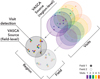 |
Fig. 1 VASCA data model, see main text for more details. |
2 VAriable Source Cluster Analysis pipeline
VASCA offers a modular and scalable analysis pipeline for creating catalogs of cosmic variables from repeated photometric observations. The pipeline is implemented in an instrument-independent manner. We describe it in the following sections using the GALEX dataset as a hands-on application.
2.1 Data model and the GALEX dataset
VASCA is based on a data model that describes photometric detections from repeated observations. These are referred to as “visits” hereafter. A set of visits observing the same patch in the sky in the same passband defines a “field”. A collection of fields defines a “region,” as shown in Fig. 1. Fields can also be overlapping, as in fact is often the case for instruments that perform surveys and follow-up observations. The data model is kept simple by only defining these three hierarchical data layers. It should be noted that observations in different passbands and by different instruments are treated as separate fields, even if they observe the same patch of the sky. Fields are combined only at the region level. This is fundamentally the reason for the pipeline’s scaling ability and instrument independence.
We applied VASCA to 385 NUV fields and 270 FUV fields of the GALEX legacy data on the Multimission Archive at STScI (MAST). These fields fulfilled the following conditions: (1) they had been visited at least ≥ 10 times in the NUV band, and (2) the average NUV exposure is >800s. We applied our selection to the NUV band only, as FUV-only data were very rarely captured by GALEX. The number of visits in the NUV band for each considered field in the sky is shown in Appendix A. The average number of visits for each field is 26.6 in the NUV and 18.9 in the FUV. The total exposure is 12.5 Ms in the NUV band and 5.9 Ms in the FUV band. This is approximately 7.7 times the exposure of the TDS. The applied selection ensures a rather uniform dataset, with an average exposure time per visit of 1.220 s. The average limiting fluxes at a signal-to-noise ratio of three for a typical visit are therefore fNUV ≈ 2.0 µJy and ƒFUV ≈ 2.2 µJy ( , respectively).
In this work, we used GALEX Release 6/7 data products. A description of this standard pipeline and calibration can be found online3 and in Morrissey et al. (2007). NUV- and FUV-band photometry is provided in these data products. The systematic flux accuracy of the pipeline photometry is expected to be 0.8% and 2.5% on average for the NUV and FUV bands, respectively.
We cross-checked the accuracy of the photometric measurements by comparing the observed flux variations with those expected for the measured flux errors. To avoid the inclusion of strongly variable sources into the dataset, we only considered sources with aχ2 probability to a constant flux PVALflux > 0.001 and more than five light-curve points. As shown in Fig. 2, the difference between the observed variations and those expected from the measured errors is <10% and <20% in the NUV and FUV bands, respectively. Assuming that the sources are not time-variable within the photometric sensitivity of GALEX, this comparison would yield a measure of GALEX photometry accuracy. However, as low-level variable sources remain in the sample, this corresponds to an upper limit of the stability of flux determination. These limits are in agreement with the systematic errors quoted previously. It should be noted that the discrepancy observed at low-flux levels is a selection effect: only upward-flux fluctuations are detected close to the flux sensitivity threshold.
The GALEX images contain several different artifacts, and a detailed discussion can be found in Million et al. (2023). These artifacts can create artificial sources or source variability. To minimize their effect in our pipeline, we performed stringent quality cuts on the photometric detections. In particular, selection cuts were applied to ensure that only point-like sources were selected, as artifacts are typically extended and asymmetric. Furthermore, we restricted our analysis to the inner camera, where artifacts are sparser. Finally, we required a minimum of three independent detections for each source, as artifacts typically do not repeat in position over multiple visits. All selection variables and values are listed in Table 1.
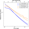 |
Fig. 2 Comparison of the flux variations observed in VASCA sources and photometric measurement errors for NUV (blue lines) and FUV (red lines) passbands. See text for further details. |
Selection parameters used in the VASCA pipeline.
2.2 Pipeline and variability selection
A schematic representation of the VASCA analysis flow is shown in Appendix B. The photometric detections of each visit are inputs to the pipeline. After quality selection, detections were clustered for all visits of each field using the mean-shift algorithm (Pedregosa et al. 2011; Comaniciu & Meer 2002). The clustering bandwidth is always fixed at 4″, which is significantly larger than the typical absolute astrometric performance of ⪅1.5″ of GALEX (Morrissey et al. 2007).
A second clustering was performed for all clusters obtained in the field analysis to take into account different observation filters and overlapping fields. The clusters obtained in this second step defined the position of the 1UVA source. The position and mean flux were calculated as the error-weighted mean of all detections associated with the individual cluster. For GALEX observations, additional source photometry was typically provided for the sum of all visit images in a field, the so-called co-added image. This information was also fed into the pipeline. Co-added image detections were clustered and associated with the sources previously derived from the visit detections.
Statistical measures were calculated to diagnose source time variability. The primary statistic for a constant flux is the χ2 probability. We selected sources that were incompatible with a constant flux at the 5-σ level. We also selected sources with a significant difference between the mean flux and the co-added flux. The former is defined as the error-weighted mean of the flux in all visit-level detections, whereas the latter is obtained from the photometry of the co-added images. This cut was applied to select sources that were only detected during bright flaring periods in a few visits. All selection values are listed in Table 1. To consider possible systematic flux variations, we also selected the normalized excess variance of the flux,  , where Varflux and errflux are the variance and error of the flux measurements (Vaughan et al. 2003). The selection of the minimum excess variance corresponds to a flux variability of ≈3% and ≈10% for the NUV and FUV bands, respectively. This is approximately four times the expected photometric stability of GALEX discussed in the previous section, ensuring that no instrumental variations lead to artificial variability.
2.3 Source association
To find multi-frequency counterparts, we checked for positional coincidences within 1.5″ for all 1UVA sources. This match was performed for all sources listed in the Set of Identifications, Measurements, and Bibliography for Astronomical Data (SIMBAD) database (Wenger et al. 2000), the Gαiα-DR3 and WD catalogs (Gaia Collaboration 2023; Gentile Fusillo et al. 2021) and the recent GALEX Flare Catalog (Million et al. 2023). The latter lists sources in GALEX data that are variable within one visit. In the case of multiple counterparts in one catalog, the closest one was taken.
To obtain a spectral energy distribution (SED), we used the VizieR photometry tool4. This provides all SED points from all entries in the VizieR database (Ochsenbein et al. 2000). We caution that the latter was done without specific checks on the quality of these catalogs. Finally, we also queried whether spectra from the Sloan Digital Sky Survey were available for each source (Abdurro'uf et al. 2022).
2.4 Periodicity search
We performed a periodicity search using a Lomb-Scargle peri-odogram (Lomb 1976; Scargle 1982) in the frequency range of 0.03 d−1 to 2d−1. For all 1UVA sources, we estimated the significance of the main peak in the periodograms using Baluev’s method Baluev (2008). We included periodicity frequency peaks with a significance greater than 4-σ in the catalog if the light curve contained more than 20 points. We are aware that the use of these periodicity detection methods has significant caveats in the case of sparse binning, as is typically the case for light curves in the catalog (for a discussion, see e.g., VanderPlas 2018). We therefore considered the reported periodicities as provisional. They may prove useful for future investigations into periodicity among these sources, especially when utilizing more uniformly sampled light curves.
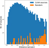 |
Fig. 3 Angular distance between 1UVA sources and associated Gaia-DR3 sources for the source positions measured (blue bars) and randomly scattered positions (orange bars). |
3 Catalog of ultraviolet variable sources
In total, our pipeline found 1991 105 UV sources. Of these, 4202 sources passed the flux variability selection. The latter composes the 1UVA catalog. A list of the information available for each source in the catalog is provided in Appendix C. On average, the light curves of 1UVA sources contain 6.1 photometric measurements in the NUV and 3.4 in the FUV passbands. A wide range of timescales was probed, from ≈90 min to ≈8 yr. The distribution of time differences between the light-curve points is shown in Appendix A.
We found multi-frequency counterparts for 3656 sources: 3301 sources have a counterpart in the Gaia-DR3 catalog and 2686 sources have a counterpart in the SΓMBAD database. The distance distribution between the 1UVA positions and the associated Gaia-DR3 sources is shown in Fig. 3. The average angular distance is 0.40″. As the positional uncertainties of Gaia-DR3 sources are negligible compared to those of GALEX, this also corresponds to the mean positional accuracy of the 1UVA sources.
To check the chance probability of false associations, we shifted the 1UVA source positions randomly between 2 to 60″ five times and performed the source association again; on average, only 14.8 Gaia-DR3 associations were found; their distance distribution is shown in Fig. 3. The small number of random matches confirmed the expectation that only a few sources in the catalog were wrongly associated. This further confirms that only a minor fraction of spurious sources, if any, are included in the 1UVA catalog.
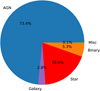 |
Fig. 4 Object groups for 1UVA counterpart sources with a secured source type in the SIMBAD database. See Table 2 for further details on subdivisions. |
3.1 Source classes
To classify the types of 1UVA sources, we relied on the classification used in the SIMBAD database5. The distribution of source types is shown in Fig. 4 and listed in more detail in Table 2. Both show only SIMBAD counterpart sources with a secured source type.
In general, a large diversity of sources was found. As expected, the vast majority of sources are AGN (≈73%). Among these, the subclass of quasars dominated the sample. The second largest class of sources are stars, either single (≈18%) or in binary systems (≈5%). Non-active galaxies (≈2.8%) and one HII region were also found; these large, diffuse objects must contain a variable source within them, the type of which remains unknown at this point.
In two cases, 1UVA sources were associated with an SN explosion. In the first case, 1UVA J141829.9+534331.0, the time profile corresponds to the SN PSl-llpf (Sanders et al. 2015). In the second case, 1UVA J33308.1-271452.5, the observed UV variability precedes the associated “SN cdfsl r 20121007 43A” by several years. In addition, the latter is classified as “probably supernova” in the original catalog (Cappellaro et al. 2015). This source is therefore very likely not a SN.
The square root of the flux-excess variance of the different source classes for the NUV and FUV bands is shown in Fig. 5. In both bands, the observed variability amplitude varies between a few percent to a factor of approximately ten. The variability amplitude is generally larger and extends to higher values for stellar objects than that for AGNs. A similar trend was observed in the TDS survey (Gezari et al. 2013).
Due to the richness of the dataset, a deeper study of all source types found in the 1UVA catalog is beyond the scope of this article. Here, we focus on two findings: first, the large variety of stars found in the 1UVA catalog; and second, the two WDs that were found to be variable, although their SEDs do not indicate the presence of any companion star. We subsequently go into more detail on both findings in the following sections.
Types of 1UVA counterparts in the SIMBAD database.
3.2 UV-variable stars
As can be seen in Table 2, many different stellar classes are found to be UV-variable. As expected from previous studies, the dominant class is RR Lyrae stars (Gezari et al. 2013). Several other pulsating stars were also observed, such as pulsating variables, Cepheids, and Delta Scuti variables. Perhaps more surprisingly, 20 high-proper-motion stars were found in the sample.
Using the Gaia-DR3 associations, we constructed the Hertzsprung-Russel (HR) diagram of the Gaia counterparts of 1UVA sources, shown in Fig. 6. The figure also shows the star density for a random sample of Gaia sources. For both, we applied the same quality cuts on the Gaia measurements; the signal-to-noise ratios for both the blue and red filter photometry, as well as the parallax measurements, all exceeded ten. The fluxes of sources beyond 150 pc were corrected for dust extinction using estimates from the low-resolution Gaia spectra (Andrae et al. 2023). Only sources for which the latter extinction estimate was available were included in the sample. In addition, sources were only included if they had an extinction in the G band AG < 1. All sources within a distance of 150 pc were included without correction for extinction, as we anticipated it to have a minimal effect in the scenario AG ≲ 0.02.
It is interesting to note that 1UVA sources are found throughout the HR diagram, although there is a strong selection bias toward bluer stars due to the UV selection of the sample. UV variability seems to be ubiquitous for stars, regardless of whether they are on the main sequence or in the horizontal branch. In the former, a shift toward redder and brighter sources is seen for stars with absolute magnitudes larger than approximately seven. This is likely due to the fact that UV variable sources are generally binary systems (Gaia Collaboration 2018). Finally, WDs were also found in the sample.
3.3 UV-variable white dwarfs
White dwarfs are known to exhibit significant variability in the UV spectrum when they have a stellar companion. The accretion of matter from the companion star can lead to strong nova explosions in cataclysmic variables (CVs Inight et al. 2023). Eleven CV counterparts were indeed found for 1UVA sources in the SIMBAD database (see Table 2). Time variability has also been found for WDs with substellar companions; obscuration during eclipses and the heating of the companion can cause flux periodicity on timescales between a few hours and several days (Hernandez Santisteban et al. 2016; van Roestel et al. 2021). On short timescales of ≈10 min, periodic UV variability has been found for isolated WDs from their rotating photosphere in so-called pulsators (Rowan et al. 2019).
We searched for isolated variable WDs among the 1UVA sources. For this, we selected sources with counterparts classified as WDs at >90% confidence in the Gaia-EDR3 WD catalog. The properties of the four 1UVA counterpart sources that passed these selection criteria are listed in Table 3. It should be noted that this classification is more reliable than that of the SIMBAD database used previously. Two sources that had been classified as WDs in the SIMBAD database did show a probability <35% of being a WD in the Gaia-EDR3 WD catalog (1UVA J234829.1–92500.3 and 1UVA J221409.9+05246.0). These were therefore not included in this discussion.
The SEDs of these sources are shown in the left panels of Fig. 7. No companion star is visible in any of the cases. To emphasize this point, we included the SED of a putative dim brown dwarf star companion in the SED in this figure. The star was assumed to have a radius of 0.1 R⊙ and a temperature of 2700K. As evident, the measured fluxes are roughly one order of magnitude lower than the anticipated stellar emission, particularly in the infrared region.
The UV light curve of the four WDs is shown in the right panels of Fig. 7. All of these exhibit variability. The timescale of this variability must exceed the typical observation duration of ≈ 24 min. In several cases, there are signs of long-term trends spanning from days to years. For example, in the case of WD J004917.14–252556.81, all flux measurements from 2009 are lower than those recorded in 2004. However, given the limited data available, these trends may be due to the random sampling of shorter-term variability.
One of the sources, WD J221828.58–000012.17, is classified as a magnetic WD. Flux variations from magnetic WDs are well documented (Lawrie et al. 2013): they are caused by the WD’s rotation and typically occur over periods ranging from several minutes to several days. The typical amplitude of these flux variations, measured from peak to peak, is a few percent. However, due to the limited availability of UV data, no periodicity can be discerned, potentially explaining the observed flux variations for this source.
Two other sources, WD J004917.14–252556.81 and WD J022222.85–005026.59, are classified as normal DA WDs. Variability with timescales ≳ 24 min is atypical for these sources, and may suggest ongoing accretion from an undetected substellar companion. However, no companion was seen in the SED and no spectral lines indicating an accretion disk were observed in the optical to infrared spectrum (Kilic et al. 2023b). Periodic absorption of light by planetary debris orbiting the WD is another possibility (Vanderbosch et al. 2020). A third possibility might be that the temperature of the photosphere is fluctuating due to an as-yet-unknown reason.
WD J004917.14–252556.81 is of particular interest, as pulsations with periods of TP1 = 221.36 s and TP2 = 209.3 s have been detected from this source (Kilic et al. 2023a). The peak-to-peak amplitude of these pulsations is ≈30%. This source is the most massive WD to exhibit pulsations observed to date. We conducted a search for these periodic signals in the GALEX data and derived a light curve sampled in 40 s bins using the gPhoton tool (Million et al. 2016). We found that this is the smallest time binning at which the photon count rate per bin remains within acceptable limits. Unfortunately, this time binning does not allow us to resolve the periods TP1 and TP2 separately.
As the WD oscillations may shift with time (Kilic et al. 2023a), we conducted a Lomb Scargle test to search for periodicities in the GALEX data for four observing blocks: MJD 52925.31975–52925.61277, 55096.10218–55097.06439, 55104.57558–55106.78567, and 55123.12991–55128.62543. The periodogram is given in Appendix D. No significant pulsations were detected in all observing blocks, except for the third. In this particular block, a peak was observed in the periodogram at TP = ≈218 s with a false probability of 0.10%. This period is in agreement with TP1 and TP2 within the accuracy of our data’s time binning. We therefore interpret this as an indication that the observed oscillations also manifest in the UV, at least during certain intervals. To definitively address this question, more sensitive UV observations with finer time resolution will be required.
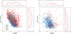 |
Fig. 5 Flux vs. the relative amplitude of flux variations given by the square root of the normalized excess variance as a function of the mean flux for the NUV (left) and FUV (right) passbands. The axis ranges have been kept the same in both bands to facilitate comparison. The subpanels at the top and right of each image show the total number of sources projected onto the respective axis. |
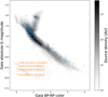 |
Fig. 6 Hertzsprung-Russel (HR) diagram for VASCA sources with Gaia-DR3 counterparts (blue points, see text). The gray background map shows the source density of randomly selected Gaia-DR3 sources for comparison. Gaia source selection cuts are identical in both cases. The orange marker shows the UV-variable WDs discussed in Sect. 3.3. |
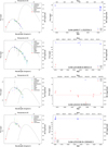 |
Fig. 7 SED (left) and light curve (right) for the sources listed in Table 3. Left: the straight line shows the best fit to a blackbody emission spectrum. The blackbody temperature is given in Table 3. The dashed line shows the SED of a brown dwarf star in a blackbody approximation (see main text). Right: the dashed line shows the mean flux value. |
4 Summary and outlook
We present here the 1UVA source catalog of variable UV sources. We describe a novel analysis pipeline, named VASCA, designed for clustering and assessing sources identified in photometric data. Utilizing the VASCA pipeline on GALEX data, we identified 4202 variable UV sources exhibiting variability across timescales ranging from ≈30min to several years. We found a multi-frequency counterpart for 3655 of these sources. As expected, AGNs comprises the majority of the source sample in terms of numbers. Variable stars constitute the second largest group.
We found that UV variability is ubiquitous in stellar objects, including those not within binary systems; thus, UV-variable stars are distributed across all regions of the HR diagram. We then focused on WDs that are not in CV systems and found four variable WDs. One of them, WD J004917.14–252556.81, is particularly interesting. This source has recently been found to be the most massive WD with seismic periodic oscillations (Kilic et al. 2023a). We found indications of these pulsations also in the GALEX UV data. The observed UV variability from this source is puzzling, leading us to speculate on several possible scenarios.
Due to its modular design and instrument independence, VASCA can be applied to different surveys in the future. The only requirement is the availability of photometric measurements at the visit level prior to data co-addition. Such data are expected to become available from the upcoming ULTRA-SAT mission (Shvartzvald et al. 2024), the Vera Rubin telescope (Ivezić et al. 2019), and the Cherenkov Telescope Array (Actis et al. 2011) data. For future UV data, the 1UVA catalog offers a long-term reference point for investigating UV flux variability over several decades.
Finally, it should be pointed out that given the extensive data within the 1UVA dataset, our current study could only concentrate on selected sources. We encourage the usage of the VASCA code and the catalog data products for further studies.
Acknowledgements
We thank Thomas Kupfer for insightful discussion on the presented work. This work made use of Astropy (Astropy Collaboration 2022), scikit-learn (Pedregosa et al. 2011), the SIMBAD database (Wenger et al. 2000) and the VizieR catalogue access tool (DOI: 10.26093/cds/vizier).
Appendix A GALEX observations
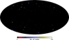 |
Fig. A.1 Number of visits with NUV exposure for each field considered in the 1UVA catalog. The sky map is shown in galactic coordinates in a Mollweide projection. |
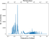 |
Fig. A.2 Time difference distribution between all combinations of light-curve points for the 1UVA sources. |
Appendix B VASCA processing flow
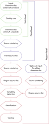 |
Fig. B.1 Schematic of the VASCA processing flow. |
Appendix C Catalog tables content
Columns of the “SOURCES” table of the 1UVA catalog.
Tables from the 1UVA catalog.
Appendix D Periodogram of White Dwarf J004917.14-252556.81
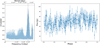 |
Fig. D.1 Periodicity search for WD J004917.14-252556.81. The search was performed on the UV light curve in a 40-second time binning, restricted to the time range between MJD 55104.57558-55106.78567. Left: Lomb Scargle periodogram. Dashed horizontal lines indicate the 2 and 3 σ confidence levels calculated using Baluev (2008). Vertical dotted lines indicate the periods previously found for this source (Kilic et al. 2023a). For more information, see the main text. Right: Phased light curve with the best-fit model (straight line). |
References
- Abbott, B. P., Abbott, R., Abbott, T. D., et al. 2017, ApJ, 848, L12 [Google Scholar]
- Abdollahi, S., Ackermann, M., Ajello, M., et al. 2017, ApJ, 846, 34 [NASA ADS] [CrossRef] [Google Scholar]
- Abdurro’uf, Accetta, K., Aerts, C., et al. 2022, ApJS, 259, 35 [NASA ADS] [CrossRef] [Google Scholar]
- Actis, M., Agnetta, G., Aharonian, F., et al. 2011, Exp. Astron., 32, 193 [NASA ADS] [CrossRef] [Google Scholar]
- Andrae, R., Fouesneau, M., Sordo, R., et al. 2023, A&A, 674, A27 [CrossRef] [EDP Sciences] [Google Scholar]
- Astropy Collaboration (Price-Whelan, A. M., et al.) 2022, ApJ, 935, 167 [NASA ADS] [CrossRef] [Google Scholar]
- Baluev, R. V. 2008, MNRAS, 385, 1279 [Google Scholar]
- Bellm, E. C., Kulkarni, S. R., Graham, M. J., et al. 2019, PASP, 131, 018002 [Google Scholar]
- Bianchi, L., Conti, A., & Shiao, B. 2014, Adv. Space Res., 53, 900 [Google Scholar]
- Bühler, R., & Blandford, R. 2014, Rep. Progr. Phys., 77, 066901 [CrossRef] [Google Scholar]
- Cappellaro, E., Botticella, M. T., Pignata, G., et al. 2015, A&A, 584, A62 [NASA ADS] [CrossRef] [EDP Sciences] [Google Scholar]
- Comaniciu, D., & Meer, P. 2002, IEEE Trans. Pattern Anal. Mach. Intell., 24, 603 [CrossRef] [Google Scholar]
- Cordes, J. M., & Chatterjee, S. 2019, ARA&A, 57, 417 [NASA ADS] [CrossRef] [Google Scholar]
- Gaia Collaboration (Babusiaux, C., et al.) 2018, A&A, 616, A10 [NASA ADS] [CrossRef] [EDP Sciences] [Google Scholar]
- Gaia Collaboration (Vallenari, A., et al.) 2023, A&A, 674, A1 [NASA ADS] [CrossRef] [EDP Sciences] [Google Scholar]
- Gentile Fusillo, N. P., Tremblay, P. E., Cukanovaite, E., et al. 2021, MNRAS, 508, 3877 [NASA ADS] [CrossRef] [Google Scholar]
- Gezari, S. 2021, ARA&A, 59, 21 [NASA ADS] [CrossRef] [Google Scholar]
- Gezari, S., Martin, D. C., Forster, K., et al. 2013, ApJ, 766, 60 [NASA ADS] [CrossRef] [Google Scholar]
- Hernandez Santisteban, J. V., Knigge, C., Littlefair, S. P., et al. 2016, Nature, 533, 366 [NASA ADS] [CrossRef] [Google Scholar]
- Inight, K., Gänsicke, B. T., Breedt, E., et al. 2023, MNRAS, 524, 4867 [NASA ADS] [CrossRef] [Google Scholar]
- Ivezić, Ž., Kahn, S. M., Tyson, J. A., et al. 2019, ApJ, 873, 111 [Google Scholar]
- Kilic, M., Córsico, A. H., Moss, A. G., et al. 2023a, MNRAS, 522, 2181 [NASA ADS] [CrossRef] [Google Scholar]
- Kilic, M., Moss, A. G., Kosakowski, A., et al. 2023b, MNRAS, 518, 2341 [Google Scholar]
- Kulkarni, S. R., Harrison, F. A., Grefenstette, B. W., et al. 2021, arXiv e-prints [arXiv: 2111.15608] [Google Scholar]
- Lawrie, K. A., Burleigh, M. R., Brinkworth, C. S., et al. 2013, in 18th European White Dwarf Workshop., eds. J. Krzesinski, G. Stachowski, P. Moskalik, & K. Bajan, Astronomical Society of the Pacific Conference Series, 469, 429 [NASA ADS] [Google Scholar]
- Lo, K. K., Farrell, S., Murphy, T., & Gaensler, B. M. 2014, ApJ, 786, 20 [NASA ADS] [CrossRef] [Google Scholar]
- Lomb, N. R. 1976, Ap&SS, 39, 447 [Google Scholar]
- Million, C., Fleming, S. W., Shiao, B., et al. 2016, ApJ, 833, 292 [NASA ADS] [CrossRef] [Google Scholar]
- Million, C. C., Clair, M. S., Fleming, S. W., Bianchi, L., & Osten, R. 2023, ApJS, 268, 41 [CrossRef] [Google Scholar]
- Morrissey, P., Conrow, T., Barlow, T. A., et al. 2007, ApJS, 173, 682 [Google Scholar]
- Ochsenbein, F., Bauer, P., & Marcout, J. 2000, A&AS, 143, 23 [NASA ADS] [CrossRef] [EDP Sciences] [Google Scholar]
- Pedregosa, F., Varoquaux, G., Gramfort, A., et al. 2011, J. Mach. Learn. Res., 12, 2825 [Google Scholar]
- Rowan, D. M., Tucker, M. A., Shappee, B. J., & Hermes, J. J. 2019, MNRAS, 486, 4574 [Google Scholar]
- Sanders, N. E., Soderberg, A. M., Gezari, S., et al. 2015, ApJ, 799, 208 [NASA ADS] [CrossRef] [Google Scholar]
- Scargle, J. D. 1982, ApJ, 263, 835 [Google Scholar]
- Shvartzvald, Y., Waxman, E., Gal-Yam, A., et al. 2024, ApJ, 964, 74 [NASA ADS] [CrossRef] [Google Scholar]
- Thyagarajan, N., Helfand, D. J., White, R. L., & Becker, R. H. 2011, ApJ, 742, 49 [NASA ADS] [CrossRef] [Google Scholar]
- van Roestel, J., Kupfer, T., Bell, K. J., et al. 2021, ApJ, 919, L26 [NASA ADS] [CrossRef] [Google Scholar]
- Vanderbosch, Z., Hermes, J. J., Dennihy, E., et al. 2020, ApJ, 897, 171 [Google Scholar]
- VanderPlas, J. T. 2018, ApJS, 236, 16 [Google Scholar]
- Vaughan, S., Edelson, R., Warwick, R. S., & Uttley, P. 2003, MNRAS, 345, 1271 [Google Scholar]
- Wenger, M., Ochsenbein, F., Egret, D., et al. 2000, A&AS, 143, 9 [NASA ADS] [CrossRef] [EDP Sciences] [Google Scholar]
- Zhan, H. 2018, in 42nd COSPAR Scientific Assembly, 42, E1.16-4-18 [Google Scholar]
- Zhu, W., & Dong, S. 2021, ARA&A, 59, 291 [NASA ADS] [CrossRef] [Google Scholar]
All Tables
All Figures
|
Fig. 1 VASCA data model, see main text for more details. |
| In the text | |
|
Fig. 2 Comparison of the flux variations observed in VASCA sources and photometric measurement errors for NUV (blue lines) and FUV (red lines) passbands. See text for further details. |
| In the text | |
|
Fig. 3 Angular distance between 1UVA sources and associated Gaia-DR3 sources for the source positions measured (blue bars) and randomly scattered positions (orange bars). |
| In the text | |
|
Fig. 4 Object groups for 1UVA counterpart sources with a secured source type in the SIMBAD database. See Table 2 for further details on subdivisions. |
| In the text | |
|
Fig. 5 Flux vs. the relative amplitude of flux variations given by the square root of the normalized excess variance as a function of the mean flux for the NUV (left) and FUV (right) passbands. The axis ranges have been kept the same in both bands to facilitate comparison. The subpanels at the top and right of each image show the total number of sources projected onto the respective axis. |
| In the text | |
|
Fig. 6 Hertzsprung-Russel (HR) diagram for VASCA sources with Gaia-DR3 counterparts (blue points, see text). The gray background map shows the source density of randomly selected Gaia-DR3 sources for comparison. Gaia source selection cuts are identical in both cases. The orange marker shows the UV-variable WDs discussed in Sect. 3.3. |
| In the text | |
|
Fig. 7 SED (left) and light curve (right) for the sources listed in Table 3. Left: the straight line shows the best fit to a blackbody emission spectrum. The blackbody temperature is given in Table 3. The dashed line shows the SED of a brown dwarf star in a blackbody approximation (see main text). Right: the dashed line shows the mean flux value. |
| In the text | |
|
Fig. A.1 Number of visits with NUV exposure for each field considered in the 1UVA catalog. The sky map is shown in galactic coordinates in a Mollweide projection. |
| In the text | |
|
Fig. A.2 Time difference distribution between all combinations of light-curve points for the 1UVA sources. |
| In the text | |
|
Fig. B.1 Schematic of the VASCA processing flow. |
| In the text | |
|
Fig. D.1 Periodicity search for WD J004917.14-252556.81. The search was performed on the UV light curve in a 40-second time binning, restricted to the time range between MJD 55104.57558-55106.78567. Left: Lomb Scargle periodogram. Dashed horizontal lines indicate the 2 and 3 σ confidence levels calculated using Baluev (2008). Vertical dotted lines indicate the periods previously found for this source (Kilic et al. 2023a). For more information, see the main text. Right: Phased light curve with the best-fit model (straight line). |
| In the text | |
Current usage metrics show cumulative count of Article Views (full-text article views including HTML views, PDF and ePub downloads, according to the available data) and Abstracts Views on Vision4Press platform.
Data correspond to usage on the plateform after 2015. The current usage metrics is available 48-96 hours after online publication and is updated daily on week days.
Initial download of the metrics may take a while.