| Issue |
A&A
Volume 687, July 2024
|
|
|---|---|---|
| Article Number | A305 | |
| Number of page(s) | 19 | |
| Section | Catalogs and data | |
| DOI | https://doi.org/10.1051/0004-6361/202449358 | |
| Published online | 30 July 2024 | |
Cataclysmic variables around the period-bounce: An eROSITA-enhanced multiwavelength catalog★
1
Institut für Astronomie und Astrophysik, Eberhard-Karls Universität Tübingen,
Sand 1,
72076
Tübingen,
Germany
e-mail: This email address is being protected from spambots. You need JavaScript enabled to view it.
2
Leibniz-Institut für Astrophysik Potsdam (AIP),
An der Sternwarte 16,
14482
Potsdam,
Germany
Received:
26
January
2024
Accepted:
12
June
2024
Abstract
Context. Cataclysmic variables (CVs) with degenerate donors that have evolved past the period minimum are predicted to make up a great portion of the CV population, namely, between 40% and 80%. However, either due to shortcomings in the models or the intrinsic faintness of these strongly evolved systems, only a few of these so-called “period-bouncers” have been confidently identified thus far.
Aims. We compiled a multiwavelength catalog of period-bouncers and CVs around the period minimum from the literature to provide an in-depth characterization of the elusive subclass of period-bounce CVs that will support the identification of new candidates.
Methods. We combined recently published or archival multiwavelength data with new X-ray observations from the all-sky surveys carried out with the extended ROentgen Survey with an Imaging Telescope Array (eROSITA) on board the Spektrum-Roentgen-Gamma spacecraft (SRG). Our catalog comprises 192 CVs around the period minimum, chosen as likely period-bounce candidates based on reported short orbital periods and low donor mass. This sample helped us establish specific selection parameters, which were used to compile a “scorecard” that rates the likelihood that a particular system is a period-bouncer.
Results. Our “scorecard” correctly assigns high scores to the already confirmed period-bouncers in our literature catalog. It has also identified 103 additional strong period-bounce candidates in the literature that had not previously been classified as such. We established two selection cuts based on the X-ray-to-optical flux ratio (−1.21 ≤ log(Fx/Fopt) ≤ 0) and the typical X-ray luminosity (log(Lx,bol) ≤ 30.4 [erg s−1]) observed from the eight period-bouncers that have already been confirmed with eROSITA data. These X-ray selection cuts led to the updated categorization of seven systems as new period-bouncers, increasing their known population to 24 systems in total.
Conclusions. Our multiwavelength catalog of CVs around the period minimum drawn from the literature, together with X-ray data from eROSITA, has resulted in a ~40% increase in the population of period-bouncers. Both the catalog and “scorecard” we constructed will aid in future searches for new period-bounce candidates. These tools will contribute to the goal of resolving the discrepancy between the predicted high number of period-bouncers and the low number of these systems successfully observed to date.
Key words: catalogs / novae, cataclysmic variables / X-rays: binaries
Full Tables 3 and B.2 are available at the CDS via anonymous ftp to cdsarc.cds.unistra.fr (130.79.128.5) or via https://cdsarc.cds.unistra.fr/viz-bin/cat/J/A+A/687/A305
© The Authors 2024
 Open Access article, published by EDP Sciences, under the terms of the Creative Commons Attribution License (https://creativecommons.org/licenses/by/4.0), which permits unrestricted use, distribution, and reproduction in any medium, provided the original work is properly cited.
This article is published in open access under the Subscribe to Open model. This email address is being protected from spambots. You need JavaScript enabled to view it. to support open access publication.
1 Introduction
Cataclysmic variables (CVs) are interacting compact binaries where a white dwarf (WD) accretes matter from a Roche-lobe filling, late-type donor (Warner 1995). According to Paczynski (1976), CVs are the result of a common envelope (CE) phase in the evolution of the binary, where the envelope of a Roche-lobe filling, more massive primary star expands enough to engulf the companion. The envelope is then ejected from the binary, leaving a post-common envelope binary composed by the evolved core of the primary (now a WD) and a low-mass companion still on the main-sequence. At the end of the CE phase the orbital separation of the binary system has been significantly reduced due to friction in the CE that extracts angular momentum and energy from the system. Once the binary separation is close enough to allow mass transfer onto the WD, the system morphs into a CV.
In terms of evolution, all CVs follow a track from longer orbital periods towards shorter ones driven by angular momentum loss which causes the orbital separation (and thus the orbital period) of the system to decrease (Paczynski 1976, Kolb 1993, Warner 1995). For systems with long orbital periods (Porb> 3 h) the dominant angular momentum loss mechanism according to the “standard model” is magnetic braking, arising from the stellar wind associated with the secondary’s magnetic activity (see e.g. Mestel 1968; Verbunt & Zwaan 1981). The evolution of the CV continues until an orbital period of around 3 h, when the secondary becomes fully convective and (according to the standard model) magnetic braking abruptly stops causing a reduced mass transfer rate in the system. This eventually leads to the secondary detaching from its Roche-lobe (King 1988; Ritter 1991), marking the beginning of the “period gap” (3 h ≲ Porb ≲ h), which contains detached CVs. In the standard model, these CVs lose angular momentum exclusively as a result of gravitational radiation (Spruit & Ritter 1983). At the lower boundary of the gap, the secondary is filling its Roche-lobe once again, thereby allowing for the re-start of mass transfer in the system (Kolb et al. 1998).
According to this paradigm, the system re-emerges from the period gap as a short-period CV with angular momentum loss driven exclusively by gravitational radiation (Paczynski 1976). However, the evolutionary track generated by considering gravitational radiation as the only mechanism of angular momentum loss does not comply with observations. Knigge et al. (2011) showed that in order to reproduce the observed evolution of short-period CVs, the angular momentum loss mechanism has to be around 2.5 times stronger than pure gravitational radiation. The origin and nature of this enhanced mechanism for angular momentum loss in short-period CVs is a topic of active discussion, with a wide variety of “recipes” having been suggested (Politano 1996; Zorotovic et al. 2011; Wijnen et al. 2015; Belloni et al. 2020). Amongst these proposals, we highlight the empirical model for consequential angular momentum loss (Schreiber et al. 2016), which appears to solve several major disagreements among theory and observations, even though the physical mechanism behind the additional angular momentum loss is unclear.
Both magnetic and non-magnetic systems can be found amongst short-period CVs. Magnetic systems, which make up around one-third of CVs (Wickramasinghe & Ferrario 2000; Pretorius et al. 2013; Pala et al. 2020), can be further categorized depending on the strength of their magnetic field into polars, with 1 B ≥ 10 MG, which suppresses the formation of an accretion disk forcing the accretion flow to follow the magnetic field lines (Cropper 1990), and intermediate polars, with 1 ≤ B ≤ 10 MG and allowing for a vestigial disk to form (Patterson 1994). Meanwhile, accretion remains primarily through the magnetic field lines.
Short-period CVs, below the period gap, continue to evolve towards even tighter orbits until the system reaches a period minimum. At this point the degenerate donor is out of thermal equilibrium due to its mass-loss timescale becoming much shorter than its thermal timescale, causing the donor to stop shrinking in response to mass-loss (King 1988). The donor, not being able to sustain hydrogen burning, becomes a brown dwarf (Howell et al. 2001). This change in internal structure results in the increase of the system’s orbital separation and consequently the CV bouncing back to longer orbital periods. The systems that go through this process of “bounce-back” to longer periods are known as period-bouncers (Patterson 1998).
Even though the presence of a period minimum has always been a defining characteristic of theoretical models describing CV evolution (Paczynski & Sienkiewicz 1983; Howell et al. 2001; Rappaport et al. 1982; Kolb & Baraffe 1999), evidence supporting its existence only came with a Sloan Digital Sky Survey (SDSS) study of CVs by Gänsicke et al. (2009). A period spike at 80 min ≲ Porb ≲ 86 min was observed providing clear evidence of a “pile-up” of systems that are slowly evolving through the period minimum.
One of the key predictions of theoretical models describing CV evolution is that period-bouncers are expected to make-up the majority of the CV population. Fractions between 40% and 80% of all CVs should have evolved beyond the period minimum, depending heavily on the formation and evolution model used as well as the assumptions made about the systems parameters (see e.g., Kolb 1993; Goliasch & Nelson 2015; Belloni et al. 2020). However, from a volume-limited sample study of CVs by Pala et al. (2020) within 150 pc, the observed fraction of period-bouncers is only between 7% and 14%; also, to date there have been fewer than 20 confirmed period-bouncers (see e.g., Patterson et al. 2005b; McAllister et al. 2017; Neustroev et al. 2017; Pala et al. 2018; Schwope et al. 2021; Amantayeva et al. 2021; Kawka et al. 2021; Muñoz-Giraldo et al. 2023). This under-representation may be due to selection biases against period-bouncers, as their defining characteristics of being old and faint CVs with low luminosity and mass transfer make their detection challenging (Patterson 2011).
Several recent studies suggest dwarf novae as the most likely source for the missing population of period-bouncers (see e.g., Uemura et al. 2010, Kimura et al. 2018). These non-magnetic CVs are characterized by the presence of an accretion disk around the WD which can be observationally identified due to the quasi-periodic changes in brightness known as “outbursts” (Meyer & Meyer-Hofmeister 1984). Dwarf novae can be further classified into several sub-classes depending on the behavior of the outbursts. Furthermore, SU UMa systems are characterized for not only exhibiting outbursts, but also superoutbursts which can last up to several weeks (Vogt 1980). An interesting, and useful, property of these superoutbursts is that they are accompanied with the presence of “superhumps” that originate from donor-induced tidal dissipation of an eccentric accretion disk in a 3:1 orbital resonance (Whitehurst 1988; Osaki 1989). The period of these “superhumps”, which is expected to be a few percent longer than the orbital period (Patterson et al. 2005a), has been established to scale with the mass ratio of the system. This makes it an ideal tool for estimating the masses of the individual components in the CV (Patterson et al. 2005a; Kato & Osaki 2013).
The vast majority of SU UMa are located below the period gap, with donors that are usually M-type or later, making it common to describe the overall short-period non-magnetic CV population as SU UMa-type objects (Kato et al. 2009 and further papers in this series). When an SU UMa has been established through observations to have extremely long outburst recurrence times (in the order of years to decades), a very low mass transfer rate (on the order of 10−11 M⊙yr−1), or a low-mass donor, this CV can be further categorized as a WZ Sge system (Patterson et al. 2002; Kato 2015). In brief, WZ Sge-type CVs have usually the shortest orbital periods of the overall non-magnetic CV population and very low mass donors which may be brown dwarfs (Kato 2022). In fact, the majority of systems found in the “period spike” are classified as WZ Sge-type CVs (Gänsicke et al. 2009), which further supports this theory. This has led to the population of already identified WZ Sge-type objects being established as a good source for finding new period-bounce candidates. However, it is important to consider that these objects are detected primarily through photometric studies of optical superoutburst light curves. This means that they are not easily observed in quiescence due to their faintness and, therefore, they have remained largely undetected in other wavelengths, making a straightforward classification as a period-bouncer challenging.
Spectroscopic studies using a variety of instruments including the Hubble Space Telescope (HST) and SDSS (see e.g., Pala et al. 2022, Inight et al. 2023b) are also an important source for period-bounce candidates. Spectra in the ultra-violet (UV) and optical bands in the case of period-bouncers are strongly dominated by the WD, often with no contribution from the late-type donor at all. This introduces new possibilities and challenges in the search for period-bouncers as potential candidates could be found in single WD catalogs (Inight et al. 2023b) in great numbers, but it makes it necessary to distinguish between these systems. Period-bouncers could also be incorrectly categorized as detached binaries, specially considering the low mass transfer rates that they exhibit (Inight et al. 2021; Schreiber et al. 2023). V379 Vir is a confirmed period-bouncer that was initially assumed to be a detached binary (Schmidt et al. 2005); however, it was later proven to be accreting through the detection of orbital modulation from a deep X-ray observations using XMM-Newton (Stelzer et al. 2017).
Considering that coronal X-ray emission is not expected from the very late-type donors of period-bouncers (Audard et al. 2007; De Luca et al. 2020), the detection of X-ray emission is a key diagnostic of ongoing mass accretion in these systems, which unequivocally distinguishes period-bouncers from isolated WDs and detached binaries, and hence is the most promising path for the identification of new candidates. Even though the high sensitivity of X-ray instruments, such as XMM-Newton, is useful when identifying accreting period-bounce systems, the use of all-sky surveys might be more pertinent for the large-scale search of period-bouncers that is required in order to bring the number of detected systems up to the expected values.
With the launch of the extended ROentgen Survey with an Imaging Telescope Array (eROSITA; Predehl et al. 2021) on board the Spektrum-Roentgen-Gamma mission (SRG; Sunyaev et al. 2021) we gained access to large statistical samples of X-ray sources. The first eROSITA detections of confirmed period-bouncers (Muñoz-Giraldo et al. 2023) proved the capabilities of this instrument in the study and classification of such faint sources. This supports its application as a reliable tool for the identification of new period-bounce candidates. The X-ray study of period-bouncers with eROSITA will help us establish the class properties that will aid in the search for new candidates in the future, with the aim of resolving the discrepancy between observed and predicted fraction of period-bouncers.
The main focus of this study is to produce a catalog of CVs around the period minimum, namely, potential period-bouncers, which were already discussed in the literature, in order to characterize in detail the elusive subclass of period-bounce CVs. To this end, we constructed a literature catalog including both confirmed period-bouncers and candidates. The inclusion of confirmed period-bouncers allows us to use their reported parameters to rate how likely the other candidates are of being a period-bouncer. This catalog will also provide a reliable observational data set that could be used for any future theoretical modelling of advanced CV evolution.
Our literature catalog of period-bounce candidates is introduced in more detail in Sect. 2. We provide specific information in the selection of candidates, followed by an overview of the parameter values used from the literature and comments on the evolution of short-period CVs that can be derived from this information. We wrap up Sect. 2 with a discussion on the quality of the distance values used in the catalog. The process to obtain the photometry of the systems in the catalog is explained in Sect. 3, In Sect. 4 we introduce and explain in detail the scorecard we constructed in order to rate the likelihood a system has of being a period-bouncer. In Sect. 5, we discuss the eROSITA X-ray detections of period-bounce candidates from our catalog and we establish their X-ray characteristics. We present our conclusions in Sect. 6.
2 Literature catalog of period-bounce candidates
We have compiled a catalog of systems already reported in the literature that are characterized by being short-period CVs close to (or already past) the period minimum. This collection of CVs around the period-bounce constitutes an increase in the number of compiled systems of about an order of magnitude compared to earlier studies of period-bounce candidates (Littlefair et al. 2003; Knigge 2006; Gänsicke et al. 2009; Patterson 2011; Inight et al. 2023b). It also provides a comprehensive overview of what is currently known of CVs in the short-period regime.
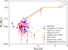 |
Fig. 1 Donor mass as a function of orbital period for the objects in our literature catalog of period-bounce candidates. The color and shape corresponds to the catalogs from which we took the system (and that are listed in the legend). Two CV evolution tracks from Knigge et al. (2011) are shown as reference: the standard track considering angular momentum loss only due to gravitational radiation (blue) and a revised track that considers enhanced angular momentum loss (orange). |
2.1 Candidate selection
We manually went through different databases and individual papers in order to compile a “unified” catalog of potential members of the widely elusive subclass of CVs known as period-bouncers. To this end, we initially selected objects that had a very low donor mass with an orbital period placing them around the period minimum or in the post-bounce area. Additionally, we also included systems that were suggested as good period-bounce candidates even if they either had no reported orbital period/donor mass or their literature parameters did not match our above criteria on donor mass and system orbital period. Examples of this include systems resembling period-bouncers when analysing their spectrum (Inight et al. 2023b), optical light curve (Kimura et al. 2018), WD temperature (Pala et al. 2022), among others, even if their orbital period or donor mass could not be determined probably due to sparse or poor quality data.
The data sources we got most of the systems from are given here, in the order of their dates of publication: Littlefair et al. (2008), Patterson (2011), Otulakowska-Hypka et al. (2016), Kimura et al. (2018), Longstaff et al. (2019), Kato (2022), and Inight et al. (2023b). Henceforth, they are referred to as the “literature catalogs.” Additionally, we also considered systems that were studied individually in dedicated articles (see e.g., Savoury et al. 2012; Beuermann et al. 2021; Kawka et al. 2021; Wild et al. 2022 and Liu et al. 2023). This resulted in a literature catalog of 192 systems, by far the largest data base of period-bounce candidates studied to date.
The vast majority of the systems in our catalog, 133 out of 192 candidates, come from photometric studies of dwarf novae (both SU UMa and WZ Sge-type objects) specifically aimed at the study of superhumps in their superoutbursts (Otulakowska-Hypka et al. 2016, Kimura et al. 2018, Kato 2022). This type of photometric studies are specially relevant for us because they provide a superhump period for a large number of systems that can be used to obtain the mass ratio of the system (see Kato & Osaki 2013 for a comprehensive review of this method), and therefore yields the mass of the donor for a known WD mass.
The location of the 175 systems that have both orbital period and donor mass reported in the literature is presented in Fig. 1 with respect to the period-bounce area predicted from different tracks for the evolution of CVs by Knigge et al. (2011). The error bars presented in Fig. 1 represent the range of donor masses measured for the systems if more than one value was found in the literature. All of the systems except for one, V1258 Cen, populate the area around the period minimum with a sizeable number of them located in the post-bounce area. V1258 Cen was proposed as a period-bouncer by Pala et al. (2022) due to its very low WD temperature, a key characteristic of this type of CV. However, detailed studies of V1258 Cen rule out this system as a period-bouncer, considering that it has an orbital period of 128 min (McAllister et al. 2019) and a donor mass of 0.198 ± 0.029 M⊙ (Savoury et al. 2012) which are too large to belong to a system past the period minimum We decided to keep this system in the catalog in order to compare its characteristics to other systems that are more likely to be period-bouncers. In particular, V1258 Cen may serve as a check to the scorecard that we define in Sect. 4.
Our literature catalog contains 17 “bona fide” period-bouncers. These systems, shown in Table 1, have been classified in the literature as such because they exhibit several key characteristics of period-bouncers in addition to a spectroscopic or photometric confirmation of a late-type donor. These confirmed period-bouncers will be used as a check to the scorecard. In Col. 4 of Table 1, we anticipate the final score for each of them according to the analysis we present in Sect. 4. In our scoring system, a value of 100% is given to systems that have achieved the maximum possible score. Only two of the confirmed period-bouncers reach a 100% score, with a minimum score of 64% which defines the lower boundary we applied to the full catalog, as described in Sect. 4.
2.2 Literature values
We aimed to compile a catalog that has as much information on the period-bounce candidates as possible, including literature values on the following parameters: name, Gaia-DR3 ID, coordinates (J2000), orbital period (Porb), temperature of the WD (Teff), mass of the WD (MWD), WD magnetism type, mass of the donor (Mdonor), spectral type of the donor (SpTdonor), and the Gaia-DR3 distances given by Bailer-Jones et al. (2021). These parameters were drawn for the most part from the literature catalogs listed in Sect. 2.1. In the case where no information was given on some parameters, or an updated value existed, we used additional references to supplement the catalog. A shortened version of our literature catalog is shown in Table B.2 with a brief description of the columns in Table B.1. In the following, we specify how we chose them from the literature.
Orbital period, available for 190 systems. The majority of orbital period values were derived through light curve analysis from optical surveys (see e.g., Otulakowska-Hypka et al. 2016, Kato 2022), with a few of them coming from other methods like radial velocities from Hα emission (see e.g., Breedt et al. 2012, Pala et al. 2018) or X-ray light curves (see e.g., Stelzer et al. 2017, Muñoz-Giraldo et al. 2023). In the specific instances where more than one source had a reported orbital period for a given system, the values were in all cases consistent with each other. In these cases, we chose to keep the value from the most recent derivation.
Donor mass, available for 175 systems. Considering that this parameter has the highest degree of uncertainty as it is rarely measured directly, when possible, we used two values for each object, often determined from different methods. This allowed us to obtain a range for the expected mass of the secondary, illustrated by the error bars in Fig. 1. The majority of the values come from using the WD mass together with the mass ratio (q = Mdonor/MWD) determined by either the superhump method (Kato & Osaki 2013) or the eclipse modeling method (Savoury et al. 2011). If no value for the WD mass was available, we used the value of 0.8 M⊙ determined by Pala et al. (2022) as the mean mass of WDs in CVs.
Spectral type of the donor, available for 38 systems An accurate determination of the SpT is particularly relevant for the study of period-bouncers as the spectral type of the donor –together with its mass –is the parameter that is both the most important and the most difficult to determine precisely in a system with faint, very-low-mass donor. We used the classifications that preferably had a spectroscopic (see e.g., Farihi et al. 2008; Santisteban et al. 2016) or, if not, a photometric confirmation (see e.g., Amantayeva et al. 2021; Kawka et al. 2021).
White dwarf temperature, available for 80 systems. The majority of the values come from UV spectroscopy (Pala et al. 2022) and optical photometry (Gentile Fusillo et al. 2021). When no value was available from either of the methods, we considered temperatures derived from eclipse modeling or evolutionary status (see e.g., McAllister et al. 2019; Savoury et al. 2011).
White dwarf mass, available for 47 systems. The majority of the values come from eclipse modeling (see e.g., Savoury et al. 2011; McAllister et al. 2019) and UV spectroscopy (Pala et al. 2022). When neither value was available, we considered masses derived from gravitational redshift (Neustroev & Mäntynen 2023) or optical spectroscopy (Muñoz-Giraldo et al. 2023).
White dwarf magnetism type, available for 94 systems. From broad sample studies (see e.g., Patterson 2011; Belloni et al. 2020; Pala et al. 2022), which commonly focus on non-magnetic CVs (as they are better understood and expected to follow standard evolution tracks), we categorized the systems present in these studies as non-magnetic. For magnetic CVs, we used individual references that in most cases identified the magnetic nature of the WD from the optical spectra (see, e.g., Breedt et al. 2012; Kawka et al. 2021).
Confirmed period-bouncers in the literature catalog.
2.3 Comments on short-period CVs
Considering that our catalog of short-period CVs has a large population of systems with information about key parameters in CV evolution, we have used this knowledge to comment on the observational characteristics of this type of systems.
2.3.1 Evolution tracks
The evolution of CVs, especially in the short-period regime, is still heavy debated, with theoretical models often clashing with results from observations. This has led to the development of several empirical (or semi-empirical) evolution tracks. Knigge et al. (2011) proposed a semi-empirical donor-based CV evolution track that, in the short-period regime, relies on a mechanism for angular momentum loss that is around 2.5 times stronger than pure gravitational radiation. The difference this change introduces can be easily observed in Fig. 1, where the revised model (orange line) is characterized by a period-bounce area associated with longer orbital periods when compared to the standard theoretical model (blue line). From the 175 systems in our catalog of period-bounce candidates that have a literature value for both the orbital period and the donor mass (shown in Fig. 1), we notice that short-period CVs seem to be located preferentially around the revised Knigge et al. (2011) evolution track. Only a few of the period-bounce candidates reach the short orbital periods associated with the period minimum of the standard evolution track, showing that for a given donor mass this track substantially underestimates the orbital period of the system. Previous CV studies have already noticed that a revised evolution model is necessary to reproduce observations (Littlefair et al. 2008; Pala et al. 2017; 2022; McAllister et al. 2019). However, it is important to note the considerable scatter in the distribution of the systems at or after the period minimum suggesting that the unique track of CV evolution might diverge around the bounce-back area. This scatter has been suggested to be related with the substantial range of masses that the WD may have (Howell et al. 2001) as the WD mass in CVs has been proven to not be constrained by the orbital period (Pala et al. 2022).
2.3.2 WD magnetism
The magnetism of the WD has been considered as a factor that may affect the evolution of CVs, leading to different evolution tracks depending on whether the WD is strongly magnetic or not (Gänsicke et al. 2009; Belloni et al. 2020). In magnetic CVs magnetic braking is expected to be reduced as the wind from the donor may be trapped within the magnetosphere of the WD, causing a difference in the rate of angular momentum loss between magnetic and non-magnetic CVs (Webbink & Wickramasinghe 2002). However, this difference is expected to be significantly reduced for short-period CVs as, in the standard model, gravitational radiation is believed to be the primary mechanism of angular momentum loss in the system with only a weak contribution by magnetic braking (Belloni et al. 2020; Schreiber et al. 2021). The distribution of the 94 systems in our catalog with information about the magnetism of the WD support this scenario, considering that we do not observe an evolution track in Fig. 2 being preferentially populated by either magnetic or non-magnetic CVs.
What we do observe from Fig. 2 is a clear difference between the pre- and post-bounce distribution of the magnetic and non-magnetic CVs. Only two out of the eleven magnetic systems are clearly past the point of period reversal (Mdonor ≈ 0.058 M⊙; Knigge et al. 2011) corresponding to ~ 20% of this population. On the other hand 34 out of 82 non-magnetic systems are located in the period-bouncer area accounting for ~ 40% of this population. This implies that non-magnetic CVs are twice as likely to have evolved past the period minimum than magnetic CVs which might be taken as a hint for longer evolutionary times for magnetic CVs. This falls in line with expectations from simulations, where Belloni et al. (2020) observed a difference of −10% between the number of period-bouncers in magnetic and non-magnetic population, with fewer magnetic CVs managing to become period-bouncers.
The lack of differentiation between evolution tracks of magnetic and non-magnetic CVs, as well as the overrepresentation of magnetic CVs in the pre-bounce area, could also be explained by the low number of observed short-period magnetic CVs, which leads to an incomplete representation of their evolution track. Magnetic CVs in our catalog account for 10% of the population, which is considerably fewer than the expected ~30% (Wickramasinghe & Ferrario 2000; Pretorius et al. 2013; Pala et al. 2020) obtained in previous CV population studies. Rather than showing the true picture of magnetic and non-magnetic short-period CVs, this result evidences a bias of our catalog towards non-magnetic systems. As already discussed in Sect. 2.1 the majority of our candidates are dwarf novae, a type of non-magnetic CV, selected from large photometric studies that provide both orbital period and mass of the systems. Such databases are not as readily available for magnetic systems making their inclusion into our catalog more challenging as we had to rely on individual papers that often did not include all the parameters required. This results in an underrepresentation of magnetic CVs in our catalog of period-bounce candidates.
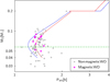 |
Fig. 2 Evolution for magnetic and non-magnetic CVs for the 94 systems in our literature catalog with information about the magnetism of the WD. Point of period reversal (Mdonor ≈0. 058 M⊙) is shown by the green dashed line. The two Knigge et al. (2011) CV evolution tracks from Fig. 1 are shown as reference. |
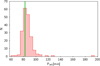 |
Fig. 3 Distribution of the orbital period for 190 systems in our literature catalog with values from the literature. The vertical green line is an estimate of Pspike using a Gaussian fit to the distribution of systems with orbital periods between 77 min and 87 min. |
2.3.3 Period spike and period minimum
The number density of CVs at a given period is inversely proportional to the rate at which the orbital period evolves (Kolb 1993; Kolb et al. 1998; Kolb & Baraffe 1999), making a pile-up or “spike“ of systems at the period minimum an expected characteristic of CV evolution. This was observed for the first time by Gänsicke et al. (2009) using 137 CVs from SDSS. The period “spike“ was established to be located in the orbital period range of 80 min to 86 min corresponding to a significant accumulation of CVs with Pspike = 82.4±0.7 min.
Figure 3 shows the orbital period distribution for 190 period-bounce candidates in our catalog with a literature value. The period “spike“ is observed within the expected range of 80 min to 86 min. We estimated Pspike = 82.4±2.7 min (see green line in Fig. 3) following the description of McAllister et al. (2019) who used a Gaussian fit to the distribution of systems with orbital periods between 77 min and 87min to obtain Pspike = 82.7±0.4 min. Both values are consistent with each other as well as with the Gänsicke et al. (2009) value. Our estimation for Pspike is also consistent with the 81.8±0.9 min period minimum predicted by Knigge et al. (2011) in their revised donor track.
2.4 Distance estimates and limits
To determine the optical properties, and especially the distances, to the systems we performed a match between our literature catalog and the Gaia-DR3 catalog1. Hereby we checked that the resulting match coincided with the Gaia-DR3 ID available in SIMBAD2. Of the 192 systems in our catalog, 159 have available Gaia-DR3 data. 146 of our candidates have Gaia detections at different epochs meaning that they have an available parallax (Gaia Collaboration 2022) that can be used to estimate the distance to the systems.
However, using parallaxes to estimate distances is not a trivial process considering that simply using the inverse of the parallax introduces biases in the distance estimate which affect especially systems with large fractional errors (Bailer-Jones 2015; Luri et al. 2018). As can be seen in Fig. 4, the more distant among the systems from our catalog present large fractional errors, which are greater than 20% for 49 of our period-bounce candidates This is not an unexpected result considering that these systems have on average G ~ 20.1 mag, making their intrinsic faintness, which is characteristic of period-bouncers, the most likely cause for the large uncertainties of their parallaxes (see Fig. 7 from Lindegren et al. 2021).
In order to avoid the introduction of bias into our calculation, which would affect 49 of our candidates with a Gaia parallax value, we chose to use the distance estimates obtained by Bailer-Jones et al. (2021), specifically the geometric distance which takes a probabilistic approach that uses a prior constructed from a three-dimensional (3D) model of our Galaxy to estimate the distances (see Bailer-Jones 2015 for more information on this method). Figure 4 illustrates the difference between both methods used to estimate the distance, showing a significant disagreement for systems at large distances, where the distance from the parallax is underestimated with respect to the distances obtained by Bailer-Jones et al. (2021).
Having an accurate value for the distance is especially relevant for studies like ours considering that many system parameters depend on distance. One example is the magnetic CV EF Eri, which was considered a good period-bounce candidate because at an estimated distance of 111 pc the photometry suggested a brown dwarf donor in the system (Schwope & Christensen 2010). However, once the distance was revised to 160 pc (Bailer-Jones et al. 2021), this argument was not valid anymore disqualifying EF Eri from being a good period-bounce candidate. As EF Eri is included in our literature catalog, we used it similarly to V1258 Cen, namely, as a check of our score card (in Sect. 4).
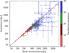 |
Fig. 4 Comparison between the distance obtained by Bailer-Jones et al. (2021) and by using the inverse of the parallax. |
3 Photometry
One possible discriminator between period-bouncers and other CVs regards the IR excess in the composite spectral energy distribution (SED) of the binary system. We include the IR excess as one of the parameters that define our period-bouncer scorecard (Sect. 4). Therefore, we first had to construct the SEDs for the systems from our literature catalog of period-bounce candidates. We used the Tool for OPerations on Catalogues And Tables (TOPCAT3; Taylor 2005) in order to handle our extensive catalog. TOPCAT is a JAVA-based interactive graphical viewer and editor for tabular data that facilities the analysis and manipulation of source catalogues, specially the cross-match between catalogs.
We performed a cross-match in TOPCAT between our catalog and different photometric surveys covering a wide range of wavelengths from ultraviolet (UV) to infrared (IR). When performing the match with the algorithm “sky” we used the right ascension (RA) and declination (DEC) of each system in coordinates J2000, allowing for a match radius of 30″.
We used the following surveys with the latest catalog version available in TOPCAT: Galaxy Evolution Explorer (GALEX) general release GR6+7 (Bianchi et al. 2017); Sloan Digital Sky Survey (SDSS) data release DR16 (Ahumada et al. 2022); UKIRT Infrared Deep Sky Survey (UKIDSS) Large Area Survey data release DR9 (Lawrence et al. 2007); Two Micron All Sky Survey (2MASS) (Skrutskie et al. 2006); VISTA Hemisphere Survey (VHS) data release DR5 (McMahon et al. 2021); Wide-field Infrared Survey Explorer mission (WISE) (Cutri et al. 2021). After obtaining the best matches for each system using a 30″ radius, we carried out a visual check to make sure that there were no other Gaia sources in the vicinity. We discarded those multiwavelength matches that most likely do not belong to our candidate, as they are associated with another Gaia source. This allowed us to obtain an optimal radius with which at least 94% of the correct matches were retrieved and at maximum one incorrect match: 4″ for GALEX (103 correct associations), 4″ for SDSS (82 correct associations), 1″ for UKIDSS (27 correct associations), 2″ for 2MASS (32 correct associations), 3″ for VHS (46 correct associations), and 4″ for WISE (94 correct associations). The multiwavelength photometry we collected this way can be found in the online version of our catalog, with the column descriptions listed in Table B.1.
Using the available photometry for each system, we constructed their individual spectral energy distributions (SEDs), ideally covering wavelengths from UV to IR. These SEDs are used in Sect. 4 to search for an IR excess and to evaluate whether it could be attributed to the presence of a very late-type donor.
4 Period-bouncer likelihood
We used the parameters of the candidates reported in the literature catalog to rate how likely a system is to be a period-bouncer. In this evaluation we considered ten parameters: spectral type of the donor, donor mass, orbital period, WD temperature, photometric colors (UV, optical and IR), optical variability, and IR excess. We compiled them into a scorecard in which we assigned different weights to the parameters depending on how relevant we judged them for confirming a candidate as a period-bouncer. A summary of the parameters and their respective scores is presented in Table 2 and is described in detail below.
4.1 Defining the scoring system
To analyze the likelihood of a system being a true period-bouncer, we assigned numerical scores to each individual parameter that we then combined into a final numerical score for each period-bounce candidate. The values obtained from all individual parameters considered in the scorecard (described in Sect. 4.2) and the final score are reported in Table 3. The maximum number of achievable score points is 36, corresponding to an object that has the highest score in all ten parameters, and hence a final score of 100. However, a considerable number of candidates did not have enough data to be scored in all of the parameters making direct comparison between systems difficult. To solve this problem, for each individual object, we re-define the final score of 100% as the maximum number of points that it would have received if it had the highest likelihood of being a period-bouncer in every parameter for which it has available data. We then calculated the percentage score as the ratio between the actual points the system has and its maximum achievable points. The objects without a percentage value in Table 3 only had available information for three or fewer parameters, which was not enough to characterize such an object as a period-bouncer.
Scores assigned for the different parameters.
Scorecard for the period-bounce candidates in the literature catalog.
4.2 Defining the scorecard parameters & their scores
We present in Table 2 a summary of the scoring system for each parameter and we illustrate this point system with Figs. 5 and 6. Here, the final score achieved by the systems is presented as a color scale and candidates without enough information to have received a final score are presented in yellow. To further enhance the clarity, areas of likelihood are marked by different shape styles: filled circles for high likelihood (three points), crosses for medium high likelihood (two points), triangles for medium likelihood (one point), and squares for low likelihood (zero points). The 17 confirmed period-bouncers from Table 1 are highlighted with black boxes. The assignment of the scores to each parameter is described here in descending order of relevance:
Spectral type of donor. This parameter holds the most weight as spectroscopic detection of a late-type donor in the system is the ultimate confirmation needed to confidently classify a system as a period-bouncer. Period-bouncers are characterized as being CVs with degenerate donors, composed by a WD and either a T dwarf or a L dwarf companion. We also take into account systems with a late M type (M5 or later) as this is indicative of a CV slightly before or just at the bouncing point (Knigge et al. 2011, Kirkpatrick & McCarthy Jr 1994). As was mentioned before, the spectral type of the donor is probably the hardest system parameter to determine in short-period faint CVs. Because of this we decided to award relatively high partial points to systems with a late-M type donor, especially considering that most of them where presented in the literature as a lower limit of the donor spectral type. Even though a spectroscopic detection is the preferred confirmation method for a late-type companion in the system, we also consider photometric data that suggests the presence of a late-type donor in the system.
Donor mass. A very low donor mass is indicative of a highly evolved CV even if there is no direct detection of the donor. In both their standard and revised evolution tracks for CVs, Knigge et al. (2011) obtained a post-bounce area for CVs with a donor mass lower than 0.058 M⊙, this limit is shown as the blue horizontal line in Fig. 5. Systems with slightly higher donor masses (up to a donor mass of 0.07 M⊙ marked by the red line in Fig. 5) would be placed right in the bounce area, meaning that these systems are just within range of being called a potential period-bouncer. When assigning a score to this parameter we considered both possible values for the donor mass if available (see Sect. 2.2 for more information), giving each of the two donor mass values an individual score. For the overall score assigned to a system with two reported values for the donor mass, we considered the average of the two individual scores.
Orbital period. Near the period minimum the orbital period by itself is not a good diagnostic for evolution in CVs. To use Porb as a parameter in the scorecard we consider also the score that each system was given for the donor mass. The clearest example of this are systems with very low donor masses (≤0.058 M⊙ Knigge et al. 2011) for which the orbital period does not have significant incidence as they are all clearly located in the post-bounce area (see filled circles in Fig. 5). For all other systems, their scores are assigned judging their proximity to the observed period minimum of CVs (≈ 80 min; Gänsicke et al. 2009).
WD temperature Considering that period-bouncers are the most evolved systems among CVs, a cool WD temperature (when not in outburst) is expected with temperatures ≤12 500 K (blue line in Fig. 6a; Pala et al. 2022). A temperature higher than 14 000K (red line in Fig. 6a) is no longer reflective of the cool temperature that WDs in period-bouncers are expected to exhibit, and in the rare cases when the measurement was carried out during an outbursts, it should not be considered representative of the true WD temperature.
Gaia variability. As period-bouncers are in the last stage of CV evolution they are expected to be inactive systems with very large recurrence times for both outbursts and superoutbursts in the range of ~ 10 000 days (Patterson 2011). For this reason, unless the period-bouncer is caught in a very rare burst episode, we expect a lack of optical variability. We used the Gaia G-band variability defined in Eq. (1) of Guidry et al. (2021), and defined the selection limits based on the results of Inight et al. (2023a) for WZ Sge-type CVs. According to their Fig. 36 the Gaia variability is≤0.2 for 90% of the objects categorized as WZ Sge in their sample. This threshold is marked by the blue line in Fig. 6b. The Gaia variability of ≤0.3, found for 98% of the objects categorized as WZ Sge in Inight et al. (2023a), are marked by the red line in Fig. 6b. Similar to the WD temperature, this parameter can be affected if the system was undergoing an outburst at the moment of the measurement. For this reason, we also calculated the G-band variability for Gaia-DR2 and assigned a score only for the candidates that received the same score points in Gaia-DR2 and Gaia-DR3, ensuring that their low or high variability is consistent through time and not reflective of sporadic events.
Gaia colors. In optical wavelengths the highly evolved secondary of period-bouncers is not expected to be observable. Therefore, these systems will appear almost identical to an isolated WD (Santisteban et al. 2018). We divided Fig. 6c in the following sectors: a WD locus limited by the blue line (MG ≥ 2.95 × (GBP-GRP) + 10.83; Jiménez-Esteban et al. 2018), a more broadly defined WD locus limited by the blue and red lines (MG ≥ 5 × (GBP-GRP) + 6; Gentile Fusillo et al. 2021), and an area around the main-sequence limited by the red line.
SDSS colors. We aimed to select areas where isolated WDs are expected to be found as the preferential location for period-bouncers. Inight et al. (2023a) plotted a color –color diagram for CVs with SDSS data and reliable photometry (see their Fig. 16) which shows the location of different CV types. We selected the areas where the majority of the Inight et al. (2023a) WZ Sge-type systems were found with 80% of them located between the blue horizontal line (u-g ≤ 0.5) and the blue diagonal line (u-g ≥ 1.25(g-r)-0.1) represented by the filled circles in Fig 6d. 90% of WZ Sge-type CVs are located between the blue horizontal line and the red diagonal line (u-g ≥ 1.25(g-r)−0.4) represented by the triangles in Fig. 6d.
UV colors. For systems in quiescence, GALEX colors are a sensitive probe of the effective WD temperature. Patterson (2011) plotted a sample of dwarf novae (see their Fig. 2) and determined areas where period-bounce candidates are most likely to be found. The area occupied exclusively by period bounce candidates is limited by FUV-NUV ≥ 1 (blue line in Fig. 6e), while the area up to FUV-NUV ≥ 0.25 (red line in Fig. 6e) is populated by period-bounce candidates and other types of CVs. Above the red line in Fig. 6e, Patterson (2011) found no period-bounce candidates.
IR colors. Several regions in the near-IR color –color diagram were identified by Littlefair et al. (2003) depending on the donor type that the population of CVs had (see their Fig. 2). The right part of Fig. 6f is populated by systems with donors identified as either T-type (bottom right) or L-type (top right), while M-type donors are found towards the center (see triangles in Fig. 6f). Earlier type donors and other unidentified donor types are found towards the left part of Fig. 6f, limited by J-H ≤ 3(H-K)−0.6 (red line in Fig. 6f). Littlefair et al. (2003) selected systems with J – H ≤ 3(H – K)−0.8 (blue line in Fig. 6f) as candidates for having a degenerate donor.
IR excess Throughout the evolution of a CV, the companion star loses so much mass that an originally early-type donor, with larger IR contributions, develops into a late-type or degenerate donor that barely contributes to the IR emission of the system. Due to the evolved nature of the secondary in period-bouncers, this very low mass donor is expected to appear as a very slight or no excess in the IR. We constructed SEDs for the 98 candidates that have enough photometric data, and compared them to WD models of spectral type DA with pure hydrogen atmosphere (Koester 2010) using the Virtual Observatory SED Analyzer (VOSA, Bayo et al. 2008). The main takeaway from this comparison is the wavelength at which the IR excess sets in. From the population of 17 confirmed period-bouncers we can establish that this type of CVs, especially the systems that have evolved back to periods larger than 90 min, presents IR excess (from the donor) that starts at relatively long wavelengths associated with the K-band or the WISE bands, if they present an excess at all. Systems close or at the bounce point will have an excess starting at shorter wavelengths associated with the J-band (Owens et al. 2023). Pre-bounce CVs are characterized by larger excess starting at shorter wavelengths (Girven et al. 2011). In Appendix C we show three SEDs that are representative of the different types of IR excess described above.
In Table 3, we show the scorecard ratings for the period-bounce candidates in the literature catalog. Overall, 49 of the 192 systems had information for only three or fewer parameters. As explained above, we did not assign a score to them and we exclude them from the following analysis.
Using the final scores of the 17 systems that have been confidently categorized as period-bouncers and have a spectroscopically confirmed late-type donor (see Table 1), we establish that an object has a high likelihood of being a period-bouncer if its final score is higher than 60%, considering that the confirmed period-bouncer with the lowest score is V406 Vir with 64%. We further divided the remaining candidates as having: medium-high likelihood (between 45% and 60%), medium-low likelihood (between 30%) and low likelihood (lower than 30% for EF Eri these systems are correctly categorized as objects with low and medium-low likelihood of being a period-bouncer respectively. This confirms that our scorecard is functioning satisfactorily as it not only returns high final scores for already confirmed period-bouncers, but it also returns low values for potential period-bouncers that have been previously discarded as good candidates. Additionally, this result shows that a system cannot be classified as a period-bouncer with only one parameter, and that a multiwavelength approach is necessary to produce a confident classification.
The differentiation of the candidates according to their final score results in 103 candidates with a high or medium high likelihood of being a period-bouncer, this subsample forms a group of strong period-bounce candidates. Considering that 17 of these candidates have already been confidently categorized as period-bouncers in the literature, this means that there are 86 strong period-bounce candidates present in the literature without having been classified as such. Final confirmation of these systems as period-bouncers would greatly contribute to the sample size for this still under-represented class of CVs.
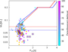 |
Fig. 5 Donor mass as a function of orbital period for 175 systems in our literature catalog with available values for both orbital period and donor mass. The two Knigge et al. (2011) CV evolution tracks from Fig. 1 are shown as reference. See Sect. 4.2 for explanation of markers and color scale, as well as the justification of the selection cut lines. |
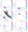 |
Fig. 6 Parameters used in the scorecard to rate the likelihood of a system of being a period-bouncer. See Sect. 4.2 for explanation of markers and color scale, as well as the justification of the selection cut lines. Panel a: WD effective temperature as a function of orbital period for 80 systems in our literature catalog with available information. Panel b: Gaia variability as a function of orbital period for 159 systems in our literature catalog with available information. Panel c: Gaia color –magnitude diagram showing the position of the 145 systems in our literature catalog with available information. The Gaia-DR3 sources with Bailer-Jones et al. (2021) distances and a parallax error of less than 1% of the parallax value are shown in gray as a reference. Panel d: SDSS color –color diagram showing the position of the 83 systems in our literature catalog with available information. Panel e: FUV-NUV color as a function of orbital period for 91 systems in our literature catalog with available information. Panel f: IR color –color diagram showing the position of the 45 systems in our literature catalog with available information. |
5 eROSITA data
To this day, eROSITA has carried out four full-sky surveys, named eRASS 1 to eRASS 4. Source catalogs from eRASS data are produced at Max Planck Institut für extraterrestrische Physik (MPE) in Garching, Germany, with the eROSITA Science Analysis Software System (eSASS) described by Brunner et al. (2022). These catalogs comprise all eRASS sources in the western half of the sky in terms of Galactic coordinates (Galactic longitude l ≥ 180∘), which is the sky area with German data rights. Out of the 192 sources in the literature catalog 80 are located in the German eROSITA sky, eight of which are confirmed period-bouncers listed in Table 1.
5.1 X-ray parameters for the literature sample
To obtain the highest sensitivity for detecting the presumably faint sources from our literature catalog, we used the merged catalog eRASS:3 which was generated from summing data from the first three all-sky surveys. The latest version of the eRASS:3 catalog available to us in December 2023 was produced with the data processing version 0204. Source detection was performed in this catalog for a single eROSITA energy band, 0.2 –2.3 keV.
We choose to work with this eRASS:3 catalog as this was the version used to compile a catalog of CV candidates, which we use as a point of comparison with our work. This catalog of CV candidates (Schwope et al., in prep.) was produced from matching eRASS:3 and Gaia sources using NWAY, a software for probabilistic cross-matching of catalogs (Salvato et al. 2018). It makes use of a Bayesian prior. This was trained on a set of 624 known CVs with well-known X-ray and optical properties. The optical properties used in characterizing the sample are brightness, color, coordinates, parallax, proper motion, and variability. The X-ray properties used are position and flux, and thus implicitly the optical to X-ray flux ratio. The NWAY match applied to eRASS:3 using the CV prior revealed 11 113 candidates with a CV probability >50%, which are used in this paper for comparison to the period-bouncer sample. Full details on the construction of the eRASS:3 sample of CV candidates will be given by Schwope et al. (in prep.).
We corrected the coordinates of the period-bounce candidates in the literature catalog to the mean observing date of eRASS:3 using their Gaia-DR3 proper motions. We then matched them with the eRASS:3 catalog, allowing for a maximum separation of 30″ and enforcing for the separation between optical and X-ray coordinates the condition sepox<3 × RADEC_ERR, where RADEC_ERR is the positional error of the X-ray coordinates in units of arcseconds. This way we found that 51 of the 80 period-bounce candidates from the literature catalog that are in the German eROSITA sky are detected in the eRASS:3 catalog.
This process was performed allowing for all possible matches within 30″. However, each of the 51 detected period-bounce candidates had only one eRASS:3 match within that radius. We then carried out a visual inspection using ESAsky5 30″radius region around the X-ray source to assure that there were no other potential optical counterparts. Out of the 51 period-bounce candidates detected in the eRASS:3 catalog, 45 have no other optical source closer to the eRASS X-ray position than our target and can therefore be confidently categorized as a correct match. Two additional eRASS:3 detections were confirmed as the correct match thanks to previous X-ray detections (XMM-Newton and Chandra) clearly associated with our targets. Out of the remaining four eRASS:3 detections, for one of them the visual inspection revealed an eRASS source at a sepox that is larger than the maximum of 3 × RADEC_ERR that we allowed in the automatic match. For the last three there is another object closer to the eRASS source than our target, such that the X-ray source could not be securely associated with the period-bounce candidate. We present in Table A.1 the 51 sources with an eROSITA detection, where we do not report X-ray parameters for the four sources without a reliable association. These four sources are not considered in the following analysis.
We note in passing that of the 47 systems with safe eRASS:3 detection 31 are detected when using exclusively the first all-sky survey catalog eRASS 16. The use of the combined catalog from three surveys, thus, constitutes a significant improvement, which is not unexpected as our targets are faint and substantially benefit from deeper X-ray exposure.
We proceeded with our analysis for the 47 systems with safe eRASS:3 detection, referred to as “eROSITA subsample“, which includes all eight confirmed period-bouncers located in the German eROSITA sky. In Table A.1 we present their X-ray parameters from eROSITA. In Cols.2 –5, we present the separation sepox, the detection likelihood value (the eRASS:3 catalog has a minimum detection likelihood of 5.0), the number of net source counts, and the count rate. The latter two refer to the 0.2 –2.3 keV band used in eRASS:3. The catalogue uses a power-law model in order to obtain the flux from the count rate. This is not suitable for CVs which are characterized by a thermal plasma. Therefore, we converted the catalog flux from a power-law model to an APEC model using a conversion factor of 1.04 (see Muñoz-Giraldo et al. 2023 for a more detailed description). Using the APEC flux (Col. 6 of Table A.1) together with the Gaia DR3 distances given by Bailer-Jones et al. (2021) we obtained the X-ray luminosity, which was converted into bolometric X-ray luminosity (Lx,bol) in the band 0.1 –12 keV (given in Col. 7) by multiplication with a factor of 1.6 (Muñoz-Giraldo et al. 2023). We then calculated the mass accretion rate for each system taking into consideration if it has a reported value for the WD mass (see Table B.2). For those systems with a reported WD mass we used this value together with the WD radius obtained with the Nauenberg (1972) mass-radius relation. For the systems without a WD mass we used 0.8 M⊙, which is the mean mass of WDs in CVs (Pala et al. 2022), and the corresponding radius of 7 × 108 cm from the Nauenberg (1972) mass-radius relation. Only one system, TCP 1537, does not have a reported Gaia DR3 distance, which prevents us from calculating an X-ray luminosity and mass accretion rate for this period-bounce candidate.
5.2 X-ray parameter space of period-bouncers
Using the final scores assigned to the confirmed period-bouncers (see Table 3) together with the X-ray results from eROSITA (see Table A.1) we can establish two new parameters, X-ray-to-optical flux ratio (Fx/Fopt) and bolometric X-ray luminosity, that will aid in the future identification of highly likely period-bounce candidates from eROSITA data. A possible third new parameter, the mass accretion rate (Ṁacc), could be used for cases with known WD mass, considering that using the mean WD mass and radius gives a distribution indistinguishable from the one obtained using the X-ray luminosity. As less than half of the period-bounce candidates with eROSITA data have an individually determined WD mass, Ṁacc would not yield additional information on the sample and we do not use it to define selection cuts for period-bouncers.
In Figs. 7 and 8, we have placed the eROSITA subsample in two diagrams combining X-ray and optical data. We compare the position of this sample with the overall catalog of eROSITA selected CV candidates (Schwope et al., in prep) introduced in Sect. 5.1. The eROSITA detected confirmed period-bouncers from Table 1 are highlighted using black boxes.
Figure 7 presents the X-ray-to-optical flux ratio versus Gaia color, where the majority of both the overall eROSITA CV candidate population and our eROSITA subsample display -1 ≲ log(Fx/Fopt) ≲ 0. This is to be expected in systems with low mass transfer rate including different CV types such as dwarf novae, polars and intermediate polars, which make up the bulk of the observed CV population. Even though this parameter is not meant to be used on its own to determine new period-bounce candidates, it serves as an important check that the system does not display very small values of X-ray-to-optical flux ratio, that would indicate a system with a very high mass transfer rate (e.g., nova-like variables) and thus disqualify the system from being a period-bouncer.
Figure 8 shows the bolometric X-ray luminosity versus Gaia color, where we identify a region preferably dominated by highly likely period-bouncers. In this diagram, the highly likely period-bouncers from the eROSITA subsample are considerably differentiated from the overall eROSITA CV candidate population displaying a lower bolometric X-ray luminosity of Lx,bol ≈ 1030 erg s−1. Together with their relatively blue Gaia color Lx, bol proves to be a powerful tool for identifying new period-bounce candidates from eROSITA data, as, compared to most other CV candidates, probable period-bouncers present both bluer colors (because they are WD dominated) and lower X-ray luminosities (because of their low mass accretion rate). Applying selection cuts based on the upper limits for the X-ray luminosity (log(Lx,bol)≤ 30.4 [erg s−1]) and Gaia color (GBP-GRP≤ 0.35) exhibited by systems from our catalog that have already been confirmed as being period-bouncers (see lower left rectangle in Fig. 8) separates 971 CV candidates from the rest of the overall eROSITA CV candidate population. Additionally, we checked that they are low mass transfer rate systems using the X-ray-to-optical flux ratio (-1.21 ≤ log(Fx/Fopt)≤ 0) exhibited by the confirmed period-bouncers in our catalog, finding that 775 of them fulfill both X-ray criteria defined for confirmed period-bouncers from eROSITA.
We show in Fig. 9 the relationship between X-ray luminosity and distance. The red line gives the lower limit for the eRASS:3 luminosity calculated for the limiting X-ray flux of 2 × 10⁻¹⁴ erg cm−2 (Muñoz-Giraldo et al. 2023). Two things are immediately apparent from Fig. 9. First, at a given luminosity period-bounce candidates tend to have smaller distances than the majority of CV candidates. This is expected as period-bouncers are intrinsically faint. Secondly, for a given distance, our period-bounce candidates are among the sources with the highest X-ray luminosity, probably due to (non-X-ray) selection effects of the literature catalogs they were pulled from. This means that there might be a significant population of period-bouncers at short distances with X-ray luminosities lower than the period-bounce candidates identified in this work but higher than the eRASS:3 limit. These systems have yet to be singled out and studied.
In order to select this missing population of period-bouncers in eROSITA data we should look into the 775 selected CV candidates that are systems with low mass transfer rates as well as fulfill the selection cuts shown in Fig. 8. These systems are shown as grey dots in Fig. 9 located fairly close to the luminosity limit in eRASS:3 for period-bouncers (see red line in Fig. 9).
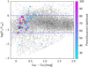 |
Fig. 7 X-ray-to-optical flux ratio as a function of Gaia colors showing the position of the 46 systems in our literature catalog found in eRASS:3. We show in grey as reference a population of CV candidates found in eRASS:3. |
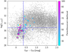 |
Fig. 8 Bolometric X-ray luminosity as a function of Gaia colors showing the position of the 46 systems in our literature catalog found in eRASS:3. We show in grey as reference a population of CV candidates found in eRASS:3. See text for the justification of the selection cut lines. |
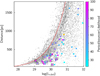 |
Fig. 9 Distance from Bailer-Jones et al. (2021) versus bolometric X-ray luminosity showing the position of the 46 systems in our literature catalog detected in eRASS:3 with respect to the average eRASS:3 sensitivity limit marked by the red line. We show in black the population of CV candidates found in eRASS:3, and in grey a subsample of 775 CV candidates of them that we have selected as period-bounce candidates. |
6 Conclusions
One of our main goals in this work has been to establish the X-ray properties of the class of period-bounce CVs, specifically using new data from the eROSITA all-sky surveys. We explored the eRASS:3 catalog with a sample of 17 confirmed period-bouncers and 175 additional candidates that we compiled from the literature. We established two selection cuts based on the X-ray-to-optical flux ratio and the X-ray luminosity observed from the already confirmed period-bouncers. We found seven candidates with high likelihood of being a period-bounce system according to our multiparameter scorecard within these X-ray selection cuts (see Cols. 10 –12 in Table A.1). This means that they appear very similar to known period-bouncers in our multiwavelength study including X-rays. On this basis, we can confidently suggest seven systems in our literature catalog as new period-bouncers. Four of these seven systems (LP 731-60, EG Cnc, SDSS J12160+0520, and HV Vir) had already been suggested as potential period-bouncers, however, a confident classification was not evident to us from the literature. The remaining three systems (1RXS J02323-3718, PM J12192+2049, and CRTS J10441+2113) were only mentioned in the literature as WZ Sge-type objects. None of the new period-bouncers have a detected late-type donor mainly due to the lack of in-depth studies of these sources. Future detailed spectroscopic studies will shed more light on their status as period-bouncers.
This new addition of confirmed period-bouncers represents an increase in the population of some 40%, bringing the number of this elusive class of CVs to 24 and establishing eROSITA as a powerful tool for the characterization and identification of period-bouncers. However, despite this substantial increase of the known population of period-bounce CVs, it still remains well below the numbers expected by theoretical models. We foresee that a further exploitation of eROSITA data might boost the population number to the predicted levels, especially considering that the X-ray faint period-bounce population has yet to be adequately discovered.
In an exploratory study, we tentatively identified a 500 pc volume-limited sample of potential period-bouncers from the overall CV population presented in a new eROSITA-selected catalog (Schwope et al., in prep.). The 500 pc boundary is motivated by the limitation on the accuracy of distance measurements that can be achieved with Gaia for faint objects (see Fig. 4) and the eRASS sensitivity limit (Fig. 9).
First, in our catalog of period-bounce candidates, 77 of the 81 systems within 500 pc have a fractional distance error smaller than 20, including all 17 confirmed period-bouncers from Table 1 and all 7 new eROSITA-confirmed period-bouncers. Secondly, when we take the mean X-ray luminosity of the 8 confirmed period bouncers detected in eRASS:3 (log(Lx,bol) = 29.74 [erg s−1]) as a typical X-ray luminosity for this class of objects the average eRASS:3 flux limit yields a distance limit of 480 pc. Thus, a rough distance limit of 500 pc seems appropriate for a meaningful period-bouncer population study.
Within 500 pc, the population of CV candidates from eRASS:3 is made up of 1770 systems, of which 543 have been selected as potential period-bounce candidates using our eROSITA X-ray selection cuts, representing 31% of the overall CV candidate population. Even though this result would only place the population of period-bouncers towards the lower end of the expected by evolutionary CV models (40% to 80%), it would be an encouraging indicator that more period-bouncers have not been discovered mainly due to observational constrains rather than overestimation from CV evolution models.
In the near future, we will seek to systematically uncover the 500 pc sample of period-bouncers. We aim to carry out an in-depth study of the 81 candidates from the catalog presented in this work and the 543 new eROSITA CV candidates we selected as potential period-bouncers using the X-ray selection cuts.
The confirmation or rejection of the systems from this sample will provide a benchmark for population studies of CVs around the period-bounce region.
Acknowledgements
We thank an anonymous referee for reviewing the original manuscript and giving helpful comments and useful advice. Daniela Muñoz-Giraldo acknowledges financial support from Deutsche Forschungsgemeinschaft (DFG) under grant number STE 1068/6-1. This work is based on data from eROSITA, the primary instrument aboard SRG, a joint Russian-German science mission supported by the Russian Space Agency (Roskosmos), in the interests of the Russian Academy of Sciences represented by its Space Research Institute (IKI), and the Deutsches Zentrum für Luft- und Raumfahrt (DLR). The SRG spacecraft was built by Lavochkin Association (NPOL) and its subcontractors, and is operated by NPOL with support from the Max Planck Institute for Extraterrestrial Physics (MPE). The development and construction of the eROSITA X-ray instrument was led by MPE, with contributions from the Dr. Karl Remeis Observatory Bamberg and ECAP (FAU Erlangen-Nürnberg), the University of Hamburg Observatory, the Leibniz Institute for Astrophysics Potsdam (AIP), and the Institute for Astronomy and Astrophysics of the University of Tübingen, with the support of DLR and the Max Planck Society. The Argelander Institute for Astronomy of the University of Bonn and the Ludwig Maximilians Universität München also participated in the science preparation for ero. The eROSITA data shown here were processed using the eSASS/NRTA software system developed by the German eROSITA consortium. This work has made use of data from the European Space Agency (ESA) mission Gaia (https://www.cosmos.esa.int/gaia), processed by the Gaia Data Processing and Analysis Consortium (DPAC, https://www.cosmos.esa.int/web/gaia/dpac/consortium). Funding for the DPAC has been provided by national institutions, in particular the institutions participating in the Gaia Multilateral Agreement. This publication makes use of VOSA, developed under the Spanish Virtual Observatory (https://svo.cab.inta-csic.es) project funded by MCIN/AEI/10.13039/501100011033/ through grant PID2020-112949GB-I00. VOSA has been partially updated by using funding from the European Union’s Horizon 2020 Research and Innovation Programme, under Grant Agreement n∘ 776403 (EXOPLANETS-A).
Appendix A X-ray parameters for eROSITA detected systems
Table A.1 gives the X-ray parameters from the eROSITA merged catalog eRASS:3 for the detected sources from the literature catalog, known as the eROSITA subsample, including the distance used to calculate the X-ray luminosity and the final period-bouncer score. Values are given for the eROSITA single band (0.2-2.3 keV).
Appendix B Abridged literature catalog table
Table B.1 gives a brief description of the columns available in the complete version of our literature catalog. Selected columns showing system parameters from the literature are given in Table B.2.
Content of the 66 columns in our literature catalog of period-bounce candidates, corresponding to values obtained from the literature and from photometry.
Shortened version of our period-bounce candidates catalog showing relevant properties of the systems.
Appendix C Examples for SED types
We define 3 typical cases for SEDs of pre-bounce CVs, CVs at the period minimum and post-bounce CVs with the following criteria: excess setting in at wavelengths shorter than 12483 Å (J-band) for CVs before the period-bounce, excess setting in at wavelengths between 12483Å and 22010Å (K-band) for CVs around the period-bounce, and excess setting in at wavelengths longer than 22010 for CVs significantly after the period-bounce.
To determine the onset wavelength of the excess in the SED we used VOSA, where we fitted a WD model (Koester 2010) to the SED of each period-bounce candidate in our literature catalog initially giving as input a range of ±1000 K around the WD temperature found in the literature. When necessary, we adjusted the temperature range to obtain a better fit specifically for the GALEX points considering that it is in the UV bands where we get the best constraints on the WD. The final WD temperature and log(g) values used in the fit are reported in the top part of each figure. We did not consider extinction. VOSA suggests a point for the beginning of the excess (vertical dashed line in Figs. C.1, C.2, C.3 and C.4) which, in most cases, we used to assign the corresponding points in our scorecard. There were a few cases (see Fig. C.4) where it was clear that the excess starts at a shorter wavelength, in which case we selected ourselves the shorter band as the point of beginning of the excess.
We use 4 different systems from our catalog to illustrate different SED cases. V379 Vir (Fig. C.1), with an excess starting at the K-band, is a confirmed magnetic period-bouncer with a spectroscopically detected L8 donor (Farihi et al. 2008). V406 Vir (Fig. C.2), with an excess starting at the K-band, is a confirmed non-magnetic period-bouncer with a spectroscopically detected L3 donor (Pala et al. 2019). CRTS J122221.6-311525 (Fig. C.3), with an excess starting at the WISE1-band, is a confirmed non-magnetic period-bouncer with a photometrically detected L0 donor (Neustroev et al. 2017). EF Eri is an already confirmed pre-bounce magnetic system with an excess starting in the J-band (Fig. C.4).
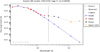 |
Fig. C.1 WD fit to the SED of V379 Vir. VOSA marks the excess starting at K-band. |
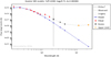 |
Fig. C.2 WD fit to the SED of V406 Vir. VOSA marks the excess starting at K-band. |
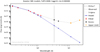 |
Fig. C.3 WD fit to the SED of CRTS J122221.6-311525. VOSA marks the excess starting at WISE 1 band. |
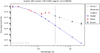 |
Fig. C.4 WD fit to the SED of EF Eri. VOSA marks the excess starting at WISE 1 band, but it is clear to us that it starts at J-band. |
Magnetic systems, like V379 Vir and EF Eri, are expected to present cyclotron humps (Wickramasinghe 1988). From comparing Figs C.1 and C.2, a clear increased emission between 21000Å and 46000Åcan be observed in the SED of V379 Vir most likely due to cyclotron humps. However, even when considering this additional feature, the IR excess in V379 Vir still starts at the K-band as expected for period-bouncers. EF Eri, a known magnetic pre-bounce systems, also presents cyclotron humps in the SED but associated with shorter wavelengths that lead to IR excess starting at J-band, marking the system as not a period-bouncer.
References
- Ahumada, R., Allende Prieto, C., Almeida, A., et al. 2022, VizieR On line Data Catalog: V/154 [Google Scholar]
- Amantayeva, A., Zharikov, S., Page, K., et al. 2021, ApJ, 918, 58 [NASA ADS] [CrossRef] [Google Scholar]
- Araujo-Betancor, S., Gänsicke, B., Hagen, H.-J., et al. 2005, A&A, 430, 629 [NASA ADS] [CrossRef] [EDP Sciences] [Google Scholar]
- Audard, M., Osten, R., Brown, A., et al. 2007, A&A, 471, L63 [NASA ADS] [CrossRef] [EDP Sciences] [Google Scholar]
- Bailer-Jones, C. A. 2015, PASP, 127, 994 [NASA ADS] [CrossRef] [Google Scholar]
- Bailer-Jones, C. A. L., Rybizki, J., Fouesneau, M., Demleitner, M., & Andrae, R. 2021, AJ, 161, 147 [Google Scholar]
- Bayo, A., Rodrigo, C., Barrado Y Navascués, D., et al. 2008, A&A, 492, 277 [NASA ADS] [CrossRef] [EDP Sciences] [Google Scholar]
- Belloni, D., Schreiber, M. R., Pala, A. F., et al. 2020, MNRAS, 491, 5717 [Google Scholar]
- Beuermann, K., Burwitz, V., Reinsch, K., Schwope, A., & Thomas, H.-C. 2021, A&A, 645, A56 [NASA ADS] [CrossRef] [EDP Sciences] [Google Scholar]
- Bianchi, L., Shiao, B., & Thilker, D. 2017, ApJS, 230, 24 [Google Scholar]
- Breedt, E., Gaensicke, B. T., Girven, J., et al. 2012, MNRAS, 423, 1437 [NASA ADS] [CrossRef] [Google Scholar]
- Brunner, H., Liu, T., Lamer, G., et al. 2022, A&A, 661, A1 [NASA ADS] [CrossRef] [EDP Sciences] [Google Scholar]
- Burleigh, M. R., Marsh, T., Gänsicke, B., et al. 2006, MNRAS, 373, 1416 [NASA ADS] [CrossRef] [Google Scholar]
- Cropper, M. 1990, Space Sci. Rev., 54, 195 [CrossRef] [Google Scholar]
- Cutri, R. M., Wright, E. L., Conrow, T., et al. 2021, VizieR Online Data Catalog: II/328 [Google Scholar]
- De Luca, A., Stelzer, B., Burgasser, A. J., et al. 2020, A&A, 634, A13 [NASA ADS] [CrossRef] [EDP Sciences] [Google Scholar]
- Echevarría, J., Zharikov, S., & Mora Zamora, I. 2023, MNRAS, 526, 5110 [CrossRef] [Google Scholar]
- Farihi, J., Burleigh, M., & Hoard, D. 2008, ApJ, 674, 421 [NASA ADS] [CrossRef] [Google Scholar]
- Gaia Collaboration 2022, VizieR Online Data Catalog: I/355 [Google Scholar]
- Gänsicke, B., Dillon, M., Southworth, J., et al. 2009, MNRAS, 397, 2170 [CrossRef] [Google Scholar]
- Gentile Fusillo, N., Tremblay, P., Cukanovaite, E., et al. 2021, MNRAS, 508, 3877 [NASA ADS] [CrossRef] [Google Scholar]
- Girven, J., Gänsicke, B., Steeghs, D., & Koester, D. 2011, MNRAS, 417, 1210 [NASA ADS] [CrossRef] [Google Scholar]
- Goliasch, J., & Nelson, L. 2015, ApJ, 809, 80 [Google Scholar]
- Guidry, J. A., Vanderbosch, Z. P., Hermes, J., et al. 2021, ApJ, 912, 125 [NASA ADS] [CrossRef] [Google Scholar]
- Harrison, T. E. 2015, ApJ, 816, 4 [Google Scholar]
- Howell, S. B., Nelson, L. A., & Rappaport, S. 2001, ApJ, 550, 897 [Google Scholar]
- Howell, S. B., Walter, F. M., Harrison, T. E., et al. 2006, ApJ, 652, 709 [NASA ADS] [CrossRef] [Google Scholar]
- Inight, K., Gänsicke, B. T., Breedt, E., et al. 2021, MNRAS, 504, 2420 [NASA ADS] [CrossRef] [Google Scholar]
- Inight, K., Gänsicke, B. T., Breedt, E., et al. 2023a, MNRAS, 524, 4867 [NASA ADS] [CrossRef] [Google Scholar]
- Inight, K., Gänsicke, B. T., Schwope, A., et al. 2023b, MNRAS, 525, 3597 [NASA ADS] [CrossRef] [Google Scholar]
- Ishioka, R., Sekiguchi, K., & Maehara, H. 2007, PASJ, 59, 929 [NASA ADS] [CrossRef] [Google Scholar]
- Jiménez-Esteban, F., Torres, S., Rebassa-Mansergas, A., et al. 2018, MNRAS, 480, 4505 [CrossRef] [Google Scholar]
- Kato, T. 2015, PASJ, 67, 108 [NASA ADS] [CrossRef] [Google Scholar]
- Kato, T. 2022, arXiv e-prints [arXiv:2201.02945] [Google Scholar]
- Kato, T., & Osaki, Y. 2013, PASJ, 65, 115 [NASA ADS] [CrossRef] [Google Scholar]
- Kato, T., Imada, A., Uemura, M., et al. 2009, PASJ, 61, S395 [NASA ADS] [Google Scholar]
- Kawka, A., Vennes, S., Ferrario, L., et al. 2021, MNRAS, 507, L30 [NASA ADS] [CrossRef] [Google Scholar]
- Kimura, M., Isogai, K., Kato, T., et al. 2018, PASJ, 70, 47 [NASA ADS] [CrossRef] [Google Scholar]
- King, A. 1988, Q. J. Roy. Astron. Soc., 29, 1 [NASA ADS] [Google Scholar]
- Kirkpatrick, J. D., & McCarthy Jr, D. W. 1994, AJ, 107, 333 [NASA ADS] [CrossRef] [Google Scholar]
- Knigge, C. 2006, MNRAS, 373, 484 [NASA ADS] [CrossRef] [Google Scholar]
- Knigge, C., Baraffe, I., & Patterson, J. 2011, ApJS, 194, 28 [Google Scholar]
- Koester, D. 2010, Mem. Soc. Astron. Italiana, 81, 921 [NASA ADS] [Google Scholar]
- Kolb, U. 1993, A&A, 271, 149 [NASA ADS] [Google Scholar]
- Kolb, U., & Baraffe, I. 1999, MNRAS, 309, 1034 [NASA ADS] [CrossRef] [Google Scholar]
- Kolb, U., King, A., & Ritter, H. 1998, MNRAS, 298, L29 [NASA ADS] [CrossRef] [Google Scholar]
- Kruckow, M. U., Neunteufel, P. G., Di Stefano, R., Gao, Y., & Kobayashi, C. 2021, ApJ, 920, 86 [NASA ADS] [CrossRef] [Google Scholar]
- Lawrence, A., Warren, S., Almaini, O., et al. 2007, MNRAS, 379, 1599 [NASA ADS] [CrossRef] [Google Scholar]
- Lindegren, L., Klioner, S., Hernández, J., et al. 2021, A&A, 649, A2 [NASA ADS] [CrossRef] [EDP Sciences] [Google Scholar]
- Littlefair, S., Dhillon, V., & Martin, E. 2003, MNRAS, 340, 264 [NASA ADS] [CrossRef] [Google Scholar]
- Littlefair, S., Dhillon, V., Marsh, T., et al. 2008, MNRAS, 388, 1582 [NASA ADS] [CrossRef] [Google Scholar]
- Liu, Y., Hwang, H.-C., Zakamska, N. L., & Thorstensen, J. R. 2023, MNRAS, 522, 2719 [NASA ADS] [CrossRef] [Google Scholar]
- Longstaff, E., Casewell, S., Wynn, G., et al. 2019, MNRAS, 484, 2566 [NASA ADS] [CrossRef] [Google Scholar]
- Luri, X., Brown, A., Sarro, L., et al. 2018, A&A, 616, A9 [NASA ADS] [CrossRef] [EDP Sciences] [Google Scholar]
- McAllister, M., Littlefair, S., Dhillon, V., et al. 2017, MNRAS, 467, 1024 [NASA ADS] [CrossRef] [Google Scholar]
- McAllister, M., Littlefair, S., Parsons, S., et al. 2019, MNRAS, 486, 5535 [NASA ADS] [CrossRef] [Google Scholar]
- McMahon, R. G., Banerji, M., Gonzalez, E., et al. 2021, VizieR Online Data Catalog: II/367 [Google Scholar]
- Mestel, L. 1968, MNRAS, 138, 359 [NASA ADS] [CrossRef] [Google Scholar]
- Meyer, F., & Meyer-Hofmeister, E. 1984, A&A, 132, 143 [NASA ADS] [Google Scholar]
- Muñoz-Giraldo, D., Stelzer, B., de Martino, D., & Schwope, A. 2023, A&A, 676, A7 [NASA ADS] [CrossRef] [EDP Sciences] [Google Scholar]
- Nauenberg, M. 1972, ApJ, 175, 417 [NASA ADS] [CrossRef] [Google Scholar]
- Neustroev, V. V., & Mäntynen, I. 2023, MNRAS, 523, 6114 [NASA ADS] [CrossRef] [Google Scholar]
- Neustroev, V., Marsh, T. R., Zharikov, S., et al. 2017, MNRAS, 467, 597 [NASA ADS] [Google Scholar]
- Osaki, Y. 1989, PASJ, 41, 1005 [NASA ADS] [Google Scholar]
- Otulakowska-Hypka, M., Olech, A., & Patterson, J. 2016, MNRAS, 460, 2526 [CrossRef] [Google Scholar]
- Owens, D., Xu, S., Manjavacas, E., et al. 2023, AJ, 166, 5 [NASA ADS] [CrossRef] [Google Scholar]
- Paczynski, B. 1976, in IAU Symp., 73 (Cambridge University Press), 75 [NASA ADS] [Google Scholar]
- Paczynski, B., & Sienkiewicz, R. 1983, ApJ, 268, 825 [NASA ADS] [CrossRef] [Google Scholar]
- Pala, A. F., Gänsicke, B., Townsley, D., et al. 2017, MNRAS, 466, 2855 [NASA ADS] [CrossRef] [Google Scholar]
- Pala, A. F., Schmidtobreick, L., Tappert, C., Gänsicke, B. T., & Mehner, A. 2018, MNRAS, 481, 2523 [NASA ADS] [CrossRef] [Google Scholar]
- Pala, A. F., Gänsicke, B. T., Marsh, T., et al. 2019, MNRAS, 483, 1080 [NASA ADS] [CrossRef] [Google Scholar]
- Pala, A., Gänsicke, B., Breedt, E., et al. 2020, MNRAS, 494, 3799 [NASA ADS] [CrossRef] [Google Scholar]
- Pala, A., Gänsicke, B., Belloni, D., et al. 2022, MNRAS, 510, 6110 [NASA ADS] [CrossRef] [Google Scholar]
- Patterson, J. 1994, PASP, 106, 209 [Google Scholar]
- Patterson, J. 1998, PASP, 110, 1132 [CrossRef] [Google Scholar]
- Patterson, J. 2011, MNRAS, 411, 2695 [NASA ADS] [CrossRef] [Google Scholar]
- Patterson, J., Masi, G., Richmond, M. W., et al. 2002, PASP, 114, 721 [NASA ADS] [CrossRef] [Google Scholar]
- Patterson, J., Kemp, J., Harvey, D. A., et al. 2005a, PASP, 117, 1204 [Google Scholar]
- Patterson, J., Thorstensen, J. R., & Kemp, J. 2005b, PASP, 117, 427 [NASA ADS] [CrossRef] [Google Scholar]
- Politano, M. 1996, ApJ, 465, 338 [NASA ADS] [CrossRef] [Google Scholar]
- Predehl, P., Andritschke, R., Arefiev, V., et al. 2021, A&A, 647, A1 [EDP Sciences] [Google Scholar]
- Pretorius, M. L., Knigge, C., & Schwope, A. D. 2013, MNRAS, 432, 570 [Google Scholar]
- Rappaport, S., Joss, P. C., & Webbink, R. F. 1982, ApJ, 254, 616 [NASA ADS] [CrossRef] [Google Scholar]
- Ritter, H. 1991, in High Energy Astrophysics: Compact Stars and Active Galaxies (Proc. 3rd Chinese Academy of Sciences and Max-Planck-Society Workshop, Huangshan, China, 1990), ed. Q.B. Li (Singapore: World Scientific), 107 [Google Scholar]
- Salvato, M., Buchner, J., Budavári, T., et al. 2018, MNRAS, 473, 4937 [Google Scholar]
- Santisteban, J. V. H., Knigge, C., Littlefair, S. P., et al. 2016, Nature, 533, 366 [NASA ADS] [CrossRef] [Google Scholar]
- Santisteban, J. H., Knigge, C., Pretorius, M., Sullivan, M., & Warner, B. 2018, MNRAS, 473, 3241 [NASA ADS] [CrossRef] [Google Scholar]
- Savoury, C., Littlefair, S., Dhillon, V., et al. 2011, MNRAS, 415, 2025 [NASA ADS] [CrossRef] [Google Scholar]
- Savoury, C., Littlefair, S. P., Marsh, T. R., et al. 2012, MNRAS, 422, 469 [NASA ADS] [CrossRef] [Google Scholar]
- Schmidt, G. D., Szkody, P., Silvestri, N. M., et al. 2005, ApJ, 630, L173 [NASA ADS] [CrossRef] [Google Scholar]
- Schreiber, M., Zorotovic, M., & Wijnen, T. 2016, MNRAS, 455, L16 [NASA ADS] [CrossRef] [Google Scholar]
- Schreiber, M. R., Belloni, D., Gänsicke, B. T., Parsons, S. G., & Zorotovic, M. 2021, Nat. Astron., 5, 648 [NASA ADS] [CrossRef] [Google Scholar]
- Schreiber, M. R., Belloni, D., & van Roestel, J. 2023, A&A, 679, A8 [NASA ADS] [CrossRef] [EDP Sciences] [Google Scholar]
- Schwope, A., & Christensen, L. 2010, A&A, 514, A89 [NASA ADS] [CrossRef] [EDP Sciences] [Google Scholar]
- Schwope, A., Worpel, H., & Traulsen, I. 2021, A&A, 646, A181 [NASA ADS] [CrossRef] [EDP Sciences] [Google Scholar]
- Skrutskie, M., Cutri, R., Stiening, R., et al. 2006, AJ, 131, 1163 [Google Scholar]
- Southworth, J., Gänsicke, B., Marsh, T., et al. 2006, MNRAS, 373, 687 [NASA ADS] [CrossRef] [Google Scholar]
- Spruit, H. C., & Ritter, H. 1983, A&A, 124, 267 [NASA ADS] [Google Scholar]
- Stelzer, B., de Martino, D., Casewell, S., Wynn, G., & Roy, M. 2017, A&A, 598, L6 [NASA ADS] [CrossRef] [EDP Sciences] [Google Scholar]
- Sunyaev, R., Arefiev, V., Babyshkin, V., et al. 2021, A&A, 656, A132 [NASA ADS] [CrossRef] [EDP Sciences] [Google Scholar]
- Taylor, M. B. 2005, in Astronomical Data Analysis Software and Systems XIV, 347, 29 [NASA ADS] [Google Scholar]
- Unda-Sanzana, E., Marsh, T., Gänsicke, B. T., et al. 2008, MNRAS, 388, 889 [NASA ADS] [CrossRef] [Google Scholar]
- Uemura, M., Kato, T., Nogami, D., & Ohsugi, T. 2010, PASJ, 62, 613 [NASA ADS] [Google Scholar]
- Verbunt, F., & Zwaan, C. 1981, A&A, 100, L7 [NASA ADS] [Google Scholar]
- Vogt, N. 1980, A&A, 88, 66 [NASA ADS] [Google Scholar]
- Warner, B. 1995, Cataclysmic Variable Stars, 28 (Cambridge University Press) [CrossRef] [Google Scholar]
- Webbink, R., & Wickramasinghe, D. 2002, MNRAS, 335, 1 [NASA ADS] [CrossRef] [Google Scholar]
- Whitehurst, R. 1988, MNRAS, 232, 35 [NASA ADS] [Google Scholar]
- Wickramasinghe, D. T. 1988, in Polarized Radiation of Circumstellar Origin, eds. G. V. Coyne, A. M. Magalhaes, A. F. Moffat, R. E. Schulte-Ladbeck, & S. Tapia, 199 [Google Scholar]
- Wickramasinghe, D., & Ferrario, L. 2000, PASP, 112, 873 [NASA ADS] [CrossRef] [Google Scholar]
- Wijnen, T., Zorotovic, M., & Schreiber, M. 2015, A&A, 577, A143 [NASA ADS] [CrossRef] [EDP Sciences] [Google Scholar]
- Wild, J., Littlefair, S., Ashley, R., et al. 2022, MNRAS, 509, 5086 [Google Scholar]
- Zharikov, S., Tovmassian, G., Aviles, A., et al. 2013, A&A, 549, A77 [NASA ADS] [CrossRef] [EDP Sciences] [Google Scholar]
- Zorotovic, M., Schreiber, M. R., & Gänsicke, B. 2011, A&A, 536, A42 [NASA ADS] [CrossRef] [EDP Sciences] [Google Scholar]
SIMBAD stands for Set of Identifications, Measurements and Bibliography for Astronomical Data, available at http://simbad.cds.unistra.fr/simbad
The source catalog used in our work is all_s3_SourceCat1B_221007_poscorr_mpe_clean.fits (for eRASS:3).
The source catalog used in our work is the 020 version of all_e1_SourceCat3B_221031_poscorr_mpe_clean.fits (for eRASS1).
All Tables
Content of the 66 columns in our literature catalog of period-bounce candidates, corresponding to values obtained from the literature and from photometry.
Shortened version of our period-bounce candidates catalog showing relevant properties of the systems.
All Figures
|
Fig. 1 Donor mass as a function of orbital period for the objects in our literature catalog of period-bounce candidates. The color and shape corresponds to the catalogs from which we took the system (and that are listed in the legend). Two CV evolution tracks from Knigge et al. (2011) are shown as reference: the standard track considering angular momentum loss only due to gravitational radiation (blue) and a revised track that considers enhanced angular momentum loss (orange). |
| In the text | |
|
Fig. 2 Evolution for magnetic and non-magnetic CVs for the 94 systems in our literature catalog with information about the magnetism of the WD. Point of period reversal (Mdonor ≈0. 058 M⊙) is shown by the green dashed line. The two Knigge et al. (2011) CV evolution tracks from Fig. 1 are shown as reference. |
| In the text | |
|
Fig. 3 Distribution of the orbital period for 190 systems in our literature catalog with values from the literature. The vertical green line is an estimate of Pspike using a Gaussian fit to the distribution of systems with orbital periods between 77 min and 87 min. |
| In the text | |
|
Fig. 4 Comparison between the distance obtained by Bailer-Jones et al. (2021) and by using the inverse of the parallax. |
| In the text | |
|
Fig. 5 Donor mass as a function of orbital period for 175 systems in our literature catalog with available values for both orbital period and donor mass. The two Knigge et al. (2011) CV evolution tracks from Fig. 1 are shown as reference. See Sect. 4.2 for explanation of markers and color scale, as well as the justification of the selection cut lines. |
| In the text | |
|
Fig. 6 Parameters used in the scorecard to rate the likelihood of a system of being a period-bouncer. See Sect. 4.2 for explanation of markers and color scale, as well as the justification of the selection cut lines. Panel a: WD effective temperature as a function of orbital period for 80 systems in our literature catalog with available information. Panel b: Gaia variability as a function of orbital period for 159 systems in our literature catalog with available information. Panel c: Gaia color –magnitude diagram showing the position of the 145 systems in our literature catalog with available information. The Gaia-DR3 sources with Bailer-Jones et al. (2021) distances and a parallax error of less than 1% of the parallax value are shown in gray as a reference. Panel d: SDSS color –color diagram showing the position of the 83 systems in our literature catalog with available information. Panel e: FUV-NUV color as a function of orbital period for 91 systems in our literature catalog with available information. Panel f: IR color –color diagram showing the position of the 45 systems in our literature catalog with available information. |
| In the text | |
|
Fig. 7 X-ray-to-optical flux ratio as a function of Gaia colors showing the position of the 46 systems in our literature catalog found in eRASS:3. We show in grey as reference a population of CV candidates found in eRASS:3. |
| In the text | |
|
Fig. 8 Bolometric X-ray luminosity as a function of Gaia colors showing the position of the 46 systems in our literature catalog found in eRASS:3. We show in grey as reference a population of CV candidates found in eRASS:3. See text for the justification of the selection cut lines. |
| In the text | |
|
Fig. 9 Distance from Bailer-Jones et al. (2021) versus bolometric X-ray luminosity showing the position of the 46 systems in our literature catalog detected in eRASS:3 with respect to the average eRASS:3 sensitivity limit marked by the red line. We show in black the population of CV candidates found in eRASS:3, and in grey a subsample of 775 CV candidates of them that we have selected as period-bounce candidates. |
| In the text | |
|
Fig. C.1 WD fit to the SED of V379 Vir. VOSA marks the excess starting at K-band. |
| In the text | |
|
Fig. C.2 WD fit to the SED of V406 Vir. VOSA marks the excess starting at K-band. |
| In the text | |
|
Fig. C.3 WD fit to the SED of CRTS J122221.6-311525. VOSA marks the excess starting at WISE 1 band. |
| In the text | |
|
Fig. C.4 WD fit to the SED of EF Eri. VOSA marks the excess starting at WISE 1 band, but it is clear to us that it starts at J-band. |
| In the text | |
Current usage metrics show cumulative count of Article Views (full-text article views including HTML views, PDF and ePub downloads, according to the available data) and Abstracts Views on Vision4Press platform.
Data correspond to usage on the plateform after 2015. The current usage metrics is available 48-96 hours after online publication and is updated daily on week days.
Initial download of the metrics may take a while.