| Issue |
A&A
Volume 687, July 2024
|
|
|---|---|---|
| Article Number | A279 | |
| Number of page(s) | 15 | |
| Section | Galactic structure, stellar clusters and populations | |
| DOI | https://doi.org/10.1051/0004-6361/202449779 | |
| Published online | 18 July 2024 | |
The population of Galactic supernova remnants in the TeV range
1
Universität Potsdam, Institut für Physik und Astronomie, Campus Golm, Haus 28, Karl-Liebknecht-Str. 24/25, 14476 Potsdam-Golm, Germany
e-mail: This email address is being protected from spambots. You need JavaScript enabled to view it.
2
Observatoire de Paris, PSL Research University, 61 Avenue de l’Observatoire, Paris, France
3
Institute of Space Sciences (ICE, CSIC), Campus UAB, Carrer de Can Magrans s/n, 08193 Barcelona, Spain
Received:
28
February
2024
Accepted:
26
April
2024
Abstract
Context. Supernova remnants (SNRs) are likely to be significant sources of cosmic rays up to the knee of the local cosmic-ray (CR) spectrum. They produce gamma rays in the very-high-energy (VHE) (E > 0.1 TeV) range mainly via two mechanisms: hadronic interactions of accelerated protons with the interstellar medium and leptonic interactions of accelerated electrons with soft photons. Observations with current instruments have lead to the detection of about a dozen SNRs emitting VHE gamma rays and future instruments should significantly increase this number. Yet, the details of particle acceleration at SNRs and of the mechanisms producing VHE gamma-rays at SNRs remain poorly understood.
Aims. We aim to study the population of SNRs detected in the TeV range and its properties and confront it to simulated samples in order to address fundamental questions concerning particle acceleration at SNR shocks. Such questions concern the spectrum of accelerated particles, the efficiency of particle acceleration, and the gamma-ray emission being dominated by hadronic or leptonic interactions.
Methods. By means of Monte Carlo methods, we simulated the population of SNRs in the gamma-ray domain and confronted our simulations to the catalogue of sources from the High Energy Stereoscopic System (H.E.S.S.) Galactic Plane Survey (HGPS).
Results. We systematically explored the parameter space defined in our model, including for example, the slope of accelerated particles α, the electron-to-proton ratio Kep, and the efficiency of particle acceleration ξ. In particular, we found possible sets of parameters for which ≳90% of Monte Carlo realisations are found to be in agreement with the HGPS. These parameters are typically found at 4.2 ≳ α ≳ 4.1, 10−5 ≲ Kep ≲ 10−4.5, and 0.03 ≲ ξ ≲ 0.1. We are able to strongly argue against some regions of the parameter space describing the population of Galactic SNRs in the TeV range, such as α ≲ 4.05, α ≳ 4.35, or Kep ≳ 10−3.
Conclusions. Our model is so far able to explain the SNR population of the HGPS. Our approach, when confronted with the results of future systematic surveys, such as the Cherenkov Telescope Array Observatory, will help remove degeneracy from the solutions and to better understand particle acceleration at SNR shocks in the Galaxy.
Key words: acceleration of particles / astroparticle physics / ISM: supernova remnants
© The Authors 2024
 Open Access article, published by EDP Sciences, under the terms of the Creative Commons Attribution License (https://creativecommons.org/licenses/by/4.0), which permits unrestricted use, distribution, and reproduction in any medium, provided the original work is properly cited.
This article is published in open access under the Subscribe to Open model. This email address is being protected from spambots. You need JavaScript enabled to view it. to support open access publication.
1. Introduction
Cosmic rays (CRs) were discovered thanks to the pioneering work of Domenico Pacini and Victor Hess in the 1910s, and they have been extensively studied ever since (Hess 1912). Remarkably, the most fundamental question of CR physics remains unanswered; that is, we do not know where are they produced. The standard paradigm for the origin of Galactic CRs is that supernova remnants (SNRs) accelerate the bulk of CRs via the first-order Fermi mechanism called diffusive shock acceleration (DSA; Ptuskin 2010). DSA can efficiently energise protons (and ions), and electrons. Subsequently, the accelerated protons and electrons can interact with the interstellar medium (ISM) to produce gamma rays in the very-high-energy (VHE) domain, mainly through two mechanisms: (1) the production and decay of neutral pions, in the collision of accelerated protons with hadrons of the ISM (hadronic mechanism), and (2) the inverse Compton scattering of accelerated electrons on soft photons (cosmic microwave background, infrared, optical); leptonic mechanism. Numerous SNR shocks have now been detected in the gamma-ray domain, with instruments such as the Fermi Large Area Telescope (Fermi-LAT; Acero et al. 2016) in the GeV range and, with Cherenkov instruments such as the Very Energetic Radiation Imaging Telescope Array System (VERITAS; Acciari et al. 2011), Major Atmospheric Gamma Imaging Cherenkov (MAGIC; Albert et al. 2007) and the High Energy Stereoscopic System (H.E.S.S.; H.E.S.S. Collaboration 2018a) in the TeV range. While detailed studies of individual objects have been performed extensively in the past (for example: RX J1713−3946 H.E.S.S. Collaboration 2018e, Cas A van Veelen et al. 2009, Vela Jr Sushch et al. 2018, SN 1006 Pais & Pfrommer 2020), the study of the SNR population itself can unveil valuable information.
In particular, H.E.S.S., an array of imaging atmospheric Cherenkov telescopes located in the Khomas highlands in Namibia, performed a systematic survey of the Galactic plane. The H.E.S.S. Galactic Plane Survey (HGPS) covers the Galactic plane from longitudes of 250° to 65° and latitudes of −3° to 3°. This systematic survey found 78 sources in the TeV domain; eight were clearly detected SNRs, and 47 sources were classified as unidentified.
In this work, we intend to simulate the population of TeV-emitting SNRs and confront it to the population detected in the HGPS. We followed the framework presented in Cristofari et al. (2013, C13) and built on it with a refined modelling and a comparison with the HGPS SNR catalogue based on the method introduced in Steppa & Egberts (2020).
For this purpose, we simulated populations of Galactic SNRs using a Monte Carlo method. We simulated the explosion times and positions of the supernovae and calculated the gamma-ray emission from the SNRs at the current time. We constrained the simulations with measurements from the HGPS by identifying the detectable sources in the simulations based on the longitude, latitude, and angular-extension-dependent HGPS sensitivity and comparing it with the detected sample of SNRs in the HGPS. The inclusion of the complex dependencies of the HGPS sensitivity is crucial for drawing conclusions on the SNR population based on this data comparison. Due to the large number of unidentified sources (47) in the HGPS, the SNRs that are identified as such in the HGPS (8) are treated as a lower limit. We used the sum of firmly identified SNRs (8), firmly identified composite objects (8), and unidentified sources associated (by position) with a known SNR (12) as a stringent upper limit (28). For a strict upper limit (63), we include all the sources in the stringent upper limit as well as the rest of the unidentified sources (35).
With respect to C13, the present work notably includes several refined aspects with regard to the modelling; these include (1) the inclusion of a connection between the ejecta masses and explosion energies for the SNRs; (2) a refined description of the magnetic-field amplification and corresponding maximum energy for protons and electrons; (3) the inclusion of diffusive shock reacceleration at SNR shocks; and (4) a discussion of several prescriptions for the spatial distribution of SNRs in the Galaxy.
The paper is structured as follows: In Sect. 2, we describe the population model; this description includes the physics of individual SNRs and the distributions used to place them in the Milky Way. In Sect. 3, we discuss the methods used to compare our simulations to the HGPS, and we present our results in Sect. 4. We provide our conclusions in Sect. 5.
2. SNR population model
Following C13, in order to simulate the population of Galactic SNRs emitting in the TeV range, we need (a) a model for particle acceleration at SNRs and the subsequent gamma-ray emission (from hadronic and leptonic interactions of accelerated particles with the surrounding medium), which should be computationally inexpensive; (b) a description of the spatial distribution of SNRs in the Galaxy; and (c) a description of the gas density distribution in which the SNR shocks are expanding. These three ingredients are discussed in the following subsections.
2.1. Modelling the gamma-ray emission of SNRs
2.1.1. Particle acceleration at SNR shocks
We relied on the usual assumption that a fraction ξCR of the SNR shock ram pressure  is converted into accelerated particles (loosely referred to as CRs in the following). To this end, we assume that the CR particle distribution at a time t and at a position r inside the shock follows a power law in momentum, as expected with DSA, such that
  , where p is the particle momentum and α is treated as a free parameter in the range α ≥ 4. We can find the normalisation A by requiring the cosmic-ray pressure to be equal to a given fraction, ξCR, of the shock ram pressure at the shock location,
  :
:
 (1)
(1)
where
 (2)
(2)
and
 (3)
(3)
The spatial distribution of cosmic rays inside the SNR can be computed by solving the transport equation:
 (4)
(4)
where D is the momentum-dependent diffusion coefficient for cosmic rays. Since particles with momenta < pmax are expected to be well confined within the SNR, the diffusion term (∇D∇f) is much smaller than the advection term (u∇f). Eq. (4) can then be solved using the method of characteristics and using the following boundary condition: f(Rsh, p, t) = f0(p, t).
2.1.2. Particle reacceleration at SNR shocks
To determine the contribution of gamma-ray emission from the reaccelerated particles, we followed Cristofari & Blasi (2019). The contribution from the reaccelerated particles is given by
 (5)
(5)
where α is the same spectral index as before, f∞(p) is the distribution function at upstream infinity of the seeds to be reaccelerated (in this case Galactic CRs), and p0 is the minimum momentum of reaccelerated particles. The exact value of p0 is not critical for Galactic CRs, as discussed in Blasi (2017); in this case we used p0 = 10−2 GeV. We assume that the spectrum of Galactic protons and electrons is the same as the local interstellar spectrum and use the parameterisations as in Bisschoff et al. (2019), which described the Voyager I (Cummings et al. 2016) and Payload for Antimatter Matter Exploration and Light-nuclei Astrophysics (PAMELA; Adriani et al. 2011) data well.
2.1.3. Acceleration of electrons
Just as with protons, DSA is also efficiently energising electrons. The main difference is that the electrons suffer synchrotron and inverse Compton losses, thus affecting the spectra of accelerated particles. At low energies, where these losses can be neglected, the spectra of protons and electrons have the same shape. We introduced a parameter, Kep, to describe the ratio of electrons to protons at these low energies. The maximum energy of electrons at the shock is found by equating the acceleration time at the shock to the synchrotron energy-loss time. Following the approach of Vannoni et al. (2009), the maximum energy of electrons is
 (6)
(6)
The electrons are accelerated on timescales much shorter than the synchrotron loss time. After being accelerated, the electrons are advected downstream of the shock, where they continue to lose energy through synchrotron radiation. The characteristic time for synchrotron radiation is
 (7)
(7)
where Ee is the electron energy. The energy-loss time decreases with electron energy, and there could be an energy ( ) beyond which the loss time is less than the age of the SNR. Above this energy the electron spectrum is shaped by radiative losses and steepens by one power in momentum (Morlino & Caprioli 2012). The SNR is expanding, so there are also adiabatic losses at a rate of
  . Hence,
  can be found by solving the following equation (Finke & Dermer 2012):
 (8)
(8)
2.1.4. Maximum energy of accelerated particles
The question of the maximum energy of accelerated particles at SNR shocks is fundamentally connected to the question of the amplification of magnetic fields at SNR shocks. For fast SNR shocks, the amplification of magnetic fields is expected to be determined by the growth of non-resonant streaming instabilities upstream of the SNR shock (Bell et al. 2013; Schure & Bell 2013; Cristofari 2021). As the SNR shock slows down, resonant streaming instabilities become relevant (Schure & Bell 2012). We account for the magnetic field amplification as in Cristofari et al. (2021a). For the resonant streaming, the upstream magnetic field is estimated as
 (9)
(9)
where MA = vsh/vA, 0 is the Alfvénic Mach number.
In the non-resonant case, the magnetic field stops growing when the energy density in the form of escaping particles equals that in the amplified field:
 (10)
(10)
Assuming the turbulent field upstream of the shock is roughly isotropic and the perpendicular components are compressed at the shock, the downstream magnetic field is given by  , where r is the compression factor (set to 4 in this work). The amplified magnetic field for the SNR is given by:
  , where B0 is the magnetic field in the ISM (3 μG in this work; Ferrière 2001).
Two different methods were used to estimate the maximum energy of the protons accelerated at the shock. The first method (which we refer to as Bell) follows the work of Bell et al. (2013) and Cristofari et al. (2020), where the maximum energy of the protons is estimated using the following condition:  , where γmax is the maximum non-resonant hybrid growth rate, which leads to
 (11)
(11)
The second method (which we refer to as Hillas) follows C13, where the maximum momentum of the accelerated protons, pmax, is determined by the following equation:
 (12)
(12)
where D represents the momentum-dependent diffusion coefficient for the CRs upstream of the shock, ld is the diffusion length of the shock, and ζ is some fraction; we adopted ζ = 0.1 here. The diffusion coefficient depends on the magnetic field’s strength and structure. We assume that the the CR diffusion coefficient is of the Bohm type and  , where
  is the particle Larmor radius, q is the elementary charge, c is the speed of light, and B is the amplified magnetic field.
We used a diffusion coefficient for the cosmic rays at the shock (Zirakashvili & Ptuskin 2012):
 (13)
(13)
where DB is the Bohm diffusion coefficient, vd is the velocity that defines the importance of wave damping in limiting the field of amplification, and the parameter g depends on the nature of the dominant damping mechanism. We used g = 1.5 and, following Zirakashvili & Aharonian (2010), adopted the following expression for vd:
 (14)
(14)
where 𝜚up represents the gas density upstream of the shock and ξB is the fraction of the shock ram pressure,  , converted into magnetic field. Völk et al. (2005) found that ξB ≈ 3.5% by looking at X-ray data from young SNRs, and we used that value in this work. Plugging all this information into Eq. (12) we can solve for the maximum energy of protons.
2.1.5. Dynamics of the SNR shocks
In the description of particle acceleration and of the maximum energy of accelerated particles, the dynamics of the SNR’s shocks, radius (Rsh), and speed (ush) plays an important role.
We followed the approach of Ptuskin & Zirakashvili (2003, 2005), where it is assumed that there is very efficient acceleration and the cosmic ray pressure inside the supernova governs its expansion. For thermonuclear SNRs, the shock speed and radius in the ejecta-dominated phase is described by Chevalier (1982), Ptuskin & Zirakashvili (2005)
 (15)
(15)
and
 (16)
(16)
where ϵ51 is the explosion energy in 1051 erg, n0 is the ambient gas density in cm−3, Mej, ⊙ is the mass of the ejecta in solar-mass units and tkyr is the time after the explosion in kiloyears.
The shock speed and radius in the adiabatic phase can be calculated with the following equations (Truelove & McKee 1999; Ptuskin & Zirakashvili 2005):
 (17)
(17)
and
 (18)
(18)
respectively. Equations (15) and (16) connect smoothly to Eqs. (17) and (18) at the transfer time  yr.
yr.
Core-collapse supernova shocks propagate in the wind-blown bubble generated by the wind of the progenitor star (Das et al. 2022). The wind-blown bubble is divided into two regions: a dense red-super-giant wind and a tenuous hot bubble inflated by the wind of the progenitor star. We assume the gas-density distribution of the wind-blown region is spherically symmetric and that the stellar wind has a velocity uw = 106 cm s−1. The mass-loss rate is of the order of Ṁ = 10−5 Ṁ−5, where Ṁ−5 is the wind mass-loss rate (Meyer et al. 2021). The density of the gas in the wind is  , where uw is the stellar wind velocity, r is the radius of the wind and ma = μmp is the mean interstellar atom mass (μ is assumed to be 1.4 here). The density of the hot bubble is (Weaver et al. 1977):
  , where L36 is the star wind power in units of 1036 erg s−1 (L36 ∼ 1) and tMyr is the wind lifetime in units of megayears (tMyr ∼ 1) (Longair 1994). The radius of the wind is set by equating the wind pressure to the thermal pressure of the hot bubble:
  , where k is the Boltzmann constant and
  K (Castor et al. 1975). The radius of the hot bubble is
  pc.
pc.
For core-collapse SNRs, the ejecta-dominated phase is described by the following equations (Chevalier 1982; Ptuskin & Zirakashvili 2005):
 (19)
(19)
and
 (20)
(20)
To describe the evolution of core-collapse SNRs in the adiabatic phase, we adopt the thin-shell approximation, implying that the gas swept up by the shock is concentrated in a thin layer behind the shock front. Using this we can describe the shock speed and the age of the SNR as functions of the shock radius using the following equations (Ptuskin & Zirakashvili 2005):
![Mathematical equation: $$ \begin{aligned} u_{\rm sh}(R_{\rm sh}) =&\frac{\gamma _{\rm ad} + 1}{2} \left[\frac{12(\gamma _{\rm ad}+1)\epsilon }{(\gamma _{\rm ad}-1)M^2(R_{\rm sh}) R_{\rm sh}^{6(\gamma _{\rm ad}-1)/(\gamma _{\rm ad}+1)}} \right.\nonumber \\& \left. \times \int _0^{R_{\rm sh}}{\mathrm{d}r\, r^{6 \left(\frac{\gamma _{\rm ad}-1}{\gamma _{\rm ad}+1} \right)-1}M(r)}\right]^{1/2}, \end{aligned} $$](/articles/aa/full_html/2024/07/aa49779-24/aa49779-24-eq39.gif) (21)
(21)
and
 (22)
(22)
where γad is the gas adiabatic index and M is the total gas mass (ejecta and swept up) inside the shock:
 (23)
(23)
where Mej is the ejected mass and ρ is the density of ambient gas.
When the mass of the swept-up gas becomes larger than the mass of the ejecta, the SNR enters the adiabatic (Sedov–Taylor; ST) phase (in this work, we assumed that this is when the mass of the swept up gas is twice the mass of the ejecta). Equations (19) and (20) are multiplied by normalisation constants such that at the transfer time they match the shock radius and shock speed calculated using Eqs. (21) and (22).
This description of the SNR shock holds until the end of the ST phase, which is assumed to be when the acceleration of particle stops being efficient. The end of the ST phase can typically be estimated by equating the cooling time to the age of the SNR (Blondin et al. 1998):
 (24)
(24)
2.1.6. Gamma rays
The gamma-ray emission from accelerated (and reaccelerated) protons and electrons can be computed by making use of the NAIMA Python package (Zabalza 2015). The hadronic emission is calculated using the pion decay model (Kafexhiu et al. 2014), and the proton spectrum is described by a power law with exponential cut-off. The normalisation is calculated using Eq. (2); the cut-off energy is pmax, which is calculated using either Eq. (11) or Eqs. (12)–(14); and the power-law index is α − 2 since α is the power law in momentum. The leptonic emission is calculated using the inverse Compton model (Khangulyan et al. 2014) of the NAIMA package, with only the cosmic microwave background as a radiation field. The electron spectrum is described by a broken power law with exponential cut-off. This is calculated similarly to the protons except the normalisation is multiplied by the electron-to-proton ratio (Kep) and the break energy is calculated by solving Eq. (8); the power-law index after the break is α − 1 and the cut-off energy is calculated with Eq. (6). The total simulated flux for an individual SNR is the sum of the hadronic emission and the leptonic emission from both the accelerated and reaccelerated protons and electrons.
2.2. Distribution of Galactic SNRs
2.2.1. Distribution of the physical parameters
The simulated SNRs were drawn relying on a Monte Carlo approach: the age of the SNRs was taken following a uniform distribution and we assumed a constant supernova explosion rate of three per century. We accounted for SNRs from both thermonuclear (32%) and core-collapse (68%) supernovae (SNe; Smartt et al. 2009). For SNRs from thermonuclear SNe, the total explosion energy is 1051 erg and the mass of the ejecta (Mej) is 1.4 M⊙. For SNRs from core-collapse SNe, the masses of the ejecta depend on the zero-age main-sequence mass of the star, the explosion energies depend on the mass of the ejecta. The progenitor’s last mass-loss rate is assumed to be that of a red supergiant star, that is Ṁ = 10−5 M⊙ yr−1 for 97% of them and 10−4 M⊙ yr−1 for the other 3%.
To obtain the distribution of ejecta masses for core-collapse SNRs, we need the distribution for the initial masses of the massive stars. We use the high-mass regime of the initial mass function, that is the distribution function of how massive stars reach the onset of their main sequence in a given star-formation region (Kroupa 2001). In the regime of interest it reads:
 (25)
(25)
with ζ = 2.3. Hence, the total number of progenitors obeys:
 (26)
(26)
with Mmax = 120 M⊙. By normalising Eq. (25) to unity, one can invert Eq. (26) to have a mass for each progenitor M⋆(Ni). we used this initial mass distribution for high-mass stars to obtain a progenitor star mass for each of our synthetic SNRs.
Furthermore, the relation between the zero-age main-sequence masses of high-mass stars and their ejecta masses is estimated on the basis of tabulated evolution models from the GENEVA library1 (Eggenberger et al. 2008; Ekström et al. 2012). This code calculates the stellar structure in one dimension including convection and diffusion in the stellar interior, determined with the Schwarzschild criterion for the mixing length theory and the Zahn recipes for diffusion coefficient to the viscosity caused by horizontal turbulence and for the transport of angular momentum. The physics of the mass-loss rate is described in the work of Georgy (2010). There are similar libraries of stellar evolution models produced by other evolutionary codes, such as the BOOST database (Szécsi et al. 2022), which is produced by the Bonn stellar evolution code (Brott et al. 2011a,b), or the MIST library (Choi et al. 2016; Dotter 2016), which is calculated using the MESA code (Paxton et al. 2015, 2018, 2019). Such multi-purpose models are widely used in many aspects of stellar astrophysics such as population synthesis (Fragos et al. 2023), hydrodynamical simulations (Meyer et al. 2022, 2023; Meyer & Meliani 2022), and particle acceleration simulations (Das et al. 2022).
We used the SYCLIST interface to the GENEVA library to generate stellar-evolution models for non-rotating massive stars at solar metallicity (Z = 0.014), with a zero-age main-sequence mass M⋆ spanning from 10 to 120 M⊙. The initial mass range is discretised by a representative number of non-rotating stars covering it with a mass increment of 5 M⊙. The ejecta mass Mej of these core-collapse supernova progenitors is estimated by subtracting the mass of a neutron star from the pre-supernova mass of the star as calculated by GENEVA. It reads
 (27)
(27)
where tZAMS and tSN are the zero-age main-sequence and supernova times, respectively; Ṁ is the mass-loss rate of the star at a given time, tZAMS ≤ t ≤ tSN of its evolution; and MNS = 1.4 M⊙ is the mass of the neutron star produced after the death of the massive progenitor. The obtained zero-age mass-sequence versus ejecta-mass law is shown in Fig. 1 (top), and it is implemented in our model via a routine interpolating a table containing the data relative to these M⋆ − Mej relations.
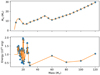 |
Fig. 1. Relation between zero-age main-sequence mass and ejecta mass of non-rotating core-collapse supernova progenitors at solar metallicity in the GENEVA library (Ekström et al. 2012) and the relation between the zero-age main-sequence mass and the explosion energy (Sukhbold et al. 2016). The blue dots show the calculated points, while the orange lines show the interpolation between them. |
As the explosion energy Eej is not provided by stellar evolutionary calculations but requires additional calculations taking them as initial conditions, we used the results of Sukhbold et al. (2016); they provide an M⋆ − Eej law in Table 5, which is referred to as model N20K based on neutrino-powered explosions and makes it possible to interpolate the explosion energy from the progenitor mass. These data are displayed in Fig. 1 (bottom).
Using these ejecta-mass and explosion energy distributions described above, as well as the uniform age distribution, the SNRs are placed throughout the Milky Way according to one of the following papers: Faucher-Giguère & Kaspi (2006), Steiman-Cameron et al. (2010), Green (2015), or Reid et al. (2019). The source distributions will be called CAFG, Steiman-Cameron, Green, and Reid from here on and are described in more detail in Sect. 2.2.2. The Steiman-Cameron and Green models are both implemented following the work by Steppa & Egberts (2020). In this work, we used a galactocentric coordinate system with the Sun located at x = 0, y = 8.5 kpc, z = 0.
2.2.2. Spatial distribution of SNRs
The CAFG model. The four-spiral-arm model described in Faucher-Giguère & Kaspi (2006) is used to model pulsar positions. We use it by imposing that the birth locations of the supernovae follow the radial distribution described for the pulsars and that the arm be chosen at random. The locations of the supernovae also follow a z distribution, with thermonuclear supernovae following the HI gas density and core-collapse supernovae following the HII gas density. The radial distribution of sources uses the following probability density function:
![Mathematical equation: $$ \begin{aligned} \rho (r) = A \left(\frac{r+R_1}{R_{\odot }+R1} \right)^{a} {\exp } \left[-b\left(\frac{r-R_{\odot }}{R_{\odot }+R_1}\right)\right], \end{aligned} $$](/articles/aa/full_html/2024/07/aa49779-24/aa49779-24-eq46.gif) (28)
(28)
where A is a normalisation constant, r is the galactocentric radius, R1 = 0.55 kpc, a = 1.64, and b = 0.24.
The Steiman-Cameron model. A four-spiral-arm model based on the interstellar medium is described in Steiman-Cameron et al. (2010). The model matches the data obtained by the FIRAS instrument of the Cosmic Background Explorer for the [CII] 158 μm and [NII] 205 μm lines of the interstellar medium. The distribution of sources is described by the following probability density equation:
 (29)
(29)
where σr is the scale length of the radius, R is the local maximum radius, δ is the azimuthal scale angle, βi is the pitch angle of the arm, ai is the orientation of the arm and σz, 2 is the scale height. The parameters for the arms can be seen in Table 1.
Parameter values for Steiman-Cameron arms.
The Green model. An azimuthally symmetric model based on SNR data is described in Green (2015). The spatial distribution we use is described by the following probability density function:
 (30)
(30)
with R⊙ being the distance of the Sun to the Galactic centre, z0 the scale height of the Galactic disc, α the shape parameter, and β the rate parameter. The parameter roff accounts for a non-zero density at r = 0. Following Steppa & Egberts (2020), we set z0 = 0.083 kpc, roff = 0 kpc, α = 1.09, and β = 3.87.
The Reid model. A four-spiral-arm model based on data from massive stars with maser parallaxes is described in Reid et al. (2019). This model also includes some additional features: the Local Arm; a 3 kpc arm around the centre of the Galaxy; and an outer arm, which connects with the Norma Arm. The Local Arm is described as an arm segment and does not link with any of the other arms. The 3 kpc arm is associated with the Galactic bar and might not be a true spiral arm. The spiral arms are described by Eq. (31) and Table 2:
 (31)
(31)
Parameter values for arms in the Reid distribution of sources.
where R is the galactocentric radius at azimuth β, Rkink is the radius of the kink in the arm at azimuth βkink, and ψ is the pitch angle.
2.3. The gas distribution
For the matter distribution we need to know the hydrogen density of the region we place our sources into. In this work, we used the matter distribution described by Shibata et al. (2010), which includes an empirical model for the matter distribution. They describe the gas density of interstellar hydrogen (HI and H2) as a function of galactocentric distance and height above or below the Galactic plane. This empirical model closely matches the one used in the GALPROP code (Strong & Moskalenko 1998).
3. Confronting our simulated populations with available H.E.S.S. data
Following the modelling described in Sect. 2, we can simulate the Galactic population of SNRs. The typical parameters of interest are:
-
Kep: the electron-to-proton ratio.
-
α: the spectral index of the accelerated particles.
-
TST: the duration of the ST phase.
-
η: the CR acceleration efficiency.
-
The spatial distribution of sources.
We typically compute 100 realisations for a given set of parameters to ensure the stability of our results. We Note that the positions of simulated SNRs change for each of the 100 realisations for a given set of properties, but these 100 different position sets are constant when changing the population properties other than the source distribution model. This allows us to closely examine how each of the properties affects the population.
For each source, using the gamma-ray luminosity, size, and position we are able to determine whether it would have been detected in the HGPS. To account for the selection bias in the H.E.S.S. catalogue we followed the work in Steppa & Egberts (2020); in particular, we accounted for the fact that the HGPS sensitivity varies with position and source extent. For a simulated source to be detectable it must exceed the threshold of 5σ above the background. This condition reads
 (32)
(32)
where Fmin, 0 is the point-source sensitivity, θsource is the source extent (radius) and θPSF is the size of the H.E.S.S. point-spread function. The limited field of view of H.E.S.S. combined with the applied technique of deriving background measurements means that sources ≳1° are not detectable. It is worth noting that the source in the HGPS with the largest extent, Vela Junior, was the subject of a dedicated analysis rather than the analysis method used in the HGPS. Vela Junior has an extent of 1°; the largest extent of any source analysed using the method in the HGPS is Vela X, with an extent of 0.58°. Another well-known SNR, RX J1713.7−3946 was also the subject of a dedicated analysis and has an extent of 0.5°. In Fig. 2, the HGPS detectability range for point-like sources with a luminosity of 5 × 1033 photons s−1 is displayed, demonstrating the large variations in sensitivity as a function of Galactic longitude. This variation in sensitivity shows why it is not sufficient to have a cut-off in the integrated flux to determine if a source is detectable, and thus why we need to include the sensitivity of H.E.S.S. when testing each simulated source.
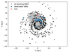 |
Fig. 2. Example of one realisation of a simulation of the population of Galactic SNRs. The grey shaded region is the HGPS detectability range for point-like sources with a luminosity of 5 × 1033 photons s−1 (equivalent to a differential flux at 1 TeV of ∼4 × 10⁻¹¹ TeV−1 cm−2 s−1 at a distance of 1 kpc). The blue plus symbols mark the simulated sources that are detectable, and the black dots mark the simulated sources that are not detectable. 3.7% of the emitting SNRs are detectable in this realisation. The location of the Sun is marked by the red cross. |
Because many of the HGPS sources are unidentified and at least some of those should be SNRs, we create an upper and lower limit for the HGPS sources we compare to. The lower limit is the firmly identified SNRs in the HGPS (8), and the upper limit includes all the unidentified sources (47) and the sources identified as composite SNRs (8); this gives us an upper limit of 63 sources to compare to. Moreover, only 12 of the unidentified sources have been found with a position compatible with a known SNR: this allows us to consider a more stringent upper limit of 28 sources. Of the eight firmly detected SNRs, which have been modelled individually (H.E.S.S. Collaboration 2011, 2015, 2018b,c,d,e; Nguyen-Dang et al. 2023; Cui et al. 2018), four of them are clearly found with Emax > 10 TeV, two of them with Emax ∼ 10 TeV and, two of them with Emax < 10 TeV. We use this as an additional constraint on the populations.
4. Results
We compare our synthetic populations to the HGPS sample. For illustrative purposes, we define a reference set of parameters as follows: the Steiman-Cameron source distribution, the Bell method to estimate pmax, α = 4.3, Kep = 10−3, η = 7%, and TST = 20 kyr. It is important to note that this particular set of properties is not the only set that can describe the data, but it is a useful starting point for making comparisons.
The effect of varying α from 4.0 to 4.4 is shown in Fig. 3. In this case, only one of the sets of parameters (with a spectral index of 4.3) is found in agreement with the data. With a spectral index of 4.3, almost all (96%) the populations fit between the eight firmly detected SNRs (blue line) and the stringent upper limit (28), which only includes sources associated with SNRs (green line). All the populations for this parameter set fit between the eight firmly detected SNRs (blue line) and the strict upper limit, which includes all the unidentified sources (orange line). For α > 4.3, there are too few detectable SNRs, while α < 4.3 overproduces the H.E.S.S. results. The log N − log S distribution of fluxes for the simulated SNRs has a very similar shape to that of the H.E.S.S. SNRs. Harder spectra (α close to 4) increase the number of detectable SNRs, which is expected since harder spectra correspond to an increase in the flux in the TeV range, thus increasing the horizon of detectability. The total number of SNRs remains the same for all the values of the spectral index (right panel Fig. 3).
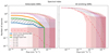 |
Fig. 3. log N − log S distribution of detectable SNRs (left) and all emitting SNRs (right) based on 100 Monte Carlo realisations following a Steiman-Cameron source distribution, Emax estimation considering Bell instabilities, Kep = 10−3.0, and η = 7%. The spectral index of the accelerated particles α varies from 4 to 4.4. Shaded areas indicate ± one standard deviation. Thick solid lines correspond to the HGPS limits (blue: identified SNRs; green: identified and unidentified sources associated with SNRs; orange: all unidentified sources). The hatched region shows the ideal region for the simulated SNRs: between the identified SNRs and the sources associated with SNRs. |
Changing the efficiency, η, from 1% to 10% directly impacts the number of detectable SNRs, as shown in Fig. 4. With our benchmark case, we find that η < 5% and η > 9% seem to under- or over-produce the H.E.S.S. data, respectively.
Exploring values of Kep in the 10−2 to 10−5 range, we illustrate in Fig. 5 that a value of 10−3.5 leads to results compatible within the firmly detected H.E.S.S. SNRs and our stringent upper limit. With the initial benchmark set of parameters we considered, a value of Kep = 10−2.5 leads to a simulated population of SNRs close to the upper limit of all the unknown H.E.S.S. sources; thus, this is a possible but extreme and quite unlikely case.
Figure 6 shows the mean hadronic ratio (ratio of the number of SNRs with gamma-ray luminosity dominated by the hadronic component to the total number of SNRs) against the integrated flux (> 1 TeV) of the detectable SNRs using the same cumulative binning as in Figs. 3–5 and its strong dependence on the parameters Kep, η, and α. The dependence on Kep is easily understood since this parameter directly affects the normalisation of the electron spectrum, and thus an increase in Kep leads to a decrease of the hadronic ratio (increase in the number of leptonic-dominated SNRs), which can be seen in Fig. 6 (top left). At higher integrated fluxes, we have fewer detectable SNRs. For Kep = 10−4 and Kep = 10−5 we have, on average, < 1 of the brightest SNRs. As seen in Fig. 5, this brightest detectable SNR is always dominated by hadronic emission, and this is why there is no statistical error at the edge of Fig. 6. An increase in η, a decrease in α, or both also leads to a decrease of the hadronic ratio (increase of the number of leptonic dominated SNRs). This can be understood as the result of several combined effects: by decreasing α, increasing η, or both, in a given horizon, we allow for a part of the SNR population (older SNRs, or those located in less dense parts) to become detectable, and thus we unveil a part of the SNR population that is typically more leptonic dominated (see Table 3), on top of the already detected hadronic SNRs. This leads to a decrease in the hadronic ratio.
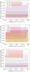 |
Fig. 6. Mean ratio of hadronic-dominated detectable SNRs versus integrated flux, as in Fig. 3. Top left panel illustrates the importance of Kep (fixing α = 4.3 and η = 7%); top right panel illustrates the effect of varying η (fixing Kep = 10−3 and α = 4.3); and bottom panel illustrates the effect of varying α (fixing η = 7% and Kep = 10−3). The rest of the properties are as in Fig. 3. |
Typical characteristics of detectable SNRs in the simulated populations.
We additionally investigate the influence of the duration of the active acceleration phase, treating the duration of the ST phase TST as a free parameter that we are artificially changing. Changes within a factor of a few typically do not affect our results substantially, as shown in Fig. 7. This is somewhat expected since mostly young ≲5 − 10 kyr old SNRs account for the brightest TeV SNRs.
Diffusive shock reacceleration, as discussed in Sect. 2.1.2, is found to be especially relevant at old (≳10 kyr) SNR shocks (Bell 1978; Blasi 2004, 2017) and for small α; this does not substantially impact our results in the TeV range.
The different spatial distributions of SNRs are compared in Fig. 8. The importance of the source distribution is highlighted in the fact that the differences in the number of the detectable sub-sample of sources between the spatial distributions (left panel) is larger than when considering all emitting sources (right panel). At the same time, this shows that a thorough discussion on the spatial model requires taking into account the refined description of the sensitivity of the instrument, including its spatial dependence, as done in this work. Interestingly, the Steiman-Cameron and the Green distributions produce very similar detectable simulated SNRs despite having very different source distributions. All spatial distributions considered can account for the HGPS data when adjusting the other parameters of the SNR population.
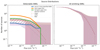 |
Fig. 8. As in Fig. 3, fixing α = 4.3 and varying the source distribution models: Stemian-Cameron, CAFG, Green, and Reid. |
Systematic exploration of the parameter space. In addition to varying each parameter at a time for the benchmark case discussed above, we performed a systematic exploration of the parameter space with 4.0 ≤ α ≤ 4.4, 10−5 ≤ Kep ≤ 10−2 and 0.01 ≤ η ≤ 0.1, considering Emax from the Bell and Hillas estimates. For these simulated properties, the maximum length of the ST phase was set to 20 kyr, and the Steiman-Cameron source distribution were used.
Exploring the parameter space, we constrained the results of our simulations by the HGPS catalogue, especially investigating which parameters can lead to realisations compatible with the detected Galactic population.
Moreover, we check that the maximum energy of accelerated particles, Emax, at the simulated SNRs is compatible with the current Emax estimated from the measured gamma-ray differential spectrum at each Galactic SNR. Schematically, out of the eight firmly detected SNRs, four of them are clearly found with Emax > 10 TeV (HESS J0852−463, HESS J1442−624, HESS J1713.7−3946 and HESS J1731−347), two of them with Emax ∼ 10 TeV (HESS J1534−571 and HESS J1718−347). We should mention that the cases of HESS J1801−233 (W28; Cui et al. 2018) and HESS J1911+090 (W49B; H.E.S.S. Collaboration 2018d) are rather tricky, as these two sources are thought to be SNRs interacting with molecular clouds, so it is not easy to ascribe the gamma-ray emission to the SNR shock, to clouds, or to a combination of the two. In addition, the question of whether there is an actual exponential suppression in the gamma-ray flux is yet not clearly answered. It remains that the gamma-ray luminosity is steeply decreasing in the ∼1 − 10 TeV range, and we considered that Emax < 10 TeV in this work.
For all realisations of our simulations, we checked the number of realisations for which (1) results are found between the firmly detected H.E.S.S. SNRs (8) and all the detected H.E.S.S. sources associated with SNRs (28); and (2) the Emax of the simulated SNRs that are detectable in our sample is compatible with the number of SNRs with Emax > 10 TeV in the HGPS (≥4). This is illustrated in Fig. 9, where, assuming an Emax following Bell, one realisation of a simulated population is shown in the parameter space of the SNR age and Emax. The population parameters are chosen such that they lead to the best agreement with HGPS data (α = 4.2, Kep = 10−5, η = 9%, with ∼97% of the realisations compatible with data). Interestingly, in this situation, the number of SNR PeVatrons (accelerating particles up to the PeV range) is close to zero, which would be compatible with the idea that PeV CRs are not accelerated at typical SNRs (Cristofari et al. 2020). The prescription of Hillas naturally leads to possible higher values of Emax, but it does not substantially increase the chances of detecting a SNR PeVatron; this can be seen in Fig. 10.
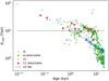 |
Fig. 9. Maximum energy of accelerated protons versus age of each simulated SNR for a given Monte Carlo realisation. Parameters adopted are α = 4.2, Kep = 10−5, η = 9%, and with Emax following the Bell prescription. The horizontal line at 10 TeV illustrates the criterion required to account for the HGPS data. |
The results are illustrated in Figs. 11 and 12. In Fig. 11, the results are displayed assuming Emax follows the Bell description. In Fig. 12, we show the results with Emax estimated using the Hillas criterion.
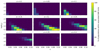 |
Fig. 11. Two-dimensional histogram plots showing the percentage of populations that have at least as many detectable simulated SNRs as firmly detected H.E.S.S. SNRs, do not exceed the number of H.E.S.S. sources associated with SNRs, and they have at least as many detectable SNRs with Emax ≥ 10 TeV as HGPS SNRs. The source distribution is Steiman-Cameron, and Emax follows the Bell description. |
It follows from Fig. 11 that one can rule out the following parameters: α ≳ 4.35 and Kep > 10−3. One can only find a set of parameters for which > 80% of the realisations are within the associated SNR limits if 4.1 ≲ α < 4.3, Kep < 10−3.5, and η > 0.02. However, Fig. 12 illustrates that when the Emax is estimated with the Hillas criterion, if α < 4.15, or if Kep > 10−3 no region of the parameter space can account for the HGPS data. The lower limit placed on α is a direct result of including the emission from reaccelerated particles in our SNR model. This emission is larger at smaller α and causes the populations with those parameters to have more detectable SNRs than the HGPS. In both plots, the correlations between parameters can be seen: an increase in η is compensated by either a decrease in Kep or larger values of α. This intertwining makes it arduous to identify a preferred region of the parameter space.
The systematic exploration of the parameter space allows us to identify the set of parameters that lead to a maximum number of realisations in agreement with the HGPS data (see for example Figs. 11 and 12), but also to examine the properties of these synthetic populations. Assuming an Emax following Bell, the typical characteristics of the simulated population for which a maximum number of Monte Carlo realisations are in agreement with the HGPS are shown in Table 3.
A few remarks are in order. The set of parameters leading to the highest fraction of realisations in agreement with the HGPS is α = 4.2, Kep = 10−5, η = 0.09. For all populations leading to 90% of compatibility with the HGPS, we found that 4.2 ≳ α ≳ 4.1 and 10−4.5 ≳ Kep ≳ 10−5 for a CR efficiency 0.1 ≳ η ≳ 0.03. Interestingly, the electron-to-proton ratio Kep is found to be on the lower side of typically inferred values, and at the same time, typically about 40%−60% of the gamma-ray emission of the simulated SNRs detectable in the survey is dominated by leptonic interactions (see hadronic ratio). This is somehow counter-intuitive, as the idea that the VHE gamma-ray emission of SNRs is leptonic usually implies that the acceleration of leptons is efficient. In our case, low values of Kep are compensated by sufficiently hard spectra and efficiencies, to allow for leptonic-dominated gamma rays to be detectable. The leptonic-dominated SNRs are typically older than the hadronic-dominated SNRs (the mean age of leptonic ones is typically twice the mean age of hadronic ones), which is consistent with the consensual picture (Pohl 1996; Reynolds 2008; Acero et al. 2015), for instance because of the reduced efficiency of magnetic-field amplification at slower shocks, thus reducing losses suffered by electrons. As illustrated in Fig. 6, the efficiency of particle acceleration is indeed found to strongly impact the fraction of leptonic sources. Indeed, the spectra of both accelerated protons and electrons are directly proportional to the acceleration efficiency, but an increase of the efficiency allows for the dimmer leptonic-dominated sources to reach the sensitivity of the HGPS, and thus unveils the leptonic-dominated SNRs. With α = 4.3, and Kep = 10−3, varying the CR efficiency from 0.01 to 0.1 changes the fraction of hadronic sources from ≈1 to ≈0.2. It should be noted that this outcome was achieved assuming that the maximum energy at SNRs is determined by the development of non-resonant streaming instabilities, and ensuring that the count of simulated SNRs detected above approximately 10 TeV aligns with the HGPS data. Considering a maximum energy determined by the Hillas criterion, or relaxing the constraint on the number of SNRs detected above about 10 TeV, opens up a wider range of possibilities where parameter combinations with an α value around 4.4 or a Kep value around 10−2 can be identified. Both population (Ellison et al. 2007; Cristofari et al. 2013) and theoretical studies (Corso et al. 2023) have not yet led to stringent constraints for the values of Kep or the ratio of hadronic-dominated sources. Mandelartz & Becker Tjus (2015) interpreted 21 out of 24 SNRs in the GeV range as hadronic dominated, but the work of Zeng et al. (2019) led to more complex discussions.
5. Conclusion
Relying on a Monte Carlo approach, we simulated populations of the Galactic SNRs in the TeV range (built on a physically motivated model of the gamma-ray emission from accelerated protons and electrons at SNR shocks) and confronted the results of the simulated populations to available data from the systematic survey of the Galactic plane performed by H.E.S.S.
We performed a systematic exploration of the parameter space defined by Kep, which is the electron-to-proton ratio; α, the power-law spectral index of the accelerated particles at the SNR shocks; TST, the duration of the ST phase; and η, the CR acceleration efficiency. We did this considering different prescriptions for the description of the maximum energy of accelerated particles Emax and different prescriptions for the spatial distribution of sources. Our conclusions are listed below.
-
We find that the Galactic population of TeV SNRs can be explained by multiple regions of the parameter space. Given the current population in the HGPS, only some parts of the parameter space seem to be excluded. For instance, α ≲ 4.05 seems to be disfavoured in all cases. Kep ≳ 10−2.5, is excluded and Kep ∼ 10−3 requires α ≳ 4.35 and η ≲ 0.02.
-
Despite the limitations of our approach, the systematic exploration of the parameter space allows us to look for the region of the parameter space producing the most realisations within the limits of the HGPS sample. In addition to the requirement concerning the total number of sources, the additional constraint on the maximum energy (ensuring that Emax at SNRs is compatible with values estimated at individual SNRs) allows us to further reduce the allowed parameter space. One possible solution rendering ∼97% populations in the limits of the HGPS is α = 4.2, Kep = 10−5, η = 9%, assuming Emax from the Bell prescription. In this case, the mean ratio of hadronic-to-leptonic-dominated SNRs is 0.62, which is compatible with the current idea that the TeV emission can be leptonic or hadronic for the different known SNRs. We note that the relatively high efficiency η = 9% allows for a non-negligible fraction of leptonic SNRs, which are older or located in low-density, regions to be detectable.
-
The sets of parameters that have ≳90% realisations compatible with the HGPS are obtained with 4.1 ≲ α ≲ 4.2, 10−5 ≲ Kep ≲ 10−4.5 and 0.03 ≲ η ≲ 0.1. Interestingly, this leads to a fraction of ≈40 − 60% of leptonic-dominated SNRs in the TeV range, along with a reduced fraction of electrons injected at the SNR shocks. This means that our study naturally highlights situations in which we can account for a significant (∼50%) fraction of the sources being dominated by the leptonic emission, with a low value of Kep (∼10−5). For most SNRs, the dominant processes at play (leptonic vs. hadronic) are still debated, and thus the overall situation for the Galactic population is also unknown (see, for example discussion in Zeng et al. 2019). In fact, even for what is probably the best-studied SNR of the TeV range RX J1713−3946, numerous works have still not managed to conclude on the dominant mechanism at play (Ellison et al. 2010; Zirakashvili & Aharonian 2010; Morlino & Caprioli 2012; Gabici 2017; Ohira & Yamazaki 2017; Cristofari et al. 2021b; Fujita et al. 2022). In other words, the simulated populations are thus directly compatible with a situation where half of the TeV-detected SNRs are leptonic dominated, and at the same time the fraction of injected electrons at SNR shocks is substantially lower than the ∼1/100 (∼1/50) electron-to-proton ratio measured in the local CR spectrum approximately in the giga-electron-volt range. This would thus be an additional argument in favour of SNRs not being dominant sources of CR electrons (Gabici et al. 2019; Lipari 2019), and at the same time, that a substantial fraction of SNRs are detected in the TeV range with a dominant leptonic component. We note that this result was obtained under the assumption that the maximum energy at SNRs is set by the growth of non–resonant streaming instabilities, and ensuring that the number of simulated SNRs detected above ≳10 TeV is compatible with the HGPS data. Considering a maximum energy set by the Hillas criterion or relaxing the condition on the number of SNRs detected above ≳10 TeV leads to more diverse possibilities where sets of parameters with α ∼ 4.4 or Kep ∼ 10−2 can be found.
-
Some parameters do not substantially affect our results. For TST this is coherent with the idea that most TeV-emitting SNRs are young (≲a few thousand years). The various prescriptions for the spatial distribution of sources do not substantially affect our results.
Any additional constraint on one of the parameters explored in our study would naturally narrow down the parameter space compatible with the HGPS. Moreover, an increase in the sample of the firm SNR detections (8, our lower limit) would help our approach. This increased number of detections is clearly expected with next-generation instruments such as the CTAO (Cristofari et al. 2017; Cherenkov Telescope Array Consortium 2019; CTA Consortium 2023) or LHAASO (Liu et al. 2016). Cristofari et al. (2017), CTA Consortium (2023) discussed that CTAO could detect up to several hundreds of SNRs in the systematic exploration of the sky.
Additionally, joint observations of SNRs with next-generation radio observatories (Jonas & MeerKAT Team 2016; Tingay et al. 2013; Dewdney et al. 2009) will provide data of unprecedented value concerning the content of non-thermal electrons accelerated at SNR shocks and help disentangle the hadronic and leptonic content, thus allowing us to better understand the details of DSA at SNRs.
Acknowledgments
This work has been funded by the Deutsche Forschungsgemeinschaft (DFG, German Research Foundation) with the grant 500120112 and supported by the grant PID2021-124581OB-I00 funded by MCIN/AEI/10.13039/501100011033 and 2021SGR00426 of the Generalitat de Catalunya. This work was also supported by the Spanish program Unidad de Excelencia María de Maeztu CEX2020-001058-M. P.C. acknowledges support from the PSL Starting Grant GALAPAGOS. The authors gratefully acknowledge the computing time made available to them on the high-performance computer “Lise” at the NHR Center NHR@ZIB. This center is jointly supported by the Federal Ministry of Education and Research and the state governments participating in the NHR (https://www.nhr-verein.de/unsere-partner).
References
- Acciari, V. A., Aliu, E., Arlen, T., et al. 2011, ApJ, 730, L20 [NASA ADS] [CrossRef] [Google Scholar]
- Acero, F., Lemoine-Goumard, M., Renaud, M., et al. 2015, A&A, 580, A74 [NASA ADS] [CrossRef] [EDP Sciences] [Google Scholar]
- Acero, F., Ackermann, M., Ajello, M., et al. 2016, ApJS, 224, 8 [NASA ADS] [CrossRef] [Google Scholar]
- Adriani, O., Barbarino, G. C., Bazilevskaya, G. A., et al. 2011, Science, 332, 69 [NASA ADS] [CrossRef] [Google Scholar]
- Albert, J., Aliu, E., Anderhub, H., et al. 2007, ApJ, 664, L87 [NASA ADS] [CrossRef] [Google Scholar]
- Bell, A. R. 1978, MNRAS, 182, 443 [Google Scholar]
- Bell, A. R., Schure, K. M., Reville, B., & Giacinti, G. 2013, MNRAS, 431, 415 [Google Scholar]
- Bisschoff, D., Potgieter, M. S., & Aslam, O. P. M. 2019, ApJ, 878, 59 [NASA ADS] [CrossRef] [Google Scholar]
- Blasi, P. 2004, Astropart. Phys., 21, 45 [NASA ADS] [CrossRef] [Google Scholar]
- Blasi, P. 2017, MNRAS, 471, 1662 [NASA ADS] [CrossRef] [Google Scholar]
- Blondin, J. M., Wright, E. B., Borkowski, K. J., & Reynolds, S. P. 1998, ApJ, 500, 342 [Google Scholar]
- Brott, I., de Mink, S. E., Cantiello, M., et al. 2011a, A&A, 530, A115 [NASA ADS] [CrossRef] [EDP Sciences] [Google Scholar]
- Brott, I., Evans, C. J., Hunter, I., et al. 2011b, A&A, 530, A116 [NASA ADS] [CrossRef] [EDP Sciences] [Google Scholar]
- Castor, J., McCray, R., & Weaver, R. 1975, ApJ, 200, L107 [NASA ADS] [CrossRef] [Google Scholar]
- Cherenkov Telescope Array Consortium (Acharya, B. S., et al.) 2019, Science with the Cherenkov Telescope Array (World Scientific Publishing Co.) [Google Scholar]
- Chevalier, R. A. 1982, ApJ, 258, 790 [NASA ADS] [CrossRef] [Google Scholar]
- Choi, J., Dotter, A., Conroy, C., et al. 2016, ApJ, 823, 102 [Google Scholar]
- Corso, N. J., Diesing, R., & Caprioli, D. 2023, ApJ, 954, 1 [NASA ADS] [CrossRef] [Google Scholar]
- Cristofari, P. 2021, Universe, 7, 324 [NASA ADS] [CrossRef] [Google Scholar]
- Cristofari, P., & Blasi, P. 2019, MNRAS, 489, 108 [NASA ADS] [CrossRef] [Google Scholar]
- Cristofari, P., Gabici, S., Casanova, S., Terrier, R., & Parizot, E. 2013, MNRAS, 434, 2748 [Google Scholar]
- Cristofari, P., Gabici, S., Humensky, T. B., et al. 2017, MNRAS, 471, 201 [NASA ADS] [CrossRef] [Google Scholar]
- Cristofari, P., Blasi, P., & Amato, E. 2020, Astropart. Phys., 123, 102492 [Google Scholar]
- Cristofari, P., Blasi, P., & Caprioli, D. 2021a, A&A, 650, A62 [NASA ADS] [CrossRef] [EDP Sciences] [Google Scholar]
- Cristofari, P., Niro, V., & Gabici, S. 2021b, MNRAS, 508, 2204 [NASA ADS] [CrossRef] [Google Scholar]
- CTA Consortium 2023, ArXiv e-prints [arXiv:2310.02828] [Google Scholar]
- Cui, Y., Yeung, P. K. H., Tam, P. H. T., & Pühlhofer, G. 2018, ApJ, 860, 69 [Google Scholar]
- Cummings, A. C., Stone, E. C., Heikkila, B. C., et al. 2016, ApJ, 831, 18 [CrossRef] [Google Scholar]
- Das, S., Brose, R., Meyer, D. M. A., et al. 2022, A&A, 661, A128 [NASA ADS] [CrossRef] [EDP Sciences] [Google Scholar]
- Dewdney, P. E., Hall, P. J., Schilizzi, R. T., & Lazio, T. J. L. W. 2009, IEEE Proc., 97, 1482 [Google Scholar]
- Dotter, A. 2016, ApJS, 222, 8 [Google Scholar]
- Eggenberger, P., Meynet, G., Maeder, A., et al. 2008, Ap&SS, 316, 43 [Google Scholar]
- Ekström, S., Georgy, C., Eggenberger, P., et al. 2012, A&A, 537, A146 [Google Scholar]
- Ellison, D. C., Patnaude, D. J., Slane, P., Blasi, P., & Gabici, S. 2007, ApJ, 661, 879 [NASA ADS] [CrossRef] [Google Scholar]
- Ellison, D. C., Patnaude, D. J., Slane, P., & Raymond, J. 2010, ApJ, 712, 287 [NASA ADS] [CrossRef] [Google Scholar]
- Faucher-Giguère, C.-A., & Kaspi, V. M. 2006, ApJ, 643, 332 [CrossRef] [Google Scholar]
- Ferrière, K. M. 2001, Rev. Mod. Phys., 73, 1031 [NASA ADS] [CrossRef] [Google Scholar]
- Finke, J. D., & Dermer, C. D. 2012, ApJ, 751, 65 [CrossRef] [Google Scholar]
- Fragos, T., Andrews, J. J., Bavera, S. S., et al. 2023, ApJS, 264, 45 [NASA ADS] [CrossRef] [Google Scholar]
- Fujita, Y., Yamazaki, R., & Ohira, Y. 2022, ApJ, 933, 126 [NASA ADS] [CrossRef] [Google Scholar]
- Gabici, S. 2017, AIP Conf. Ser., 1792, 020002 [NASA ADS] [Google Scholar]
- Gabici, S., Evoli, C., Gaggero, D., et al. 2019, Int. J. Mod. Phys. D, 28, 1930022 [CrossRef] [Google Scholar]
- Georgy, C. 2010, PhD Thesis, University of Geneva, Switzerland [Google Scholar]
- Green, D. A. 2015, MNRAS, 454, 1517 [NASA ADS] [CrossRef] [Google Scholar]
- Hess, V. F. 1912, Phys. Z., 13, 1084 [Google Scholar]
- H.E.S.S. Collaboration (Abramowski, A., et al.) 2011, A&A, 531, A81 [NASA ADS] [CrossRef] [EDP Sciences] [Google Scholar]
- H.E.S.S. Collaboration (Abramowski, A., et al.) 2015, A&A, 574, A100 [CrossRef] [EDP Sciences] [Google Scholar]
- H.E.S.S. Collaboration (Abdalla, H., et al.) 2018a, A&A, 612, A3 [NASA ADS] [CrossRef] [EDP Sciences] [Google Scholar]
- H.E.S.S. Collaboration (Abdalla, H., et al.) 2018b, A&A, 612, A7 [NASA ADS] [CrossRef] [EDP Sciences] [Google Scholar]
- H.E.S.S. Collaboration (Abramowski, A., et al.) 2018c, A&A, 612, A4 [NASA ADS] [CrossRef] [EDP Sciences] [Google Scholar]
- H.E.S.S. Collaboration (Abdalla, H., et al.) 2018d, A&A, 612, A5 [NASA ADS] [CrossRef] [EDP Sciences] [Google Scholar]
- H.E.S.S. Collaboration Abdalla, H., et al.) 2018e, A&A, 612, A6 [NASA ADS] [CrossRef] [EDP Sciences] [Google Scholar]
- Jonas, J., & MeerKAT Team 2016, MeerKAT Science: On the Pathway to the SKA, 1 [Google Scholar]
- Kafexhiu, E., Aharonian, F., Taylor, A. M., & Vila, G. S. 2014, Phys. Rev. D, 90, 123014 [Google Scholar]
- Khangulyan, D., Aharonian, F. A., & Kelner, S. R. 2014, ApJ, 783, 100 [Google Scholar]
- Kroupa, P. 2001, MNRAS, 322, 231 [NASA ADS] [CrossRef] [Google Scholar]
- Lipari, P. 2019, Phys. Rev. D, 99, 043005 [NASA ADS] [CrossRef] [Google Scholar]
- Liu, Y., Cao, Z., Chen, S., et al. 2016, ApJ, 826, 63 [NASA ADS] [CrossRef] [Google Scholar]
- Longair, M. S. 1994, High Energy Astrophysics. Volume 2: Stars, the Galaxy and the Interstellar Medium (Cambridge: Cambridge University Press) [Google Scholar]
- Mandelartz, M., & Becker Tjus, J. 2015, Astropart. Phys., 65, 80 [NASA ADS] [CrossRef] [Google Scholar]
- Meyer, D. M. A., & Meliani, Z. 2022, MNRAS, 515, L29 [NASA ADS] [CrossRef] [Google Scholar]
- Meyer, D. M. A., Mignone, A., Petrov, M., et al. 2021, MNRAS, 506, 5170 [NASA ADS] [CrossRef] [Google Scholar]
- Meyer, D. M. A., Velázquez, P. F., Petruk, O., et al. 2022, MNRAS, 515, 594 [CrossRef] [Google Scholar]
- Meyer, D. M. A., Pohl, M., Petrov, M., & Egberts, K. 2023, MNRAS, 521, 5354 [NASA ADS] [CrossRef] [Google Scholar]
- Morlino, G., & Caprioli, D. 2012, A&A, 538, A81 [NASA ADS] [CrossRef] [EDP Sciences] [Google Scholar]
- Nguyen-Dang, N. T., Pühlhofer, G., Sasaki, M., et al. 2023, A&A, 679, A48 [NASA ADS] [CrossRef] [EDP Sciences] [Google Scholar]
- Ohira, Y., & Yamazaki, R. 2017, J. High Energy Astrophys., 13, 17 [CrossRef] [Google Scholar]
- Pais, M., & Pfrommer, C. 2020, MNRAS, 498, 5557 [NASA ADS] [CrossRef] [Google Scholar]
- Paxton, B., Marchant, P., Schwab, J., et al. 2015, ApJS, 220, 15 [Google Scholar]
- Paxton, B., Schwab, J., Bauer, E. B., et al. 2018, ApJS, 234, 34 [NASA ADS] [CrossRef] [Google Scholar]
- Paxton, B., Smolec, R., Schwab, J., et al. 2019, ApJS, 243, 10 [Google Scholar]
- Pohl, M. 1996, A&A, 307, L57 [Google Scholar]
- Ptuskin, V. 2010, ApJ, 718, 31 [NASA ADS] [CrossRef] [Google Scholar]
- Ptuskin, V. S., & Zirakashvili, V. N. 2003, A&A, 403, 1 [NASA ADS] [CrossRef] [EDP Sciences] [Google Scholar]
- Ptuskin, V. S., & Zirakashvili, V. N. 2005, A&A, 429, 755 [NASA ADS] [CrossRef] [EDP Sciences] [Google Scholar]
- Reid, M. J., Menten, K. M., Brunthaler, A., et al. 2019, ApJ, 885, 131 [Google Scholar]
- Reynolds, S. P. 2008, ARA&A, 46, 89 [Google Scholar]
- Schure, K. M., & Bell, A. R. 2013, MNRAS, 435, 1174 [NASA ADS] [CrossRef] [Google Scholar]
- Schure, K. M., Bell, A. R., O’C Drury, L., & Bykov, A. M., 2012, Space Sci. Rev., 173, 491 [NASA ADS] [Google Scholar]
- Shibata, T., Ishikawa, T., & Sekiguchi, S. 2010, ApJ, 727, 38 [Google Scholar]
- Smartt, S. J., Eldridge, J. J., Crockett, R. M., & Maund, J. R. 2009, MNRAS, 395, 1409 [CrossRef] [Google Scholar]
- Steiman-Cameron, T. Y., Wolfire, M., & Hollenbach, D. 2010, ApJ, 722, 1460 [NASA ADS] [CrossRef] [Google Scholar]
- Steppa, C., & Egberts, K. 2020, A&A, 643, A137 [NASA ADS] [CrossRef] [EDP Sciences] [Google Scholar]
- Strong, A. W., & Moskalenko, I. V. 1998, ApJ, 509, 212 [NASA ADS] [CrossRef] [Google Scholar]
- Sukhbold, T., Ertl, T., Woosley, S. E., Brown, J. M., & Janka, H. T. 2016, ApJ, 821, 38 [NASA ADS] [CrossRef] [Google Scholar]
- Sushch, I., Brose, R., & Pohl, M. 2018, A&A, 618, A155 [NASA ADS] [CrossRef] [EDP Sciences] [Google Scholar]
- Szécsi, D., Agrawal, P., Wünsch, R., & Langer, N. 2022, A&A, 658, A125 [NASA ADS] [CrossRef] [EDP Sciences] [Google Scholar]
- Tingay, S. J., Goeke, R., Bowman, J. D., et al. 2013, PASA, 30, e007 [Google Scholar]
- Truelove, J. K., & McKee, C. F. 1999, ApJS, 120, 299 [Google Scholar]
- van Veelen, B., Langer, N., Vink, J., García-Segura, G., & van Marle, A. J. 2009, A&A, 503, 495 [NASA ADS] [CrossRef] [EDP Sciences] [Google Scholar]
- Vannoni, G., Gabici, S., & Aharonian, F. A. 2009, A&A, 497, 17 [CrossRef] [EDP Sciences] [Google Scholar]
- Völk, H. J., Berezhko, E. G., & Ksenofontov, L. T. 2005, A&A, 433, 229 [NASA ADS] [CrossRef] [EDP Sciences] [Google Scholar]
- Weaver, R., McCray, R., Castor, J., Shapiro, P., & Moore, R. 1977, ApJ, 218, 377 [Google Scholar]
- Zabalza, V. 2015, Proc. Int. Cosm. Ray Conf., 2015, 922 [Google Scholar]
- Zeng, H., Xin, Y., & Liu, S. 2019, ApJ, 874, 50 [NASA ADS] [CrossRef] [Google Scholar]
- Zirakashvili, V. N., & Aharonian, F. A. 2010, ApJ, 708, 965 [NASA ADS] [CrossRef] [Google Scholar]
- Zirakashvili, V. N., & Ptuskin, V. S. 2012, Astropart. Phys., 39, 12 [Google Scholar]
All Tables
All Figures
|
Fig. 1. Relation between zero-age main-sequence mass and ejecta mass of non-rotating core-collapse supernova progenitors at solar metallicity in the GENEVA library (Ekström et al. 2012) and the relation between the zero-age main-sequence mass and the explosion energy (Sukhbold et al. 2016). The blue dots show the calculated points, while the orange lines show the interpolation between them. |
| In the text | |
|
Fig. 2. Example of one realisation of a simulation of the population of Galactic SNRs. The grey shaded region is the HGPS detectability range for point-like sources with a luminosity of 5 × 1033 photons s−1 (equivalent to a differential flux at 1 TeV of ∼4 × 10⁻¹¹ TeV−1 cm−2 s−1 at a distance of 1 kpc). The blue plus symbols mark the simulated sources that are detectable, and the black dots mark the simulated sources that are not detectable. 3.7% of the emitting SNRs are detectable in this realisation. The location of the Sun is marked by the red cross. |
| In the text | |
|
Fig. 3. log N − log S distribution of detectable SNRs (left) and all emitting SNRs (right) based on 100 Monte Carlo realisations following a Steiman-Cameron source distribution, Emax estimation considering Bell instabilities, Kep = 10−3.0, and η = 7%. The spectral index of the accelerated particles α varies from 4 to 4.4. Shaded areas indicate ± one standard deviation. Thick solid lines correspond to the HGPS limits (blue: identified SNRs; green: identified and unidentified sources associated with SNRs; orange: all unidentified sources). The hatched region shows the ideal region for the simulated SNRs: between the identified SNRs and the sources associated with SNRs. |
| In the text | |
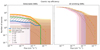 |
Fig. 4. As in Fig. 3, fixing α = 4.3 and varying η in the 1%–10% range. |
| In the text | |
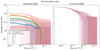 |
Fig. 5. As in Fig. 3, fixing α = 4.3 and varying the electron-proton ratio in the 10−2 − 10−5 range. |
| In the text | |
|
Fig. 6. Mean ratio of hadronic-dominated detectable SNRs versus integrated flux, as in Fig. 3. Top left panel illustrates the importance of Kep (fixing α = 4.3 and η = 7%); top right panel illustrates the effect of varying η (fixing Kep = 10−3 and α = 4.3); and bottom panel illustrates the effect of varying α (fixing η = 7% and Kep = 10−3). The rest of the properties are as in Fig. 3. |
| In the text | |
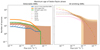 |
Fig. 7. As in Fig. 3, fixing α = 4.3 and varying TST from 5 kyr to 100 kyr. |
| In the text | |
|
Fig. 8. As in Fig. 3, fixing α = 4.3 and varying the source distribution models: Stemian-Cameron, CAFG, Green, and Reid. |
| In the text | |
|
Fig. 9. Maximum energy of accelerated protons versus age of each simulated SNR for a given Monte Carlo realisation. Parameters adopted are α = 4.2, Kep = 10−5, η = 9%, and with Emax following the Bell prescription. The horizontal line at 10 TeV illustrates the criterion required to account for the HGPS data. |
| In the text | |
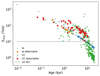 |
Fig. 10. As in Fig. 9, but with Emax following the Hillas prescription. |
| In the text | |
|
Fig. 11. Two-dimensional histogram plots showing the percentage of populations that have at least as many detectable simulated SNRs as firmly detected H.E.S.S. SNRs, do not exceed the number of H.E.S.S. sources associated with SNRs, and they have at least as many detectable SNRs with Emax ≥ 10 TeV as HGPS SNRs. The source distribution is Steiman-Cameron, and Emax follows the Bell description. |
| In the text | |
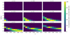 |
Fig. 12. As in Fig. 11, but with Emax estimated with the Hillas criterion. |
| In the text | |
Current usage metrics show cumulative count of Article Views (full-text article views including HTML views, PDF and ePub downloads, according to the available data) and Abstracts Views on Vision4Press platform.
Data correspond to usage on the plateform after 2015. The current usage metrics is available 48-96 hours after online publication and is updated daily on week days.
Initial download of the metrics may take a while.