| Issue |
A&A
Volume 687, July 2024
|
|
|---|---|---|
| Article Number | A130 | |
| Number of page(s) | 10 | |
| Section | The Sun and the Heliosphere | |
| DOI | https://doi.org/10.1051/0004-6361/202449774 | |
| Published online | 03 July 2024 | |
Filament eruption by multiple reconnections⋆
1
Shandong Provincial Key Laboratory of Optical Astronomy and Solar-Terrestrial Environment, and Institute of Space Sciences, Shandong University, Weihai 264209, PR China
e-mail: This email address is being protected from spambots. You need JavaScript enabled to view it.
2
Centre for mathematical Plasma Astrophysics, Dept. of Mathematics, KU Leuven, 3001 Leuven, Belgium
3
Observatoire de Paris, LESIA, Université PSL, CNRS, Sorbonne Université, Université de Paris, 5 Place Jules Janssen, 92190 Meudon, France
4
University of Glasgow, School of Physics and Astronomy, Glasgow, G12 8QQ Scotland, UK
5
Key Laboratory of Solar Activity, National Astronomical Observatories, Chinese Academy of Sciences, Beijing 100012, PR China
6
School of Astronomy and Space Science and Key Laboratory of Modern Astronomy and Astrophysics, Nanjing University, Nanjing 210023, PR China
Received:
28
February
2024
Accepted:
6
May
2024
Abstract
Context. Filament eruption is a common phenomenon in solar activity, but the triggering mechanism is not well understood.
Aims. We focus our study on a filament eruption located in a complex nest of three active regions close to a coronal hole.
Methods. The filament eruption is observed at multiple wavelengths: by the Global Oscillation Network Group (GONG), the Solar Terrestrial Relations Observatory (STEREO), the Solar Upper Transition Region Imager (SUTRI), and the Atmospheric Imaging Assembly (AIA) and Helioseismic and Magnetic Imager (HMI) on board the Solar Dynamic Observatory (SDO). Thanks to high-temporal-resolution observations, we were able to analyze the evolution of the fine structure of the filament in detail. The filament changes direction during the eruption, which is followed by a halo coronal mass ejection detected by the Large Angle Spectrometric Coronagraph (LASCO) on board the Solar and Heliospheric Observatory (SOHO). A Type III radio burst was also registered at the time of the eruption. To investigate the process of the eruption, we analyzed the magnetic topology of the filament region adopting a nonlinear force-free-field (NLFFF) extrapolation method and the polytropic global magnetohydrodynamic (MHD) modeling. We modeled the filament by embedding a twisted flux rope with the regularized Biot-Savart Laws (RBSL) method in the ambient magnetic field.
Results. The extrapolation results show that magnetic reconnection occurs in a fan-spine configuration resulting in a circular flare ribbon. The global modeling of the corona demonstrates that there was an interaction between the filament and open field lines, causing a deflection of the filament in the direction of the observed CME eruption and dimming area.
Conclusions. The modeling supports the following scenario: magnetic reconnection not only occurs with the filament itself (the flux rope) but also with the background magnetic field lines and open field lines of the coronal hole located to the east of the flux rope. This multiwavelength analysis indicates that the filament undergoes multiple magnetic reconnections on small and large scales with a drifting of the flux rope.
Key words: Sun: activity / Sun: coronal mass ejections (CMEs) / Sun: filaments, prominences / Sun: magnetic fields
Movies are available at https://www.aanda.org.
© The Authors 2024
 Open Access article, published by EDP Sciences, under the terms of the Creative Commons Attribution License (https://creativecommons.org/licenses/by/4.0), which permits unrestricted use, distribution, and reproduction in any medium, provided the original work is properly cited.
This article is published in open access under the Subscribe to Open model. This email address is being protected from spambots. You need JavaScript enabled to view it. to support open access publication.
1. Introduction
Solar filaments consist of relatively cold, dense plasma and are usually located above the polarity inversion lines (PILs; Babcock & Babcock 1955; Zirker 1989). When observed with Hα spectral lines on the solar disk, filaments appear as long dark structures, showing absorption characteristics. When they move to the limb of the Sun, they appear as bright emission features relative to the dark background, which is why they are often referred to as prominences (Ruan et al. 2018, 2019a). Filament eruptions are often associated with other forms of solar activity, such as solar flares, jets, and coronal mass ejections (CMEs).
The fine structure of the filaments can be analyzed thanks to high-resolution observations. Such images show that filaments are made of many parallel strands that are highly dynamic, showing a variety of flows. Zirker et al. (1998) observed counter-streaming along a prominence spine and barbs in Hα and detected these flows with speeds in the range of 5−20 km s−1. For active region filaments, during reconnection between strands, Hα blobs can be observed with similar velocities (Deng et al. 2002). During filament activity, counter-streaming in hotter plasma is also detected with velocities in the plane of the sky of between 70 and 100 km s−1 in 193 Å (Alexander et al. 2013). The flows of filament material must move along the magnetic field lines under the magnetic freezing effect. In this case, filament strands are bound by magnetic field lines, and so the direction of strands can often be used as a tracer of local magnetic field lines.
There are three general types of filament eruptions. The first type is failed eruptions (Liu et al. 2009; Kumar et al. 2011, 2023; Shen et al. 2011a; Joshi et al. 2022), where the filament cannot break free from the solar bond without accompanying CMEs. The second is partial eruptions (Tripathi et al. 2009; Gibson et al. 2006; Joshi et al. 2014; Schmieder et al. 2014; Bi et al. 2015; Cheng et al. 2018; Monga et al. 2021; Zhang et al. 2022a; Yang et al. 2023a), in which part of the filament falls back to the surface of the Sun while some manages to escape. The third is successful eruptions (Gilbert et al. 2007; Schrijver et al. 2008; Shen et al. 2012; Schmieder et al. 2013; Zhang et al. 2022b; Ruan et al. 2014, 2015), in which the filaments all explode away from the Sun and accompany the CMEs.
When the equilibrium state of a filament is destroyed by one or more factors, such as shear motion of the photosphere magnetic field (Sakai & Koide 1992), magnetic appearance and cancelation (Martin 1986), large-scale changes in the magnetic field structure of the corona (Low 1990), and so on, its magnetic field configuration can change, and this can trigger a filament eruption. In recent years, researchers have mainly divided the triggering mechanisms of the outbreak of filaments into two categories. One of these is magnetic reconnection (Su et al. 2007; Schmieder & Aulanier 2012; Schmieder et al. 2013, 2016; Chen et al. 2014, 2018; Zheng et al. 2017; Li et al. 2018; Hou et al. 2019, 2023; Ruan et al. 2019b; Yan et al. 2020; Chandra et al. 2021; Guo et al. 2021a; Hu et al. 2022; Koleva et al. 2022; Sun et al. 2023; Yang et al. 2023b; Xue et al. 2023). The ideal magnetohydrodynamic instabilities, such as kink instability (Gold & Hoyle 1960; Hood & Priest 1981) and torus instability (Kliem & Török 2006), are also considered to be a plausible explanation for filament eruptions (Xu et al. 2020).
Song et al. (2018) detected a white-light enhancement during a flare that may be caused by the internal reconnection of the flux rope or by the reconnection between the flux rope and the overlying magnetic field. Zheng et al. (2019) studied a confined partial eruption involving at least two magnetic reconnections. Zhou et al. (2021) observed a filament eruption going through internal and external magnetic reconnection, which triggered another filament eruption. Interestingly, the latter also experienced internal and external magnetic reconnection. Zhang et al. (2022a) demonstrated that another scenario of partial eruption is possible, in which the higher filament fibrils reconnect with closed loops and therefore fail to escape; the lower filament fibrils reconnected with open field lines and developed into a CME. Zhang et al. (2022b) reported a “double-decker” filament formation, where the upper filament erupted by internal magnetic reconnection and magnetic field motion. Dai et al. (2022) observed direct evidence of the filament threads reconnecting with the ambient loops, resulting in two eruptions accompanying a filament split. Li et al. (2023) studied a mini-filament eruption and found evidence of external reconnection between the filament and ambient loops. Guo et al. (2023) studied a filament eruption that exhibited significant lateral drift while it rose up; external magnetic reconnection caused the flux rope footpoints to migrate, causing the subsequent CME to deviate from the filament.
It is widely believed that corona dimming is caused by the loss of plasma during CMEs (Tian et al. 2012; Jin et al. 2022). Sterling & Hudson (1997) first confirmed twin dimming in the X-ray band. Zarro et al. (1999) analyzed the same CME event and found that dimming also occurred in the EUV band in the same region as the X-ray band dimming, with similar morphology, and this dimming was observed in different EUV bands of SOHO/EIT. The dimming morphology found by Jiang et al. (2003) in the Hα image is the same as this twin dimming. Specifically, dimming areas are believed to correspond to the footpoint of the erupting flux rope. Coronal dimmings take place in the impulsive phase of the flare, which is consistent with the acceleration phase of the corresponding CME (Cheng & Qiu 2016). The typical evolution of coronal dimming is characterized by a sharp rise followed by a slow recovery by magnetic reconnection (Attrill et al. 2006; Reinard & Biesecker 2008). Remote dimming may be related to the circular-ribbon flare connected to the active region by large-scale coronal loops (Zhang 2020).
Some filaments and CMEs do not propagate in the radial direction of the Sun during ejection. Gopalswamy et al. (2004, 2009) reported that coronal holes are responsible for the deflection of CMEs from the Sun–Earth line. Shen et al. (2011b) reported the dynamical evolution of a CME, and their observations showed a CME that is significantly deflected by about 30° from the low-latitude region at the beginning, after which the CME propagates in a radial direction. These authors also found that the early deflection of the CME may be due to the inhomogeneous distribution of the background magnetic field energy density. Gui et al. (2011) used a model to statistically analyze the deflections of ten CME events observed by STEREO, and found that the deflections were the same as the gradient of the magnetic energy density in terms of strength and direction. Yang et al. (2015) studied a filament eruption that was first guided by the open field and was then deflected by a nearby coronal hole before being reconnected with the open field in the opposite direction of the remote coronal hole. Yang et al. (2018) reported a 90° deflection of a CME with respect to its initial propagation direction due to the effect of the open magnetic field of a coronal hole. In addition to the deflection of CMEs related to the nearby coronal holes and the gradient of the magnetic energy density, strong magnetic structures in the vicinity can also cause deflections of CMEs (Jiang et al. 2007; Bi et al. 2011, 2013).
In this paper, we present multiwavelength observations of a filament eruption obtained from the Global Oscillation Network Group (GONG), the Solar Terrestrial Relations Observatory (STEREO), the Solar Upper Transition Region Imager (SUTRI), and the Atmospheric Imaging Assembly (AIA) and Helioseismic and Magnetic Imager (HMI) on board the Solar Dynamic Observatory (SDO). We describe how we analyzed the dynamics of the filament eruption process in detail, and then we summarize our results and discuss the possible triggering mechanism of the eruption.
2. Data
We examined observations of the filament eruption obtained by multiple instruments. All of the data we used were obtained in the time range of 12:00−16:00 UT on 4 October 2022.
2.1. SDO
The AIA (Lemen et al. 2012) on board the SDO (Pesnell et al. 2012) provides simultaneous high-resolution full-disk images of the chromosphere, the transition region, and the corona with a pixel resolution of  and a temporal resolution of 12 s. The datasets we used contain seven extreme-ultraviolet (EUV) wavelengths. The HMI (Schou et al. 2012) on board the SDO provides four main observables. We downloaded line-of-sight magnetograms with a cadence of 45 s and a pixel size of
  .
.
2.2. STEREO
STEREO (Kaiser et al. 2008) is made up of a pair of twin satellites, namely STEREO-A (Ahead) and STEREO-B (Behind). The EUV imager (EUVI; Wuelser et al. 2004) of the Sun–Earth Connection Coronal and Heliospheric Image (SECCHI) on STEREO-A provides four wavelength channels. We downloaded 195 Å data – with the main contributing ion being Fe XII – with a cadence of 2.5 min and a pixel size of  .
.
2.3. SUTRI
SUTRI (Bai et al. 2023) on board the Space Advanced Technology demonstration satellite (SATech-01) provides solar-disk images at 46.5 nm. The Ne VII 46.5 nm line forms in a region of about 0.5 MK in the solar atmosphere (located in the high transition zone). We obtained the data with a cadence of 30 s and a spatial resolution of  per pixel. The Ne VII 46.5 nm line is in a key region connecting the lower atmosphere to the corona. This is the first time that China has conducted solar transition zone exploration.
2.4. GONG
GONG (Harvey et al. 1996) provides Hα data. The spatial and temporal resolutions are about 1″ per pixel and 1 min, respectively.
3. Observations
We focus on the partial eruption of a filament that occurred on 4 October 2022. The filament in question was a large-scale filament located in the southern hemisphere (x = −200, +200 arcsec, y = −600, −450 arcsec) surrounded by three active regions, namely NOAA 13114, 13115, and 13117, parts of which show nonradial eruption. Although no X-ray flares or Hα flares were observed during this eruption, there were two obvious flare ribbons and post-flare loops accompanied by a halo CME. The position of the eastern part of the dark filament is shown in Fig. 1 marked by a cyan contour. The filament can be seen in both EUV and Hα bands. This eruptive filament lies on the polarity inversion lines (PILs), and consists of a large region of mixed polarity; it was the southern part of it that erupted. On the eastern side of the filament, a large coronal hole was present. In order to study the dynamics of its eruption in detail, we obtained simultaneous observations made by the SDO, STEREO, SUTRI, and GONG instruments in order to observe the filament eruption in the different layers of the Sun’s atmosphere. We summarize information regarding the major activities of the eruption in Table 1.
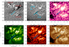 |
Fig. 1. Overview of the filament in a nest of three active regions. The northern filament (Nfil) does not evolve while the southern filament (Sfil) erupts, i.e., mainly its eastern part, which is marked with cyan contours in all the panels. The images were obtained by SDO/HMI, SDO/AIA, GONG, SUTRI, and STEREO/EUVI-A on 2022 October 4 before eruption. The filament is visible from the chromosphere to the transition region and the corona as a dark channel. The magnetogram shows that the filament lies in a mixed-polarity area between AR 13115 and AR 13114 (panel a) and extends along 350 arcsec in longitude (panel b). |
Observed information regarding the major activities of the eruption.
In the multiwavelength online movies provided by AIA, we see that the filament initially erupts in the northeast direction, and then goes through some process that causes it to erupt towards the southwest. The filament begins to lift up, as can be observed in all the EUV wavelengths around 13:25 UT. As the filament rises, two bright flare ribbons appear below it. These two bright ribbons are nearly parallel and gradually move away from each other with time, on both sides of the PIL. It is worth noting that one of the flare ribbons expands northward along a circular trajectory and shows a remote brightening at the end (see Fig. 2); this flare ribbon extends to the south of the active region AR 13117. The post-flare loops are also visible in the EUV bands. All of these activities may be the result of magnetic reconnection.
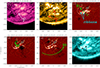 |
Fig. 2. Evolution of the filament eruption in multiple wavelengths between 13:30 UT and 15:20 UT. The filament rises up (white and red arrows in panels a and b). Two flare ribbons are highly visible in difference images in AIA 304 Å (14:00−14:40−15:20 minus 12:00 UT) (panels c–e). Cyan and black arrows stand for flare ribbons and post-flare loops in panels c and f, respectively. At 14:00 UT, the south ribbon is extended and turns to the north, creating a remote brightening. At its end, a remote dimming appears at 14:00 UT in S2 during the eruption. Three slices, labeled S1, S2, and S3, along the direction of filament eruption (initial stage), the dimming region propagation, and filament deflection are indicated by green arrows (panels c–e). S1 is along the straight arrow, and S2 and S3 are the arc slices. These slices are used for the time–distance analysis in Figs. 3 and 4. |
The filament keeps rising in a northeast direction and begins to erupt around 14:00 UT (see white and red arrows in Fig. 2). From the large field of view of the 304 Å images shown in Fig. 2, the eruption can be clearly divided into two stages. In the first stage, the direction of elevation is northeast. The nonradial direction of the filament’s initial eruption is also noteworthy. However, as the filament reaches a certain height, in the second stage, the direction is distinctly different from that of the previous stage. The direction of the eruption is now southwest. We would like to know what causes this deflection in direction. The entire eruption process is shown in Fig. 2 and the positions of several slices are plotted on it. A slice diagram of the filament eruption is shown in Fig. 3.
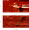 |
Fig. 3. Time–distance diagrams of the filament in AIA 304 Å for two stages. The diagrams show the rising and initial eruption of the filament along S1 (top panel) and subsequent deflection (bottom panel) along S3. The positions of flare ribbons are marked by cyan arrows. |
The slice diagram in panel a of Fig. 3 shows an obvious change in the direction of the filament during the eruption. S1 is a line slice along the direction of filament eruption (initial stage), S2 and S3 are arc slices along the dimming region propagation and filament deflection, respectively. Along the direction of S1, the filament rises slowly at first and then accelerates, and its velocity after deflection is followed by a speed of 101 km s−1. This diagram demonstrates the sweeping motion of the filament in a southwestern direction along S3 with a speed of 123 km s−1.
During the eruption, coronal dimming is observed in the northeast and propagates anticlockwise in the EUV bands. Meanwhile, we also observe a bright flare ribbon extending to the dimming area. There is a temporal correlation between the dimming region and the subsequent deflection. Figure 4 shows time–distance diagrams of four EUV bands along S2, which is the direction in which the dimming area propagates. The remote brightening and remote dimming region (S2) are represented by black and white arrows, respectively. The dimming comes after the remote brightening, with a delay of about 25 min. As the dimming propagates, a continuous brightening appears in front of it in the 304 Å images.
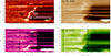 |
Fig. 4. Time–distance diagrams of the dimming region in EUV bands of S2. Black and white arrows represent the remote brightening (labeled “RB”) and remote dimming region (S2), respectively. |
In the online movie of 193 Å, the ends of two parallel flare ribbons bend into hook shapes – marked by yellow ovals in Fig. 5 – during the eruption, where the twin dimming occurs. The areas of the hooks shrink gradually with time, similarly to the process described by Aulanier & Dudík (2019). The twin dimming corresponds to the two footpoints of the magnetic flux rope that subsequently erupts. We selected the twin dimming locations, which we denote LD and RD (white boxes in Fig. 5 panel a), and calculated the magnetic flux for the two individual dimmings, as shown in panels b and c of Fig. 5. These two dimming regions correspond to the two footpoints of the filament. The left side of the filament is rooted in negative polarity, and the negative magnetic flux at the left footpoint gradually decreases, while the positive flux increases before the eruption. For the right footpoint, it is rooted in positive polarity. Positive flux first increases and then decreases for a period of time, while negative flux decreases by a small amount before the eruption but increases after the eruption. This indicates that magnetic emergence and magnetic cancelation occur at both footpoints before the eruption of the filament. Magnetic activities at the footpoints make the filament increasingly unstable, setting the stage for the subsequent eruption. During the eruption, the two ribbons move away from each other, and as the filament changes direction, the left leg of the flux rope approaches the coronal hole (indicated as CH marked in white in panel a of Fig. 5). The filament field lines could interact with the open field lines of the CH according to the online (movie_bd.mp4).
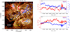 |
Fig. 5. Evolution of magnetic flux at two filament footpoints. The 193 Å image is overlaid with the longitudinal magnetic field. Red and blue contours indicate the magnetic field Bz at −50 G and 50 G, respectively. The white boxes represent the areas where the flux is calculated. The evolution of the left dimming (LD) flux is shown in panel b while the right dimming (RD) is shown in panel c. CH (written in white) represents the coronal hole. Yellow ellipses and arrows indicate the hooks at the ends of the flare ribbons. |
We obtained the radio dynamic spectra associated with this filament eruption from observations by HUMAIN1 of the Royal Observatory of Belgium, which is part of the network of Compound Astronomical Low frequency Low cost Instrument for Spectroscopy and Transportable Observatory (CALLISTO). There is a type III radio burst around 14:10 UT shown in Fig. 6, which indicates the interaction with open field lines, which could correspond to the coronal hole.
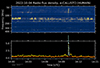 |
Fig. 6. Radio dynamic spectra from CALLISTO, exhibiting a Type III radio burst (cyan peak). |
During the filament eruption, a halo CME was observed by the Large Angle Spectrometric Coronagraph (LASCO; Brueckner et al. 1995) on board SOHO (Domingo et al. 1995). The CME started at 14:12:05 UT with a linear fit velocity of 926 km s−1 (see green arrows in Fig. 7) provided by the SOHO LASCO CME catalog2. The direction of the CME is roughly radial. In the online movie, the CME shows close correspondence with the eruption.
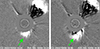 |
Fig. 7. Coronal mass ejections observed by LASCO. The CME to the south is correlated with the filament eruption marked by a green arrow. The north–west CME is ejected at 13:25 UT from another AR located close to the western limb (AR 13113). |
4. Three-dimensional magnetic field modeling
To investigate potential reconnection geometries during the eruption, we reconstructed 3D coronal magnetic fields involved in the filament eruption. Nonlinear force-free-field (NLFFF) extrapolation – concentrating on the magnetic configuration of the active region – and polytropic global coronal MHD modeling are adopted in this paper. Importantly, we note that it is the typical magnetic topology that is responsible for magnetic reconnection processes taking place in the low and high corona.
The NLFFF extrapolation is achieved using the magneto-friction relaxation module in the MPI-AMRVAC framework (Guo et al. 2016a,b; Xia et al. 2018). In this model, the magnetic field is totally dominated by the magnetic-induced equation with a velocity nearly proportional to the local Lorentz force, such that the converged state approaches a force-free state. The implementation of the NLFFF extrapolation includes the preprocessing for the bottom boundary condition and computation of coronal magnetic fields, as follows.
First, we carried out pre-processing of the input magnetograms, which serve as the bottom boundary condition of the extrapolation. We corrected the projection effects and removed the Lorentz force and torque using the method of Wiegelmann et al. (2006) so as to conform to the force-free assumption. This approach entails an optimization method to minimize the function composed of four terms (Eq. (6) in Wiegelmann et al. 2006), including the deviation from the observational data, smoothness of the magnetic fields, and the Lorentz force and torque. By taking this approach, the Lorentz force and torque can be reduced to a small value, resulting in a smooth vector magnetic field within the measurement error. We performed 5000 iterations for each magnetogram, after which the Lorentz force and torque decreased to one-thousandth of the original magnitudes (quantified by ϵforce and ϵtorque in Wiegelmann et al. 2006). We can state that the forces are nearly null and the magnetic configuration is almost stable. Subsequently, we reconstructed the 3D coronal magnetic fields. As shown in the observations, the eruptive filament is located at the edge of the active region, which can be categorized as intermediate type. In this case, it was difficult to construct the sheared and twisted magnetic fields of the filament for two reasons. On the one hand, the vector magnetic fields in decayed regions are highly noisy in general. On the other hand, the intermediate filament is generally high-lying, meaning that the information is harder to transform precisely from the input photosphere magnetograms to the positions of the filament due to the errors during the numerical computation. To this end, following the method of our previous works (Guo et al. 2019, 2021b), we embedded a twisted flux rope with the regularized Biot-Savart Laws (RBSL) method into the potential field, in which the axis of the inserted flux rope is parallel to the path of the filament in observations. Next, we relaxed the aforementioned magnetic fields to a force-free state with the magneto-frictional model. After 60 000 iterations, the force-free and divergence metrics are 0.35 and 3.55 × 10⁻⁵, respectively. Compared to our previous studies, the values of these two metrics are acceptable.
Figure 8 shows the results of the NLFFF extrapolation, which are overlaid on the viewing angle of AIA observations. The green, pink, and dark cyan tubes represent the magnetic structures of the eruptive filament, the fan-spine structure, and the peripheral active regions, respectively. Based on the alignment between the typical field lines and flare ribbons, we conclude that two parallel and circular flare ribbons are formed due to magnetic reconnection in overlying arcades and the fan-spine reconnection. Additionally, we also find that the dimming is surrounded by circular ribbons (Fig. 2), which may suggest an interchange magnetic reconnection is taking place, which could be causing the jump and expansion of the flux rope footpoint. In conclusion, the NLFFF extrapolation at the scale of the active region explains many physical processes seen in observations, and in particular the circular ribbons and dimmings. The inserted flux rope visualized in Fig. 8 represents the filament before its eruption and subsequent change of direction. The inserted RBSL flux rope represents an extended filament adopting the global magnetohydrodynamic (MHD) modeling. The global view of the ribbons in Fig. 2 corresponds to this configuration. It is clear that the remote circular brightening and dimming, labeled S2 in Fig. 2, corresponds to this complex nest of active regions in a multipolar configuration. The remote circular brightening and dimming could be related to footpoints of arcades corresponding to the fan-spine. A data-driven analysis should be performed to clearly understand the process of rotation and deflection of the filament before the ejection of the CME.
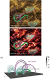 |
Fig. 8. Magnetic configuration of the three ARs (13114, 13115, 13117) and the intermediate filament before activity provided by a NLFFF magnetic field extrapolation using a magneto-frictional model. Panels a and b show magnetic field lines presented from the perspective of AIA observations, and panel c shows these in a 3D view. The green twisted field lines represent the regularized Biot-Savart flux rope (eruptive filament) inserted in the magnetic extrapolated configuration, the dark cyan lines represent the overlying arcades in the AR and its surroundings, and the pink lines represent the fan and the spine over the filament. |
The Type III radio burst (Fig. 6) indicates an interchange reconnection with the open field lines. To verify the existence of open field lines, we performed a global MHD modeling including the solar wind using the model COCONUT (Perri et al. 2022). Based on this global MHD modeling, we were able to investigate the magnetic structures near this active region. This modeling includes the following steps: First, the initial magnetic fields are provided by the potential-field source-surface (PFSS) model computed with a fast finite-volume solver in COCONUT (Perri et al. 2022). The bottom input magenetogram is preprocessed with the spherical harmonics projection with a maximum frequency of lmax = 30. Hereafter, we relax the above state with the polytropic MHD model. After 35 700 relaxation steps, a convergence level of 10−5 is reached, meaning that the quasi-static solar-wind solution has been attained (see Guo et al. 2024).
Figure 9 shows the typical field lines in the global coronal modeling. One can see fan-spine structure (green tubes), overlying closed arcades (purple tubes), and the open field lines (yellow tubes) toward the south, corresponding to the coronal hole (panel a). We posit that the magnetic reconnection between the eruptive flux rope and the open fields can inject energetic particles into the interplanetary space, driving a type III radio burst.
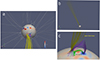 |
Fig. 9. Global coronal modeling with COCONUT of the AR environment, showing the reconnection with open field lines in the region of the dimming. The fan-spine structure (green tubes), overlying closed arcades (purple tubes), and the open field lines (yellow tubes) are presented. Panels b and c have been rotated by 180° to show the open field lines. |
5. Discussion and conclusions
In this paper, we present a detailed analysis of a filament eruption observed by SDO, STEREO, SUTRI, and GONG simultaneously. There are two stages to the filament eruption: in the first, the filament rises up toward the northeast, and in the second, the direction of the eruption is deflected toward the southwest, at which point the eruption can be considered nonradial.
Based on the combination of simultaneous observations from multiple instruments, NLFFF extrapolation, and a polytropic global MHD modeling, we propose the following scenario: In the beginning, the filament is initially restrained below a dome of a fan-spine configuration (shown by the pink lines in Fig. 8). Due to the continuous magnetic activities at the footpoints, the filament gradually begins to rise toward the northeast. According to Aulanier & Dudík (2019), it is possible to define the geometry of three types of 3D magnetic reconnections, namely “aa-rf” reconnection, “ar-rf” reconnection, and “rr-rf” reconnection. In our case, it is possible we are seeing an aa-rf magnetic reconnection above the filament, resulting in two bright flare ribbons and post-flare loops. Such reconnection can disassemble the restraint above the filament and drive the filament to keep rising, which sets the stage for the magnetic reconnection later on. One of the flare ribbons expands along a circular trajectory. When the filament reaches a certain height, it reconnects with the open field lines besides it (yellow lines in Fig. 9). Plasma is accelerated at the reconnection point and propagates outward along the open magnetic lines, and so the plasma density decreases and the region darkens. After the reconnection, some new loops form. It is worth noting that the direction of the filament later in eruption is guided by the open magnetic field lines to the east. The direction of its deflection is the same as the direction in which the open magnetic field lines bend (Yang et al. 2015, 2018). This corresponds to subsequent observations of the CME.
This example provides evidence for the multiple magnetic reconnections experienced by large-scale filaments during eruption. Both the background magnetic field and the filament fibrils and strands contribute during magnetic reconnection. The findings presented here providing a new understanding of the diverse magnetic fields and energy exchanges of solar eruptive activity. We look forward to developing more high-resolution instruments in the future and using high-resolution data to study the filament-eruption process in as much detail as possible.
Movies
Movie 1 (movie_bd) Access Supplementary Material
Movie 2 (all) Access Supplementary Material
Movie 3 (GONG_Ha) Access Supplementary Material
Acknowledgments
We thank the referee for careful reading and many constructive comments. This work is supported by the NSFC grant 12173022, 11790303 and 11973031. The authors are indebted to the SDO, STEREO, SUTRI, GONG, SOHO and CALLISTO teams for providing the data. We are very grateful to Zhang Liang for his help in data processing. SUTRI is a collaborative project conducted by the National Astronomical Observatories of CAS, Peking University, Tongji University, Xi’an Institute of Optics and Precision Mechanics of CAS and the Innovation Academy for Microsatellites of CAS. Data were acquired by GONG instruments operated by NISP/NSO/AURA/NSF with contribution from NOAA. SOHO is a project of international cooperation between ESA and NASA.
References
- Alexander, C. E., Walsh, R. W., Régnier, S., et al. 2013, ApJ, 775, L32 [NASA ADS] [CrossRef] [Google Scholar]
- Attrill, G., Nakwacki, M. S., Harra, L. K., et al. 2006, Sol. Phys., 238, 117 [Google Scholar]
- Aulanier, G., & Dudík, J. 2019, A&A, 621, A72 [NASA ADS] [CrossRef] [EDP Sciences] [Google Scholar]
- Babcock, H. W., & Babcock, H. D. 1955, ApJ, 121, 349 [Google Scholar]
- Bai, X., Tian, H., Deng, Y., et al. 2023, Res. Astron. Astrophys., 23, 065014 [CrossRef] [Google Scholar]
- Bi, Y., Jiang, Y. C., Yang, L. H., & Zheng, R. S. 2011, New Astron., 16, 276 [NASA ADS] [CrossRef] [Google Scholar]
- Bi, Y., Jiang, Y., Yang, J., et al. 2013, ApJ, 773, 162 [NASA ADS] [CrossRef] [Google Scholar]
- Bi, Y., Jiang, Y., Yang, J., et al. 2015, ApJ, 805, 48 [NASA ADS] [CrossRef] [Google Scholar]
- Brueckner, G. E., Howard, R. A., Koomen, M. J., et al. 1995, Sol. Phys., 162, 357 [NASA ADS] [CrossRef] [Google Scholar]
- Chandra, R., Démoulin, P., Devi, P., Joshi, R., & Schmieder, B. 2021, ApJ, 922, 227 [NASA ADS] [CrossRef] [Google Scholar]
- Chen, P. F., Harra, L. K., & Fang, C. 2014, ApJ, 784, 50 [NASA ADS] [CrossRef] [Google Scholar]
- Chen, H., Duan, Y., Yang, J., Yang, B., & Dai, J. 2018, ApJ, 869, 78 [CrossRef] [Google Scholar]
- Cheng, J. X., & Qiu, J. 2016, ApJ, 825, 37 [NASA ADS] [CrossRef] [Google Scholar]
- Cheng, X., Kliem, B., & Ding, M. D. 2018, ApJ, 856, 48 [Google Scholar]
- Dai, J., Li, Z., Wang, Y., et al. 2022, ApJ, 929, 85 [NASA ADS] [CrossRef] [Google Scholar]
- Deng, Y., Lin, Y., Schmieder, B., & Engvold, O. 2002, Sol. Phys., 209, 153 [NASA ADS] [CrossRef] [Google Scholar]
- Domingo, V., Fleck, B., & Poland, A. I. 1995, Sol. Phys., 162, 1 [Google Scholar]
- Gibson, S. E., Fan, Y., Török, T., & Kliem, B. 2006, Space Sci. Rev., 124, 131 [Google Scholar]
- Gilbert, H., Kilper, G., & Alexander, D. 2007, ApJ, 671, 978 [Google Scholar]
- Gold, T., & Hoyle, F. 1960, MNRAS, 120, 89 [NASA ADS] [Google Scholar]
- Gopalswamy, N., Yashiro, S., Krucker, S., Stenborg, G., & Howard, R. A. 2004, J. Geophys. Res.: Space Phys., 109, A12105 [NASA ADS] [CrossRef] [Google Scholar]
- Gopalswamy, N., Mäkelä, P., Xie, H., Akiyama, S., & Yashiro, S. 2009, J. Geophys. Res.: Space Phys., 114, A00A22 [Google Scholar]
- Gui, B., Shen, C., Wang, Y., et al. 2011, Sol. Phys., 271, 111 [NASA ADS] [CrossRef] [Google Scholar]
- Guo, Y., Xia, C., & Keppens, R. 2016a, ApJ, 828, 83 [NASA ADS] [CrossRef] [Google Scholar]
- Guo, Y., Xia, C., Keppens, R., & Valori, G. 2016b, ApJ, 828, 82 [NASA ADS] [CrossRef] [Google Scholar]
- Guo, Y., Xu, Y., Ding, M. D., et al. 2019, ApJ, 884, L1 [NASA ADS] [CrossRef] [Google Scholar]
- Guo, Y., Hou, Y., Li, T., & Zhang, J. 2021a, ApJ, 920, 77 [NASA ADS] [CrossRef] [Google Scholar]
- Guo, J. H., Ni, Y. W., Qiu, Y., et al. 2021b, ApJ, 917, 81 [NASA ADS] [CrossRef] [Google Scholar]
- Guo, J. H., Qiu, Y., Ni, Y. W., et al. 2023, ApJ, 956, 119 [NASA ADS] [CrossRef] [Google Scholar]
- Guo, J. H., Linan, L., Poedts, S., et al. 2024, A&A, 683, A54 [NASA ADS] [CrossRef] [EDP Sciences] [Google Scholar]
- Harvey, J. W., Hill, F., Hubbard, R. P., et al. 1996, Science, 272, 1284 [Google Scholar]
- Hood, A. W., & Priest, E. R. 1981, Geophys. Astrophys. Fluid Dyn., 17, 297 [NASA ADS] [CrossRef] [Google Scholar]
- Hou, Y., Li, T., Yang, S., & Zhang, J. 2019, ApJ, 871, 4 [Google Scholar]
- Hou, Y., Li, C., Li, T., et al. 2023, ApJ, 959, 69 [NASA ADS] [CrossRef] [Google Scholar]
- Hu, H., Liu, Y. D., Chitta, L. P., Peter, H., & Ding, M. 2022, ApJ, 940, L12 [NASA ADS] [CrossRef] [Google Scholar]
- Jiang, Y., Ji, H., Wang, H., & Chen, H. 2003, ApJ, 597, L161 [NASA ADS] [CrossRef] [Google Scholar]
- Jiang, Y., Yang, L., Li, K., & Shen, Y. 2007, ApJ, 667, L105 [NASA ADS] [CrossRef] [Google Scholar]
- Jin, M., Cheung, M. C. M., DeRosa, M. L., Nitta, N. V., & Schrijver, C. J. 2022, ApJ, 928, 154 [NASA ADS] [CrossRef] [Google Scholar]
- Joshi, N. C., Srivastava, A. K., Filippov, B., et al. 2014, ApJ, 787, 11 [NASA ADS] [CrossRef] [Google Scholar]
- Joshi, R., Mandrini, C. H., Chandra, R., et al. 2022, Sol. Phys., 297, 81 [NASA ADS] [CrossRef] [Google Scholar]
- Kaiser, M. L., Kucera, T. A., Davila, J. M., et al. 2008, Space Sci. Rev., 136, 5 [Google Scholar]
- Kliem, B., & Török, T. 2006, Phys. Rev. Lett., 96, 255002 [Google Scholar]
- Koleva, K., Devi, P., Chandra, R., et al. 2022, Sol. Phys., 297, 44 [NASA ADS] [CrossRef] [Google Scholar]
- Kumar, P., Srivastava, A. K., Filippov, B., Erdélyi, R., & Uddin, W. 2011, Sol. Phys., 272, 301 [NASA ADS] [CrossRef] [Google Scholar]
- Kumar, P., Karpen, J. T., Antiochos, S. K., et al. 2023, ApJ, 943, 156 [NASA ADS] [CrossRef] [Google Scholar]
- Lemen, J. R., Title, A. M., Akin, D. J., et al. 2012, Sol. Phys., 275, 17 [Google Scholar]
- Li, T., Yang, S., Zhang, Q., Hou, Y., & Zhang, J. 2018, ApJ, 859, 122 [Google Scholar]
- Li, Z. F., Cheng, X., Ding, M. D., et al. 2023, A&A, 673, A83 [NASA ADS] [CrossRef] [EDP Sciences] [Google Scholar]
- Liu, Y., Su, J., Xu, Z., et al. 2009, ApJ, 696, L70 [NASA ADS] [CrossRef] [Google Scholar]
- Low, B. C. 1990, ARA&A, 28, 491 [NASA ADS] [CrossRef] [Google Scholar]
- Martin, S. F. 1986, NASA Conf. Publ., 2442, 73 [Google Scholar]
- Monga, A., Sharma, R., Liu, J., et al. 2021, MNRAS, 500, 684 [Google Scholar]
- Perri, B., Leitner, P., Brchnelova, M., et al. 2022, ApJ, 936, 19 [NASA ADS] [CrossRef] [Google Scholar]
- Pesnell, W. D., Thompson, B. J., & Chamberlin, P. C. 2012, Sol. Phys., 275, 3 [Google Scholar]
- Reinard, A. A., & Biesecker, D. A. 2008, ApJ, 674, 576 [NASA ADS] [CrossRef] [Google Scholar]
- Ruan, G., Chen, Y., Wang, S., et al. 2014, ApJ, 784, 165 [NASA ADS] [CrossRef] [Google Scholar]
- Ruan, G., Chen, Y., & Wang, H. 2015, ApJ, 812, 120 [NASA ADS] [CrossRef] [Google Scholar]
- Ruan, G., Schmieder, B., Mein, P., et al. 2018, ApJ, 865, 123 [NASA ADS] [CrossRef] [Google Scholar]
- Ruan, G., Jejčič, S., Schmieder, B., et al. 2019a, ApJ, 886, 134 [NASA ADS] [CrossRef] [Google Scholar]
- Ruan, G., Schmieder, B., Masson, S., et al. 2019b, ApJ, 883, 52 [NASA ADS] [CrossRef] [Google Scholar]
- Sakai, J.-I., & Koide, S. 1992, Sol. Phys., 137, 293 [CrossRef] [Google Scholar]
- Schmieder, B., & Aulanier, G. 2012, Adv. Space Res., 49, 1598 [NASA ADS] [CrossRef] [Google Scholar]
- Schmieder, B., Démoulin, P., & Aulanier, G. 2013, Adv. Space Res., 51, 1967 [Google Scholar]
- Schmieder, B., Cremades, H., Mandrini, C., Démoulin, P., & Guo, Y. 2014, in Nature of Prominences and their Role in Space Weather, eds. B. Schmieder, J. M. Malherbe, & S. T. Wu, 300, 489 [NASA ADS] [Google Scholar]
- Schmieder, B., Zuccarello, F. P., Aulanier, G., et al. 2016, Cent. Eur. Astrophys. Bull., 40, 35 [Google Scholar]
- Schou, J., Scherrer, P. H., Bush, R. I., et al. 2012, Sol. Phys., 275, 229 [Google Scholar]
- Schrijver, C. J., Elmore, C., Kliem, B., Török, T., & Title, A. M. 2008, ApJ, 674, 586 [NASA ADS] [CrossRef] [Google Scholar]
- Shen, Y.-D., Liu, Y., & Liu, R. 2011a, Res. Astron. Astrophys., 11, 594 [CrossRef] [Google Scholar]
- Shen, C., Wang, Y., Gui, B., Ye, P., & Wang, S. 2011b, Sol. Phys., 269, 389 [NASA ADS] [CrossRef] [Google Scholar]
- Shen, Y., Liu, Y., & Su, J. 2012, ApJ, 750, 12 [NASA ADS] [CrossRef] [Google Scholar]
- Song, Y. L., Guo, Y., Tian, H., et al. 2018, ApJ, 854, 64 [NASA ADS] [CrossRef] [Google Scholar]
- Sterling, A. C., & Hudson, H. S. 1997, ApJ, 491, L55 [Google Scholar]
- Su, J., Liu, Y., Kurokawa, H., et al. 2007, Sol. Phys., 242, 53 [NASA ADS] [CrossRef] [Google Scholar]
- Sun, Z., Li, T., Tian, H., et al. 2023, ApJ, 953, 148 [CrossRef] [Google Scholar]
- Tian, H., McIntosh, S. W., Xia, L., He, J., & Wang, X. 2012, ApJ, 748, 106 [NASA ADS] [CrossRef] [Google Scholar]
- Tripathi, D., Gibson, S. E., Qiu, J., et al. 2009, A&A, 498, 295 [NASA ADS] [CrossRef] [EDP Sciences] [Google Scholar]
- Wiegelmann, T., Inhester, B., & Sakurai, T. 2006, Sol. Phys., 233, 215 [Google Scholar]
- Wuelser, J. P., Lemen, J. R., Tarbell, T. D., et al. 2004, in Telescopes and Instrumentation for Solar Astrophysics, eds. S. Fineschi, & M. A. Gummin, SPIE Conf. Ser., 5171, 111 [NASA ADS] [CrossRef] [Google Scholar]
- Xia, C., Teunissen, J., El Mellah, I., Chané, E., & Keppens, R. 2018, ApJS, 234, 30 [Google Scholar]
- Xu, H., Su, J., Chen, J., et al. 2020, ApJ, 901, 121 [NASA ADS] [CrossRef] [Google Scholar]
- Xue, Z., Yan, X., Wang, J., et al. 2023, ApJ, 945, 5 [NASA ADS] [CrossRef] [Google Scholar]
- Yan, X., Xue, Z., Cheng, X., et al. 2020, ApJ, 889, 106 [NASA ADS] [CrossRef] [Google Scholar]
- Yang, J., Jiang, Y., Xu, Z., Bi, Y., & Hong, J. 2015, ApJ, 803, 68 [NASA ADS] [CrossRef] [Google Scholar]
- Yang, J., Dai, J., Chen, H., Li, H., & Jiang, Y. 2018, ApJ, 862, 86 [CrossRef] [Google Scholar]
- Yang, J., Hong, J., Yang, B., Bi, Y., & Xu, Z. 2023a, ApJ, 942, 86 [NASA ADS] [CrossRef] [Google Scholar]
- Yang, L., Yan, X., Xue, Z., et al. 2023b, ApJ, 943, 62 [NASA ADS] [CrossRef] [Google Scholar]
- Zarro, D. M., Sterling, A. C., Thompson, B. J., Hudson, H. S., & Nitta, N. 1999, ApJ, 520, L139 [NASA ADS] [CrossRef] [Google Scholar]
- Zhang, Q. M. 2020, A&A, 642, A159 [NASA ADS] [CrossRef] [EDP Sciences] [Google Scholar]
- Zhang, Y., Zhang, Q., Dai, J., Li, D., & Ji, H. 2022a, Sol. Phys., 297, 138 [NASA ADS] [CrossRef] [Google Scholar]
- Zhang, Y., Yan, X., Wang, J., et al. 2022b, ApJ, 933, 200 [NASA ADS] [CrossRef] [Google Scholar]
- Zheng, R., Chen, Y., Wang, B., Li, G., & Xiang, Y. 2017, ApJ, 840, 3 [NASA ADS] [CrossRef] [Google Scholar]
- Zheng, R., Yang, S., Rao, C., et al. 2019, ApJ, 875, 71 [NASA ADS] [CrossRef] [Google Scholar]
- Zhou, C., Shen, Y., Zhou, X., et al. 2021, ApJ, 923, 45 [NASA ADS] [CrossRef] [Google Scholar]
- Zirker, J. B. 1989, Sol. Phys., 119, 341 [NASA ADS] [CrossRef] [Google Scholar]
- Zirker, J. B., Engvold, O., & Martin, S. F. 1998, Nature, 396, 440 [Google Scholar]
All Tables
All Figures
|
Fig. 1. Overview of the filament in a nest of three active regions. The northern filament (Nfil) does not evolve while the southern filament (Sfil) erupts, i.e., mainly its eastern part, which is marked with cyan contours in all the panels. The images were obtained by SDO/HMI, SDO/AIA, GONG, SUTRI, and STEREO/EUVI-A on 2022 October 4 before eruption. The filament is visible from the chromosphere to the transition region and the corona as a dark channel. The magnetogram shows that the filament lies in a mixed-polarity area between AR 13115 and AR 13114 (panel a) and extends along 350 arcsec in longitude (panel b). |
| In the text | |
|
Fig. 2. Evolution of the filament eruption in multiple wavelengths between 13:30 UT and 15:20 UT. The filament rises up (white and red arrows in panels a and b). Two flare ribbons are highly visible in difference images in AIA 304 Å (14:00−14:40−15:20 minus 12:00 UT) (panels c–e). Cyan and black arrows stand for flare ribbons and post-flare loops in panels c and f, respectively. At 14:00 UT, the south ribbon is extended and turns to the north, creating a remote brightening. At its end, a remote dimming appears at 14:00 UT in S2 during the eruption. Three slices, labeled S1, S2, and S3, along the direction of filament eruption (initial stage), the dimming region propagation, and filament deflection are indicated by green arrows (panels c–e). S1 is along the straight arrow, and S2 and S3 are the arc slices. These slices are used for the time–distance analysis in Figs. 3 and 4. |
| In the text | |
|
Fig. 3. Time–distance diagrams of the filament in AIA 304 Å for two stages. The diagrams show the rising and initial eruption of the filament along S1 (top panel) and subsequent deflection (bottom panel) along S3. The positions of flare ribbons are marked by cyan arrows. |
| In the text | |
|
Fig. 4. Time–distance diagrams of the dimming region in EUV bands of S2. Black and white arrows represent the remote brightening (labeled “RB”) and remote dimming region (S2), respectively. |
| In the text | |
|
Fig. 5. Evolution of magnetic flux at two filament footpoints. The 193 Å image is overlaid with the longitudinal magnetic field. Red and blue contours indicate the magnetic field Bz at −50 G and 50 G, respectively. The white boxes represent the areas where the flux is calculated. The evolution of the left dimming (LD) flux is shown in panel b while the right dimming (RD) is shown in panel c. CH (written in white) represents the coronal hole. Yellow ellipses and arrows indicate the hooks at the ends of the flare ribbons. |
| In the text | |
|
Fig. 6. Radio dynamic spectra from CALLISTO, exhibiting a Type III radio burst (cyan peak). |
| In the text | |
|
Fig. 7. Coronal mass ejections observed by LASCO. The CME to the south is correlated with the filament eruption marked by a green arrow. The north–west CME is ejected at 13:25 UT from another AR located close to the western limb (AR 13113). |
| In the text | |
|
Fig. 8. Magnetic configuration of the three ARs (13114, 13115, 13117) and the intermediate filament before activity provided by a NLFFF magnetic field extrapolation using a magneto-frictional model. Panels a and b show magnetic field lines presented from the perspective of AIA observations, and panel c shows these in a 3D view. The green twisted field lines represent the regularized Biot-Savart flux rope (eruptive filament) inserted in the magnetic extrapolated configuration, the dark cyan lines represent the overlying arcades in the AR and its surroundings, and the pink lines represent the fan and the spine over the filament. |
| In the text | |
|
Fig. 9. Global coronal modeling with COCONUT of the AR environment, showing the reconnection with open field lines in the region of the dimming. The fan-spine structure (green tubes), overlying closed arcades (purple tubes), and the open field lines (yellow tubes) are presented. Panels b and c have been rotated by 180° to show the open field lines. |
| In the text | |
Current usage metrics show cumulative count of Article Views (full-text article views including HTML views, PDF and ePub downloads, according to the available data) and Abstracts Views on Vision4Press platform.
Data correspond to usage on the plateform after 2015. The current usage metrics is available 48-96 hours after online publication and is updated daily on week days.
Initial download of the metrics may take a while.