| Issue |
A&A
Volume 687, July 2024
|
|
|---|---|---|
| Article Number | A266 | |
| Number of page(s) | 19 | |
| Section | Celestial mechanics and astrometry | |
| DOI | https://doi.org/10.1051/0004-6361/202449463 | |
| Published online | 23 July 2024 | |
Resonant chains in triple-planet systems
1
School of Astronomy and Space Science, Nanjing University,
163 Xianlin Avenue,
Nanjing
210046,
PR
China
e-mail: This email address is being protected from spambots. You need JavaScript enabled to view it.
2
Key Laboratory of Modern Astronomy and Astrophysics in Ministry of Education, Nanjing University,
Nanjing
210046,
PR
China
3
Instituto de Astronomía Teórica y Experimental (IATE), Observatorio Astronómico (OAC), Universidad Nacional de Córdoba,
Laprida
854,
Córdoba,
Argentina
Received:
2
February
2024
Accepted:
8
May
2024
Abstract
Context. The mean motion resonance is the most important mechanism that may dominate the dynamics of a planetary system. In a multi-planetary system consisting of N ≥ 3 planets, the planets may form a resonant chain when the ratios of orbital periods of planets can be expressed as the ratios of small integers T1: T2: ⋯ : TN = k1: k2: ⋯ : kN. Due to the high degree of freedom, the motion in such systems could be complex and difficult to depict.
Aims. In this paper, we investigate the dynamics and possible formation of the resonant chain in a triple-planet system.
Methods. We defined the appropriate Hamiltonian for a three-planet resonant chain and numerically averaged it over the synodic period. The stable stationary solutions – apsidal corotational resonances (ACRs) – of this averaged system, corresponding to the local extrema of the Hamiltonian function, can be searched out numerically. The topology of the Hamiltonian around these ACRs reveals their stabilities. We further constructed the dynamical maps on different representative planes to study the dynamics around the stable ACRs, and we calculated the deviation (χ2) of the resonant angle in the evolution from the uniformly distributed values, by which we distinguished the behaviour of critical angles. Finally, the formation of the resonant chain via convergent planetary migration was simulated and the stable configurations associated with ACRs were verified.
Results. We find that the stable ACR families arising from circular orbits always exist for any resonant chain, and they may extend to a high eccentricity region. Around these ACR solutions, regular motion can be found, typically in two types of resonant configurations. One is characterised by libration of both the two-body resonant angles and the three-body Laplace resonant angle, and the other by libration of only two-body resonant angles. The three-body Laplace resonance does not seem to contribute to the stability of the resonant chain much. The resonant chain can be formed via convergent migration, and the resonant configuration evolves along the ACR families to eccentric orbits once the planets are captured into the chain. Ideally, our methods introduced in this paper can be applied to any resonant chain of any number of planets at any eccentricity.
Key words: celestial mechanics / planets and satellites: dynamical evolution and stability
© The Authors 2024
 Open Access article, published by EDP Sciences, under the terms of the Creative Commons Attribution License (https://creativecommons.org/licenses/by/4.0), which permits unrestricted use, distribution, and reproduction in any medium, provided the original work is properly cited.
This article is published in open access under the Subscribe to Open model. This email address is being protected from spambots. You need JavaScript enabled to view it. to support open access publication.
1 Introduction
Thousands of exo-planetary systems, over one-fourth of which are multi-planetary systems, have been detected. According to their orbital architectures, these multi-planetary systems are categorised into separable, compact, and resonant planetary systems. The separable (secular) systems are protected from a mutual collision and a close encounter by the low angular momentum deficit (AMD), that is, the AMD stability (Laskar & Petit 2017). The compact multi-planetary systems, however, even for those with circular orbits, are generally unstable. Petit et al. (2020) show how the slow chaotic diffusion due to the overlap of three-body resonances dominates the timescale leading to the instability for initially coplanar and circular orbits, and this type of mechanism reproduces the qualitative behaviour found in numerical simulations very well (Hussain & Tamayo 2020). The resonant systems, in which planets are found in mean motion resonance (MMR) with each other, are likely to be stable and of particular interest because they may bear important clues as to the formation and evolution of planetary systems. For the case of two planets in an MMR, the dynamics are well understood through the resonant periodic orbits (e.g. Voyatzis 2008; Voyatzis et al. 2009) and the apsidal corotational resonance (ACR) (e.g. Michtchenko et al. 2008). But the resonant structure could be much richer and complex in multi-planetary systems.
Except for the two-body MMR involving two planets and the hosting star, the three-body resonance (three planets are involved) also plays a role (e.g. Petit 2021; Cerioni et al. 2022). Particularly, a multi-planetary system with orbital periods of neighbouring planets librating at a sequence of near-integer ratios (2/1, 3/2, 4/3, etc.), often referred to as a resonant chain, is of great interest. The well-known examples include three planets of Kepler-51 in a 1:2:3 resonant chain (Masuda 2014), four planets in a 1:2:4:8 resonant chain in HR8799 (Goździewski & Migaszewski 2020) and a 1:2:5:7 resonant chain in K2-32 (Heller et al. 2019), five planets of TOI-178 in a 2:4:6:9:12 (Leleu et al. 2021) and a 4:6:9:12:18 resonant chain in Kepler-80 (MacDonald et al. 2021), and another five planets composing a resonant chain of 3:2 MMRs in K2-138 (Christiansen et al. 2018; Lopez et al. 2019). In these systems, in addition to the transit light curves, a transit-timing variation (TTV), and radial velocity data, the dynamics of the resonant chain have also been taken into account to improve the planetary parameters (mass, orbital period, etc.).
Plenty of numerical studies have been devoted to the formation history and dynamical stability of multi-planetary systems with planets locked in or close to a resonant chain. At the early stage of a planetary system’s formation, planets can be captured into a resonant chain through the convergent orbital migration. The tidal effect and the accretion of matter (increasing planetary mass) may influence the further evolution, driving the planetary system away from the nominal positions of resonances, and destabilising the resonant chain via the secondary resonance. The final surviving systems exhibit complex resonant structures involving in a two-body MMR, three-body MMR, resonant chain, secular resonance, etc. (e.g. MacDonald & Dawson 2018; Pichierri et al. 2019; Morrison et al. 2020; Pichierri & Morbidelli 2020; MacDonald et al. 2022; Wong & Lee 2024).
Due to the high degree of freedom, the analytical method is difficult to be applied to such systems. Delisle (2017) proposes an analytical model for any resonant chain and successfully predicts the resonant configuration of Kepler-223 (Mills et al. 2016). And recently, Antoniadou & Voyatzis (2022) extended the methodology for a pair of resonant exoplanets in coplanar orbits (Antoniadou & Voyatzis 2016; Antoniadou 2016) to the case of triple massive coplanar planets in a resonant chain (general four-body problem) and, particularly, computed the resonant periodic orbits for the Kepler-51 system. Based on the stable periodic orbits of the 1:2:3 resonant chain, they demonstrate three possible scenarios that can safeguard the Kepler-51 planetary system. The comprehensive study on the stable periodic orbits can provide an optimum deduction of orbital elements, in addition to the observational data fitting.
In this paper, we generalise the semi-analytical model for analysing the periodic orbits in the coplanar two-body MMR first developed by Michtchenko et al. (2006) to the case of the resonant chain. For the sake of explaining our methods clearly, we mainly use the 1:2:3 resonance chain in the Kepler-51 system as an example in our analyses. But we emphasise here that the methods and some conclusions presented in this paper are general and can be applied to any other resonant chains of three or even more planets. In fact, we also briefly show our analyses on some other resonant chains in the end of this paper.
The rest part of this paper is organised as follows. In Sec. 2, we revisit the definition of resonant periodic orbits and generalise the definition to arbitrary resonant chains. We introduce our semi-analytical Hamiltonian method and the determination of ACR in the resonant chain in Sec. 3. Then this methodology is applied to the case of the 1:2:3 resonant chain, and the periodic orbits, that are, ACRs are obtained. In Sec. 4, the orbital dynamics around the stable ACRs are investigated. We study how the orbital configuration of planets in a resonant chain can be achieved via convergent planetary migration in Sec. 5. Finally, we draw our conclusion in Sec. 6.
2 The model
2.1 Rotational frame and resonant periodic orbits
The motion of planets in a resonant chain is often described in a rotational frame. Consider three massive planets m1, m2, m3 from the inside out orbiting around the central star M on the same plane, with their orbital periods T1, T2, T3 satisfying the commensurable condition
![Mathematical equation: $\[T_1: T_2: T_3=k_1: k_2: k_3, ~~\text {with } k_1, k_2, k_3 \in \mathcal{Z} \text {. }\]$](/articles/aa/full_html/2024/07/aa49463-24/aa49463-24-eq1.png) (1)
(1)
Following Antoniadou & Voyatzis (2022), a non-inertial frame (GXY) is introduced as follows. Let G coincide with the mass centre of M and m1, the axis GX always points to m1 from M, and GY be perpendicular to GX. In this rotating frame, m1 and M are always on the GX axis, while m2 and m3 revolve about m1 with the relative frequencies of n2 − n1 and n3 − n1, where n1, n2, n3 are the mean motions of three planets. The relative frequencies satisfy the near-integer commensurability:
![Mathematical equation: $\[\frac{n_2-n_1}{n_3-n_1}=\frac{p}{q}, ~\text { with } p, q \in \mathcal{Z} \text {. }\]$](/articles/aa/full_html/2024/07/aa49463-24/aa49463-24-eq2.png) (2)
(2)
The period T of the system, during which m2 revolves p times while m3 revolves q times both around m1, can be easily derived as
![Mathematical equation: $\[T=\frac{T_1}{1-T_1 / T_2} p=\frac{T_1}{1-T_1 / T_3} q.\]$](/articles/aa/full_html/2024/07/aa49463-24/aa49463-24-eq3.png) (3)
(3)
In practice, such periodicity requires that the planets m1, m2, and m3 repeat their configuration after time T. Therefore, the period T should be related to the least common multiple (LCM) of T1, T2, T3, and this type of periodic condition can be rewritten in a more general form
![Mathematical equation: $\[T / T_i=\operatorname{LCM}\left(k_1, k_2, k_3\right) / k_i, ~\text { for } i=1,2,3.\]$](/articles/aa/full_html/2024/07/aa49463-24/aa49463-24-eq4.png) (4)
(4)
For the 1:2:3 resonant chain in the planetary system Kepler-51, Eq. (4) gives LCM(1, 2, 3) = 6, and T = 6T1 = 3T2 = 2T3, which is equivalent to p = 3, q = 4 and T = 6T1 (Antoniadou & Voyatzis 2022). The periodicity defined in Eq. (4) can be generalised to resonant chain of N (N > 3) planets (e.g. a four-planet resonant system Kepler-223 can be found in Appendix B) as
![Mathematical equation: $\[T / T_i=\operatorname{LCM}\left(k_1, k_2, \cdots, k_N\right) / k_i, ~\text { for } i=1,2, \cdots, N \text {. }\]$](/articles/aa/full_html/2024/07/aa49463-24/aa49463-24-eq5.png) (5)
(5)
These periodic orbits can be found in the exact (nominal) location of the MMRs. In addition, according to different orbital configurations, these periodic orbits can be divided into two groups, namely the symmetric periodic orbits and the asymmetric ones. A periodic orbit is symmetric with respect to the GX axis of the rotating frame if it remains invariant under the fundamental symmetry (Hénon 2003) ∑: (t, X, Y) → (−t, X, −Y)
![Mathematical equation: $\[\begin{aligned}& X_i(-t)=X_i(t), \qquad Y_i(-t)=-Y_i(t), \\& \dot{X}_i(-t)=-\dot{X}_i(t), \quad \dot{Y}_i(-t)=\dot{Y}_i(t), \qquad i=1,2,3. \\&\end{aligned}\]$](/articles/aa/full_html/2024/07/aa49463-24/aa49463-24-eq6.png) (6)
(6)
This indicates that all the two-body MMRs should take the symmetric configuration. Otherwise, if one of the symmetry condition breaks, i.e. Eq. (6) is not satisfied for any i, then the configuration is referred as asymmetric. The relationship between symmetric condition and the choice of the resonant angles can also be found in e.g. Voyatzis (2008).
2.2 Hamiltonian description
The Hamiltonian of the planar three-planet (from the inside out m1, m2, m3) system takes the form (see e.g. Laskar 1991)
![Mathematical equation: $\[\begin{aligned}\mathcal{H} & =\mathcal{H}_0+\mathcal{H}_1 \\\mathcal{H}_0 & =\sum_{i=1}^3\left(\frac{\boldsymbol{p}_i^2}{2 M}-\mathcal{G} \frac{M m_i}{\left|\boldsymbol{r}_i\right|}\right), \\\mathcal{H}_1 & =\sum_{1 \leq i<j \leq 3} \frac{\boldsymbol{p}_i \cdot \boldsymbol{p}_j}{M}-\frac{\mathcal{G} m_i m_j}{\left|\boldsymbol{r}_i-\boldsymbol{r}_j\right|},\end{aligned}\]$](/articles/aa/full_html/2024/07/aa49463-24/aa49463-24-eq7.png) (7)
(7)
where ![Mathematical equation: $\[\mathcal{G}\]$](/articles/aa/full_html/2024/07/aa49463-24/aa49463-24-eq8.png) is the gravitational constant, ri is the position vector of the i-th planet, and pi is the canonically conjugated momentum. The
is the gravitational constant, ri is the position vector of the i-th planet, and pi is the canonically conjugated momentum. The ![Mathematical equation: $\[\mathcal{H}\]$](/articles/aa/full_html/2024/07/aa49463-24/aa49463-24-eq9.png) 0 is the sum of Keplerian part of each planet, while
0 is the sum of Keplerian part of each planet, while ![Mathematical equation: $\[\mathcal{H}\]$](/articles/aa/full_html/2024/07/aa49463-24/aa49463-24-eq10.png) 1 describes the interaction between planets. The Poincaré canoncial variables in astrocentric coordinate are
1 describes the interaction between planets. The Poincaré canoncial variables in astrocentric coordinate are
![Mathematical equation: $\[\begin{cases}\Lambda_i=\beta_i \sqrt{\mu_i a_i}, & \lambda_i \\ \Gamma_i=\Lambda_i\left(1-\sqrt{1-e_i^2}\right), & \gamma_i=-\varpi_i,\end{cases}\]$](/articles/aa/full_html/2024/07/aa49463-24/aa49463-24-eq11.png) (8)
(8)
where μi = ![Mathematical equation: $\[\mathcal{G}\]$](/articles/aa/full_html/2024/07/aa49463-24/aa49463-24-eq12.png) (M + mi), βi = miM/(mi + M), and ai, ei, ϖi, λi are the semi-major axis, eccentricity, longitude of periastron and the mean longitude of the i-th planet mi, respectively. The action variable Λi is the circular angular momentum and Γi is often referred as the AMD (see e.g. Petit et al. 2017).
(M + mi), βi = miM/(mi + M), and ai, ei, ϖi, λi are the semi-major axis, eccentricity, longitude of periastron and the mean longitude of the i-th planet mi, respectively. The action variable Λi is the circular angular momentum and Γi is often referred as the AMD (see e.g. Petit et al. 2017).
For two planets mi, mj with mean motions ni, nj, we denote by kji/kij = ni/nj = Tj/Ti the relative period ratio, and qij = qji = |kji − kij| the order of the resonance, where kij and kji are integers. The two-body resonant angles θij, Δϖij are defined as
![Mathematical equation: $\[\theta_{i j}=k_{j i} \lambda_j-k_{i j} \lambda_i-\left(k_{j i}-k_{i j}\right) \varpi_i, \quad \Delta \varpi_{i j}=\varpi_i-\varpi_j.\]$](/articles/aa/full_html/2024/07/aa49463-24/aa49463-24-eq13.png) (9)
(9)
For planetary systems near MMRs, Delisle (2017) introduces the canonical resonant variables for arbitrary resonant chain (with any number of planets, in resonances of any degree). Particularly, the resonant variables of the 1:2:3 resonant chain are
![Mathematical equation: $\[\begin{cases}\sigma_1=3 \lambda_3-2 \lambda_2-\varpi_1, & \Gamma_1, \\ \sigma_2=3 \lambda_3-2 \lambda_2-\varpi_2, & \Gamma_2, \\ \sigma_3=3 \lambda_3-2 \lambda_2-\varpi_3, & \Gamma_3, \\ \varphi_0=3 \lambda_3-4 \lambda_2+\lambda_1, & L_0=\Lambda_1, \\ \varphi_G=3 \lambda_3-2 \lambda_2, & G=\sum_{i=1}^3\left(\Lambda_i-\Gamma_i,\right) \\ Q=Q_{23}=\lambda_2-\lambda_3, & J=6 \Lambda_1+3 \Lambda_2+2 \Lambda_3.\end{cases}\]$](/articles/aa/full_html/2024/07/aa49463-24/aa49463-24-eq14.png) (10)
(10)
The first three angles in Eq. (10) are resonant angles conjugated to each planet’s AMD, and φ0 is the angle of Laplace resonance (0-th) between three planets. Since φG does not appear explicitly in the Hamiltonian (see details e.g. in Delisle 2017), the corresponding conjugated momentum G is constant, implying the preservation of angular momentum. Thus, the problem is in fact of five degree-of-freedom (DoF). The last angle Q is the fast angle with respect to the first four resonant angles (σ1, σ2, σ3,φ0), thus it can be removed by numerical averaging (see e.g. Gauss-Legendre formula, Press et al. 1996). The averaging process guarantees that J is another constant, which is similar to the ‘spacing parameter’ in the planar two-body MMR. Moreover, the integral constant J in triple-planet resonant chain T1: T2: T3 = k1: k2: k3 can be rewritten in a more general form L (hereafter we refer L as the spacing parameter in a resonant chain)
![Mathematical equation: $\[L=\sum_{i=1}^3 \frac{\Lambda_i}{k_i}.\]$](/articles/aa/full_html/2024/07/aa49463-24/aa49463-24-eq15.png) (11)
(11)
For the k1: k2: k3 = 1: 2: 3 resonant chain, during the period T (see the definition in Eq. (4)), the angle Q evolves
![Mathematical equation: $\[Q^T=2 \pi \times \operatorname{LCM}\left(k_1, k_2, k_3\right)\left(\frac{1}{k_2}-\frac{1}{k_3}\right)=2 \pi.\]$](/articles/aa/full_html/2024/07/aa49463-24/aa49463-24-eq16.png) (12)
(12)
Therefore, the averaged Hamiltonian ![Mathematical equation: $\[\bar{\mathcal{H}}\]$](/articles/aa/full_html/2024/07/aa49463-24/aa49463-24-eq17.png) can be defined as
can be defined as
![Mathematical equation: $\[\bar{\mathcal{H}}=\frac{1}{Q^T} \int_0^{Q^T} \mathcal{H} \mathrm{d} Q.\]$](/articles/aa/full_html/2024/07/aa49463-24/aa49463-24-eq18.png) (13)
(13)
The resonant periodic orbits will appear as stationary solution of the averaged Hamiltonian Eq. (13). After the numerical averaging process, the final Hamiltonion ![Mathematical equation: $\[\bar{\mathcal{H}}\]$](/articles/aa/full_html/2024/07/aa49463-24/aa49463-24-eq19.png) is of 4 DoF in canonical variables (σ1, σ2, σ3, φ0, Γ1; Γ2, Γ3, L0) parametrised by the two constants (L, G).
is of 4 DoF in canonical variables (σ1, σ2, σ3, φ0, Γ1; Γ2, Γ3, L0) parametrised by the two constants (L, G).
Seemingly, the resonance between m2 and m3 plays an essential role in Eq. (10), but it is only due to the arbitrary choice of the canonical variables. For any different choice of resonant angles, the expression of the synodic angle Q would be different. For example, the choices Q = Q12 = λ1 − λ2, or Q = Q13 = λ1 − λ3, the averaged Hamiltonian should be respectively calculated by:
![Mathematical equation: $\[\begin{aligned}\bar{\mathcal{H}} & =\frac{1}{Q_{12}^T} \int_0^{Q_{12}^T} \mathcal{H} \mathrm{d} Q_{12}=\frac{1}{Q_{13}^T} \int_0^{Q_{13}^T} \mathcal{H} \mathrm{d} Q_{13}, \\Q_{12}^T & =2 \pi \times \operatorname{LCM}\left(k_1, k_2, k_3\right)\left(\frac{1}{k_1}-\frac{1}{k_2}\right)=6 \pi, \\Q_{13}^T & =2 \pi \times \operatorname{LCM}\left(k_1, k_2, k_3\right)\left(\frac{1}{k_1}-\frac{1}{k_3}\right)=8 \pi.\end{aligned}\]$](/articles/aa/full_html/2024/07/aa49463-24/aa49463-24-eq20.png) (14)
(14)
For a better characterisation of the resonant configuration, we perform the linear transformation to angular variables defined in Eq. (10), and the resonant angles (θ12, Δϖ12, θ23, Δϖ23) between consecutive planets can be obtained as:
![Mathematical equation: $\[\begin{cases}\theta_{12}=2 \lambda_2-\lambda_1-\varpi_1, & \Delta \varpi_{12}=\varpi_1-\varpi_2, \\ \theta_{23}=3 \lambda_3-2 \lambda_2-\varpi_2, & \Delta \varpi_{23}=\varpi_2-\varpi_3.\end{cases}\]$](/articles/aa/full_html/2024/07/aa49463-24/aa49463-24-eq21.png) (15)
(15)
The first two angles θ12, Δϖ12 are for the MMR between the inner two planets m1, m2 while θ23, Δϖ23 are for the outer planets m2, m3 respectively, just as defined in Eq. (9).
For isolated two-body MMRs, the resonant angles (θij, Δϖij) are all 2π-periodic, i.e., the geometric configuration of MMR characterised by (θij, Δϖij) is identical to the one by (θij + 2k′π,Δϖij + 2k″π), with k′,k″ ∈ ![Mathematical equation: $\[\mathcal{Z}\]$](/articles/aa/full_html/2024/07/aa49463-24/aa49463-24-eq22.png) . For the 1:2:3 resonant chain, the averaged Hamiltonian Eq. (13) is 2π-periodically dependent on all the angular variables defined in Eq. (15). According to the symmetry in the co-rotational frame GXY with respect to m1, the configuration, in which the resonant angles (θ12, Δϖ12, θ23, Δϖ23) take either 0 or π, is symmetric, while other configurations are asymmetric. It should be noted that the above conditions may not always guarantee the proper periodicity and symmetric configuration for a general three-planet resonant chain if we choose the resonant angles between adjacent planets (rather θi,i+1, Δϖi,i+1 than θi,i+2, Δϖi,i+2) to characterise the system. We leave a detailed discussion for this problem to Appendix A.
. For the 1:2:3 resonant chain, the averaged Hamiltonian Eq. (13) is 2π-periodically dependent on all the angular variables defined in Eq. (15). According to the symmetry in the co-rotational frame GXY with respect to m1, the configuration, in which the resonant angles (θ12, Δϖ12, θ23, Δϖ23) take either 0 or π, is symmetric, while other configurations are asymmetric. It should be noted that the above conditions may not always guarantee the proper periodicity and symmetric configuration for a general three-planet resonant chain if we choose the resonant angles between adjacent planets (rather θi,i+1, Δϖi,i+1 than θi,i+2, Δϖi,i+2) to characterise the system. We leave a detailed discussion for this problem to Appendix A.
We note that the aforementioned procedure can be simply extended to systems containing N (N > 3) planets, in which the two constants take the form:
![Mathematical equation: $\[\begin{aligned}G & =\sum_{i=1}^N \beta_i \sqrt{\mu_i a_i\left(1-e_i^2\right)}, \\L & =\sum_{i=1}^N \frac{\beta_i \sqrt{\mu_i a_i}}{k_i}.\end{aligned}\]$](/articles/aa/full_html/2024/07/aa49463-24/aa49463-24-eq23.png) (16)
(16)
And the resonant configuration for an N-planet system can be represented by (θ12, Δϖ12, ⋯, θn−1,n, Δϖn−1,n).
Now, searching for the resonant periodic orbits is equivalent to finding the stationary solution of the averaged Hamiltonian with two free constants L and G.
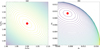 |
Fig. 1 Topology of the Hamiltonian on different representative planes, (a) The topology on period ratio plane (n1/n2, n2/n3) with fixed eccentricities. (b) The topology on eccentricity plane (e1,e2). The stationary solution located at (n1/n2, n2/n3) = (2, 1.5) and (e1, e2, e3) = (0.00458, 0.00938, 0.00564) is marked by a red dot on both panels. The corresponding critical angles are (θ12, Δϖ12, θ23, Δϖ23) = (π, 0, π, π). The colour indicates the value of Hamiltonian, light yellow for high and dark blue for low. The same colour code is adopted in all figures in this paper, unless otherwise stated. |
3 Topology of Hamiltonian and stationary solutions
The averaged Hamiltonian Eq. (13) has been reduced to 4 DoF. Due to the complex structure in high dimensional phase space (eight-dimensional phase space for aplanar three-planet system), searching for stationary solutions in the entire phase space is very difficult. Fortunately, the topology of the Hamiltonian ![Mathematical equation: $\[\bar{\mathcal{H}}\]$](/articles/aa/full_html/2024/07/aa49463-24/aa49463-24-eq24.png) can be understood from several representative planes (section of phase space), namely, the period ratio plane (n1/n2, n2/n3), the eccentricity plane (e1, e2) or (e2, e3), and the angular planes (θ12, Δϖ12) and (θ23, Δϖ23).
can be understood from several representative planes (section of phase space), namely, the period ratio plane (n1/n2, n2/n3), the eccentricity plane (e1, e2) or (e2, e3), and the angular planes (θ12, Δϖ12) and (θ23, Δϖ23).
Hereafter, as an example, we focus on a 1:2:3 resonant chain with the mass parameters of M = 1.0, m1 = 2.1 × 10⁻⁶, m2 = 4.0 × 10⁻⁶, m3 = 7.6 × 10⁻⁶. The mass ratios between the planet pairs are ρi = m1/m2 = 0.525 and ρo = m2/m3 = 0.526 (subscripts “i” for inner and “o” for outer), which in fact is similar to the ones in the Kepler-51 system (Masuda 2014). We set the gravitational constant ![Mathematical equation: $\[\mathcal{G}\]$](/articles/aa/full_html/2024/07/aa49463-24/aa49463-24-eq25.png) = 1 and fix the semi-major axes of m2 as a2 = 1 AU. As a result, the orbital period of m2 is 1 yr.
= 1 and fix the semi-major axes of m2 as a2 = 1 AU. As a result, the orbital period of m2 is 1 yr.
3.1 Topology on period ratio plane (n1/n2, n2/n3)
In a three-planet system, the planetary semi-major axes (a1, a2, a3) are constrained by the spacing parameter L, so that they can be uniquely determined by the period ratio pair (n1/n2, n2/n3) when L is given. Therefore, we can study the topology of the Hamiltonian on the period ratio plane (n1/n2, n2/n3) with e1, e2, e3, θ12, Δϖ12, θϖ23 being appropriately fixed.
An example of the topology on (n1/n2, n2/n3) plane is shown in Fig. la, for which the resonant angles (θ12, Δϖ12, θ23, Δϖ23) = (π, 0, π, π) and eccentricities (e1, e2, e3) are fixed to (0.00458, 0.00938, 0.00564). The local extremum (maximum) is indicated by a red dot, and it is very close to the nominal value (n1c/n2c, n2c/n3c) = (2, 1.5). We note that such structure always holds for other parameters and even in other resonance chains, thus we can fix the period ratios at the nominal value (2, 1.5) as a first approximation and further discuss the topology on the eccentricity plane.
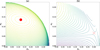 |
Fig. 2 Different topologies on the (e1, e2) plane for different symmetric configurations (a) (θ12, Δϖ12, θ23, Δϖ23) = (0, π, 0, π) and (b) (π, π, 0, 0). The local extrema are (e1, e2, e3) = (0.119,0.1352,0.119) (red solid circle) and (0.300, 0.0662, 0.0671) (red cross), respectively. |
3.2 Topology on eccentricity plane (e1, e2)
Once the semi-major axes a1, a2, and a3 have been determined, the conservation of total angular momentum G restricts the eccentricities e1, e2, and e3 to a two-dimensional plane, and therefore we can consider the topology on a representative eccentricity plane, for example the (e1, e2) plane. An example is illustrated in Fig. 1b. From this plot, a node-like stationary solution located at (e1 e2) = (0.00458, 0.00938) can be found easily. We note that such stationary solutions are just ACRs.
In fact, for different resonant configurations, i.e. different values of (θ12, Δϖ12, θ23, Δϖ23), as well as the total angular momentum G, the Hamiltonian has different structures on the (e1, e2) plane.
For resonant configuration (π, 0, π, π) as shown in Fig. 1, the stationary solution is the local maximum in the (n1/n2, n2/n3) plane, while is the minimum in the (e1, e2) plane, as indicated by colour of the contours. Therefore, the solution is a saddle-like point in the four-dimensional phase space (n1/n2, n2 /n3, e1, e2) and should be considered as unstable.
For resonant configuration (0, π, 0, π), with appropriate eccentricities, the topology on (n1/n2, n2/n3) plane is similar to Fig. 1a, but the topology on (e1, e2) plane, as shown by an example in Fig. 2a, has different features (from Fig. 1b). The stationary solution located at (e1, e2, e3) = (0.119, 0.135, 0.119) now appears as the local maximum and is surrounded by robust energy level curves. The stability of this type ACR will be determined by the topological behaviour on the representative angular plane(s).
Except for the node-like structure on eccentricity plane, we also observe the saddle-like ACR for resonant configuration (π,π, 0,0) as shown in Fig. 2b. It is worth noting that such an ACR appears only for high eccentricities e1 ~ 0.3. Since the saddle-like structure always reveals the orbital instability, these ACRs will not be taken into our consideration.
3.3 Symmetric ACRs
In a symmetric ACR, the critical angle could take either 0 or π. For the 1:2:3 resonant chain, the four critical angles make totally 24 = 16 symmetric configurations. With fixed symmetric resonant angles, period ratios (n1/n2, n2/n3) and the total angular momentum G, we find and locate all the “node-like” (local minimum as in Fig. 1b and local maximum as in Fig. 2a) stationary solution (i.e. ACR) on the eccentricity plane. By varying G, we obtain the symmetric ACR families. The stability of an ACR solution can be determined by analysing the Hamiltonian structure in the two angular planes (θ12, Δϖ12) and (θ23, Δϖ23).
In Fig. 3, on the representative angular planes, we show examples of the Hamiltonian structure for small eccentricity region, where only the symmetric ACRs exist. The saddlelike resonant configuration (θ12, Δϖ12, θ23, Δϖ23) = (π, 0, π, π) marked by the red cross in Fig. 3a is unstable, while the node-like configuration (0, π, 0, π) marked as blue dots is stable.
We calculate the symmetric ACRs for small eccentricity and summarise them in Fig. 4. We note that similar results have been obtained by Antoniadou & Voyatzis (2022) using different methods. For the convenience of comparison, we adopt the same notations of the families and use the following resonant angles:
![Mathematical equation: $\[\left\{\begin{array}{l}\theta_1=2 \lambda_2-\lambda_1-\varpi_1, \\\theta_2=2 \lambda_2-\lambda_1-\varpi_2, \\\theta_3=3 \lambda_3-2 \lambda_2-\varpi_2, \\\theta_4=3 \lambda_3-2 \lambda_2-\varpi_3.\end{array}\right.\]$](/articles/aa/full_html/2024/07/aa49463-24/aa49463-24-eq26.png) (17)
(17)
To distinguish the ACR families belonging to different configurations, we present these symmetric families on the (e1 cos θ1, e2 cos θ2) and (e2 cos θ2, e3 cos θ3) plane. The positive or negative value on the plane indicates that the corresponding resonant angle takes the value of 0 or π.
The ACRs we obtained in Fig. 4 are just the periodic orbits in the rotating frame. Starting from the circular orbit configuration, Antoniadou & Voyatzis (2022) find six symmetric families of periodic orbits, and they denote them by Si, i = 1, ⋯, 6 (“S” for symmetric). We find four of them, namely S2, S3, S5 and S6, of which the critical angles are detailed in Table 1.
As for the two missing families, S1 and S4 in Antoniadou & Voyatzis (2022), their stable segments appear only very shortly when the eccentricities are very small (typically ei ~ 10−6), which makes them less significant since a real planetary system is unlikely to be trapped in such a small-eccentricity configuration and survive for long time span. We failed to detect these two families probably because our semi-analytical Hamiltonian only contains the perturbation up to the first order in the planet-star mass ratio, and the contribution from high-order terms are neglected.
In addition, the symmetric family S5 of configuration (θ12, Δϖ12, θ23, Δϖ23) = (π, 0, π, π) labelled as stable in Antoniadou & Voyatzis (2022) is topologically unstable in our calculation. In fact, the S5 ACR is the local maximum on (n1/n2, n2/n3) plane but local minimum on (e1, e2) plane (e.g. Fig. 1), and such structure holds for the entire family. And we did not find any example that reaches such an orbital configuration in our numerical simulations of the convergent migration (see Sect. 5).
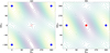 |
Fig. 3 Topology on representative angular planes. The eccentricities of the symmetric ACR are (e1, e2, e3) = (0.00458, 0.00938, 0.00564). (a) Hamiltonian level curves on (θ12, Δϖ12) plane with (θ23, Δϖ23) fixed to (π, π), the saddle-like point at (θ12, Δϖ12) = (π, 0) is marked by a red cross. (b) Topology on (θ23, Δϖ23) plane with (θ12, Δϖ12) fixed to (π, 0). The node-like point at (θ23, Δϖ23) = (π, π) is marked by a red dot. In addition, the stable symmetric configuration (θ12, Δϖ12, θ23, Δϖ23) = (0, π, 0, π) is shown as blue dots. |
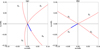 |
Fig. 4 Symmetric ACR families S2, S3, S5, and S6 in the 1:2:3 resonant chain for small-eccentricity configurations on (a) the (e1 cos θ1, e2 cos θ2) plane and (b) the (e2 cos θ2, e3 cos θ3) plane. The stable symmetric ACRs are in blue while the unstable ones in red. The notations of the families are the same as in Antoniadou & Voyatzis (2022), and the resonant angles of different configurations are presented in Table 1. |
3.4 Bifurcation and asymmetric ACRs
As shown in Fig. 4, only the S6 family is stable, and it loses the stability as the eccentricity increases. Along with the increasing eccentricity, the topology around the S6 family varies in a complicated way. An example is illustrated in Fig. 5.
On the (θ12, Δϖ12) plane with fixed (θ23, Δϖ23) = (0, π), the node-like extreme point at (0, π) changes to a saddle-like point while two additional asymmetric ACRs, namely A6 (“A” for asymmetric), arise as the eccentricity increases (Fig. 5a). Meantime, we note that the feature of the node-like structure around (0, π) on the (θ23, Δϖ23) plane with fixed (θ12, Δϖ12) = (0, π) remains the same (Fig. 5b).
The stable asymmetric ACRs are the local extrema of the full phase space (n1/n2, n2/n3, e1, e2, θ12, Δϖ12, θ23, Δϖ23). We adopt the geometrical approach (Michtchenko et al. 2006) to search these asymmetric ACRs in the eight-dimensional space.
All the ACRs are computed under two fixed constants L and G. Since the spacing parameter L only sets the global scale of the system and does not influence the resonant dynamics (except for changing the scales of distance, time, and energy), the evolution of ACRs is in fact parametrised by the constant G, or equivalently, the scaled AMD δ defined as
![Mathematical equation: $\[\delta=\frac{\Gamma_1+\Gamma_2+\Gamma_3}{L}.\]$](/articles/aa/full_html/2024/07/aa49463-24/aa49463-24-eq27.png) (18)
(18)
We summarise in Fig. 6 both the symmetric ACR S6 and the asymmetric ACR A6, in which the evolutions of eccentricities (e1, e2, e3) and resonant angles along these ACR solutions are illustrated.
Along the A6 family, the resonant angles θ12, Δϖ12 between the inner adjacent planets m1, m2 shift significantly from the (unstable) symmetric ACR, while the configuration of the outer planet pair (θ23, Δϖ23) experiences only small variations. Particularly, the angle Δϖ23 remains tightly close to π as δ < 0.01.
Starting from near circular orbits (ei ~ 0), the periodic solution extends to high eccentricity region along the stable branch, blue solid lines first and black dashed lines later in Figs. 6a, b. In a real system, planets in the resonant chain may not revolve exactly along these periodic solutions to high eccentricity, instead, they are expected to be around (but not exactly in) these solutions.
In practice, the numerically averaged Hamiltonian ![Mathematical equation: $\[\bar{\mathcal{H}}\]$](/articles/aa/full_html/2024/07/aa49463-24/aa49463-24-eq28.png) works for arbitrary planetary eccentricities because it does not depend on the literal expansion. Consequently, all the stable ACRs should appear as local extrema in the entire eight-dimensional phase space, and they can be numerically determined by the downhill simplex method under the constraints of fixed L and G. For the 1:2:3 resonant chain, we find more than ten families of stable ACRs at relatively high eccentricity region and they form very complicated structures on the (e1, e2) and (e2, e3) planes. However, further investigations reveal that the topology and the dynamical portraits around these ACR families are similar to each other. Therefore, hereafter we simply focus on the ACR families starting from near circular orbits, namely the S6, A6 family.
works for arbitrary planetary eccentricities because it does not depend on the literal expansion. Consequently, all the stable ACRs should appear as local extrema in the entire eight-dimensional phase space, and they can be numerically determined by the downhill simplex method under the constraints of fixed L and G. For the 1:2:3 resonant chain, we find more than ten families of stable ACRs at relatively high eccentricity region and they form very complicated structures on the (e1, e2) and (e2, e3) planes. However, further investigations reveal that the topology and the dynamical portraits around these ACR families are similar to each other. Therefore, hereafter we simply focus on the ACR families starting from near circular orbits, namely the S6, A6 family.
Critical angles (resonant angles, longitudes of pericentre ϖi, and mean anomalies Mi) of different symmetric resonant configurations.
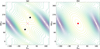 |
Fig. 5 Topology on representative angular planes for symmetric ACR S6 located at (e1e2,e3) = (0.0569, 0.0846, 0.0531). (a) Topology on (θ12, Δϖ12) plane with fixed (θ23, Δϖ23) = (0, π). The saddle-like point at (θ12, Δϖ12) = (0, π) marked by a cross indicates the instability of this solution, while two asymmetric ACRs bifurcated from this unstable symmetric one are indicated by black dots. (b) The topology on (θ23, Δϖ23) plane with (θ12, Δϖ12) fixed to (0, π). The node-like point at (θ23, Δϖ23) = (0, π) is marked by a pink dot. |
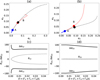 |
Fig. 6 Locations and resonant configurations of the symmetric ACR family (S6) and the asymmetric ACR family (A6). In the upper two panels (a) and (b), the stable symmetric, unstable symmetric, and stable asymmetric ACRs are indicated by blue solid, red solid, and black dashed lines, respectively. Three solid circles on these lines indicate the initial conditions that will be analysed in detail later (see text). The lower two panels (c) and (d) show the evolutions of resonant angles along the asymmetric ACR as the function of δ (scaled AMD, see text). The resonant angles θ12, θ23 and the secular angles Δϖ12, Δϖ23 are labelled by the corresponding lines. |
3.5 Law of structure
As we have shown, for the 1:2:3 resonant chain, the S6−A6 family is the only family that starts from circular orbits and then evolves to highly eccentric configuration. During the evolution from low to high eccentricity along the ACR solution, the mean motion ratios (n1/n2, n2/n3) of the adjacent planet pairs may change. Since these ACR solutions are found by searching for the extrema in the eight-dimensional full space, n1/n2 and n2/n3 are obtained automatically in our calculations. The evolution of these ratios as function of the planets’ eccentricities are summarised in Fig. 7.
As shown in Fig. 7, for the ACR solution, the ratios ni/ni+1 (i = 1, 2) are always above the nominal values (2 and 1.5 in the 1:2:3 resonant chain). Therefore, the planet pairs near the stationary resonant configuration, i.e. in resonance with small oscillations, always have orbital period ratio at one side of the nominal value. The deviation from the nominal value is large for near circular orbits and it decreases for larger eccentricities (thus larger AMD).
The mean motion ratio of the ACR solution depends on planetary masses. Except for the planetary masses as in the Kepler-51 system, we also test two additional systems, in which the planets are 10 and 100 times heavier than the ones in Kepler-51, i.e., keep the mi/mj (i, j = 1, 2, 3) values but set mi/M 10 and 100 times larger than in the Kepler-51 system. Assume they are in the same 1:2:3 resonance chain, we calculate the mean motion ratios, and plot the results in Fig. 7, too. For near circular orbits, the stable ACR solution is symmetric (blue segments in Fig. 7), and from a critical ei it is continued by asymmetric ACR (black segments). Our calculations demonstrate that the critical points for three cases of different total planet masses are the same (e1, e2, e3) = (0.0185, 0.0336, 0.0186), implying the independence of the resonant configuration on the total planetary mass. Indeed, only the mass ratio between adjacent planets influences the resonant configuration (Antoniadou & Voyatzis 2022).
Apparently, for a resonant chain with given mass ratios between planets, the larger the total mass of planets the stronger the short-term perturbations the system would experience. Thus, the resonant chain with higher total planetary mass is more likely to be unstable. The main dynamical mechanism inducing such orbital instability is the 1:1 secondary resonance, which occurs when one of the libration period is almost equal to the period of synodic angle (Pichierri & Morbidelli 2020; Goldberg et al. 2022). This secondary resonance excites the orbital eccentricity and finally destabilises the orbits. In other words, the short term perturbation is too large to be averaged, if the total mass of planets is large enough.
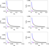 |
Fig. 7 Law of structure for the 1:2:3 resonant chain. The left (right) column of panels show the relation between the mean motion ratio n1/n2 (n2/n3) and the eccentricities (e1, e2, e3 from top to bottom). Blue lines are for the stable symmetric ACR families (S6) while the black lines for the stable asymmetric family (A6). On each panel, the lowest line is for the planets in the Kepler-51 system, while the middle and the top lines are for the cases of 10 and 100 times more massive planets, respectively (see text). The critical points, at which the S6 family becomes unstable and the asymmetric solution appears, are denoted by red crosses. |
4 Dynamics around stable ACRs
For the 1:2:3 resonant chain, the S6−A6 is the only stable family that could evolve from circular orbits to regime of high eccentricity. It is possible that a planetary system may evolve along a “path” guided by the S6−A6 family. In this part, by constructing dynamical maps on the appropriate representative planes, we explore the motion in the vicinity of this evolution path along the S6−A6 ACRs.
4.1 Initial conditions
All the ACR solutions were obtained in the averaged Hamiltonian system, but to construct the dynamical maps we have to use the osculating orbital elements to numerically integrate the orbits. Therefore, we should choose the initial conditions carefully to build a proper association between the averaged system and the real system. Generally, the osculating elements are related to averaged elements by the canonical transformation (see e.g. Ramos et al. 2015; Charalambous et al. 2018, for two-planet and three-planet cases, respectively). But in this paper, we use a simple transformation based on the orbital configuration, particularly the symmetric orbits, as follows.
Typically, the period ratios (n1/n2, n2/n3) of planets inside a resonant chain have only very small oscillation around their nominal value (n1c/n2c, n2c/n3c), otherwise the period commensurability and resonance between planets would break. Therefore, the period ratios, thus the osculating semi-major axes ai, can be fixed at the values of the corresponding stable ACRs āi, that is, ai = āi (i = 1, 2, 3). The same treatment can be applied to eccentricities and resonant angles, ei = ēi (i = 1, 2, 3), ![Mathematical equation: $\[\theta_{i, i+1}=\bar{\theta}_{i, i+1}, \Delta \varpi_{i, i+1}=\overline{\Delta \varpi}_{i, i+1}\]$](/articles/aa/full_html/2024/07/aa49463-24/aa49463-24-eq29.png) (i = 1, 2). In fact, we construct dynamical maps on the (e1, e2) plane with fixed constants L and G defined in Eq. (10). For each point on the (e1, e2) plane, the conversation of L is automatically satified when the semi-major axes a1, a2, a3 were given (in following maps, they were fixed to the values of the exact ACRs), while the eccentricity of the outer planet e3 can be determined through the total angular momentum G. After a1, a2, a3, e1, e2, e3, θ12, Δϖ12, θ23, Δϖ23 have been given as the initial conditions, only one angular variable is left free. We choose the synodic angle Q as the last variable to be determined.
(i = 1, 2). In fact, we construct dynamical maps on the (e1, e2) plane with fixed constants L and G defined in Eq. (10). For each point on the (e1, e2) plane, the conversation of L is automatically satified when the semi-major axes a1, a2, a3 were given (in following maps, they were fixed to the values of the exact ACRs), while the eccentricity of the outer planet e3 can be determined through the total angular momentum G. After a1, a2, a3, e1, e2, e3, θ12, Δϖ12, θ23, Δϖ23 have been given as the initial conditions, only one angular variable is left free. We choose the synodic angle Q as the last variable to be determined.
Let ![Mathematical equation: $\[\left(X_i, Y_i, \dot{X}_i, \dot{Y}_i\right)\]$](/articles/aa/full_html/2024/07/aa49463-24/aa49463-24-eq30.png) be the position and velocity of the i-th body mi in the rotational frame. An orbit starting from the GX axis at time t0 = 0 and satisfying Xi(t0) ≠ 0,
be the position and velocity of the i-th body mi in the rotational frame. An orbit starting from the GX axis at time t0 = 0 and satisfying Xi(t0) ≠ 0, ![Mathematical equation: $\[\dot{X}_i\left(t_0\right)\]$](/articles/aa/full_html/2024/07/aa49463-24/aa49463-24-eq31.png) = 0, Yi(t0) = 0,
= 0, Yi(t0) = 0, ![Mathematical equation: $\[\dot{Y}_i\left(t_0\right)\]$](/articles/aa/full_html/2024/07/aa49463-24/aa49463-24-eq32.png) ≠ 0 (i = 1, 2, 3) is symmetric with respect to the GX axis, because the symmetric condition Eq. (6) is apparently fulfilled. The algebraic manipulation reveals that the symmetry in the rotational frame leads to
≠ 0 (i = 1, 2, 3) is symmetric with respect to the GX axis, because the symmetric condition Eq. (6) is apparently fulfilled. The algebraic manipulation reveals that the symmetry in the rotational frame leads to
![Mathematical equation: $\[\begin{aligned}& \left|\boldsymbol{r}_i(t)-\boldsymbol{r}_j(t)\right|=\left|\boldsymbol{r}_i(-t)-\boldsymbol{r}_j(-t)\right|, \\& \boldsymbol{p}_i(-t) \cdot \boldsymbol{p}_j(-t)=\boldsymbol{p}_i(t) \cdot \boldsymbol{p}_j(t).\end{aligned}\]$](/articles/aa/full_html/2024/07/aa49463-24/aa49463-24-eq33.png) (19)
(19)
Thus, the Hamiltonian ![Mathematical equation: $\[\mathcal{H}\]$](/articles/aa/full_html/2024/07/aa49463-24/aa49463-24-eq34.png) should follow the same symmetry
should follow the same symmetry ![Mathematical equation: $\[\mathcal{H}\]$](/articles/aa/full_html/2024/07/aa49463-24/aa49463-24-eq35.png) (−t) =
(−t) = ![Mathematical equation: $\[\mathcal{H}\]$](/articles/aa/full_html/2024/07/aa49463-24/aa49463-24-eq36.png) (t). Since
(t). Since ![Mathematical equation: $\[\mathcal{H}\]$](/articles/aa/full_html/2024/07/aa49463-24/aa49463-24-eq37.png) depends explicitly on rather Q than t, while Q is a linear function of t, up to the 1st order of the planet-star mass ratio (m1 + m2 + m3)/M, we have
depends explicitly on rather Q than t, while Q is a linear function of t, up to the 1st order of the planet-star mass ratio (m1 + m2 + m3)/M, we have ![Mathematical equation: $\[\mathcal{H}\]$](/articles/aa/full_html/2024/07/aa49463-24/aa49463-24-eq38.png) (−Q) =
(−Q) = ![Mathematical equation: $\[\mathcal{H}\]$](/articles/aa/full_html/2024/07/aa49463-24/aa49463-24-eq39.png) (Q). Therefore, the Hamiltonian must be symmetric with respect to Q0 = Q(t = 0) and
(Q). Therefore, the Hamiltonian must be symmetric with respect to Q0 = Q(t = 0) and ![Mathematical equation: $\[\mathcal{H}\]$](/articles/aa/full_html/2024/07/aa49463-24/aa49463-24-eq40.png) (Q0) must be an extremum. To determine the proper osculating orbital elements, we need to find the appropriate Q, and now it is equivalent to find the Q at which
(Q0) must be an extremum. To determine the proper osculating orbital elements, we need to find the appropriate Q, and now it is equivalent to find the Q at which ![Mathematical equation: $\[\mathcal{H}\]$](/articles/aa/full_html/2024/07/aa49463-24/aa49463-24-eq41.png) (Q) reaches the extrema.
(Q) reaches the extrema.
We plot in Fig. 8 the variation of the Hamiltonian with respect to the synodic angle Q for both symmetric and asymmetric resonant configurations. It is clear that the Hamiltonian is symmetric with respect to the red vertical line in Fig. 8a, which corresponds to the global minimum. The above calculations can be applied to all the symmetric ACRs, and all the angles (ϖi, Mi) (i = 1, 2, 3) at the symmetric solutions have been summarised in Table 1.
For asymmetric configurations, as shown in Fig. 8b, the symmetry condition cannot be fulfilled. The Q value, at which the Hamiltonian attains the minimum, is calculated and adopted as the initial configuration.
 |
Fig. 8 Variation of the Hamiltonian in two synodic periods |
![Mathematical equation: $\[2 Q_{12}^T=12 \pi\]$](/articles/aa/full_html/2024/07/aa49463-24/aa49463-24-eq42.png)
4.2 Max (Δ e) indicator and χ2 criterion
For each point on the (e1, e2) plane, we numerically integrate the equations of motion up to 105 yr from the corresponding initial conditions (osculating elements). We note that the “year” here is defined as the orbital period of the middle planet m2. During the integration, we keep tracking the maximal and minimal values attained by the planetary eccentricities and adopt the variation range (Δe1, Δe2, Δe3) as the indicator to characterise the orbital stability. As mentioned in Ramos et al. (2015), although the Δe is not a rigorous measure of chaos of the motion, it’s a useful tool for the estimation of both the possible fixed points and the dynamical separatrix of the resonant region. In practise, we may consider the orbits with small Δe as “stable” and the ones with large Δe as “chaotic” (close to the dynamical separatrix).
In a two-body MMR, after the numerical averaging over the synodic angle Q, the system is reduced to a Hamiltonian of only 2 DoF. The existence of the resonant invariant torus, or dynamical separatrix (Alves et al. 2016), forbids the transition between the resonant and the non-resonant region. Inside the resonant zone, the resonant angles librate around the ACR solutions, while they circulate outside the resonant region. Thus, different types of motion can be easily distinguished from each other. Unfortunately, in the three-planet resonant system, the resonant angles behave in a much more complicated way. Due to the perturbation from the third planet, a two-body resonant angle may librate irregularly with a large amplitude and appear like in a complex of both libration and circulation. As a result, it’s difficult to determine accurately whether the system is in a resonance (or dominated by the resonance). Following the idea by Gallardo (2014), another indicator, χ2 of the resonant angles, is used in this paper.
The indicator χ2 is defined to characterise different effects of the resonance in a three-planet system: deep in resonance (resonant angles librating), at the boundary of resonance (resonant angles circulating or librating with large amplitudes), and outside resonance.
The basic idea is to analyse the resonant angle over a period of time T*. The statistical difference χ2 between the distributions of a resonant angle and a uniform distribution in [−π, π] is adopted as an indicator to determine whether the system is in a resonance: the larger the χ2, the more likely the resonance angle is in libration, and vice versa.
The semi-quantitative criterion will be given through a standard pendulum model with Hamiltonian:
![Mathematical equation: $\[\mathcal{H}_{\text {pend }}=\frac{p_{\varphi}^2}{2}-\cos \varphi.\]$](/articles/aa/full_html/2024/07/aa49463-24/aa49463-24-eq43.png) (20)
(20)
From each point of a 100 × 100 grid on the phase space [pφ, φ] ∈ [−4, 4] × [−π, π], we integrate the corresponding Hamiltonian equations and output N = 213 = 8192 points ![Mathematical equation: $\[\left\{\varphi_i\right\}_{i=1}^{N=8192}\]$](/articles/aa/full_html/2024/07/aa49463-24/aa49463-24-eq44.png) evenly in a time step Δt = 5. The interval [−π, π] is divided into 180 equal bins, and the χ2 of such an orbit is computed as
evenly in a time step Δt = 5. The interval [−π, π] is divided into 180 equal bins, and the χ2 of such an orbit is computed as
![Mathematical equation: $\[\chi^2=\sum_{k=1}^{180} \frac{\left(O_k-E_k\right)^2}{E_k},\]$](/articles/aa/full_html/2024/07/aa49463-24/aa49463-24-eq45.png) (21)
(21)
where Ok is the number of φi observed in the k-th bin, and Ek is the expected number in the same bin if the 8192 values are in a uniform distribution. We show in Fig. 9 the phase space of the standard pendulum and the χ2 map.
Apparently, all the points located inside the libration region in Fig. 9 have χ2 > 1 (log χ2 > 0), while those points with χ2 < 0.1 are surely in the circulation region. For initial conditions in the close vicinity of the separatrix, their orbital periods are so long that the total integration time could not cover several times of their periods and therefore, some orbits in the circulation region might be misunderstood as “libration”. Empirically, the resonant behaviours can be estimated by the value of χ2:
χ2 > 1, the resonant angle is in libration and the system is deeply inside the resonance;
χ2 < 0.1, the resonant angle is in circulation and the system is outside the resonance;
0.1 < χ2 < 1, the system is affected by the resonance, but the resonant angles may experience both the libration and circulation in a long time span. We classify this behaviour as the motion near the separatrix.
For the MMR between planets mi, mj, the resonance is characterised by the libration of at least one of the resonant angles
![Mathematical equation: $\[\theta_{i j}^l=k_{j i} \lambda_j-k_{i j} \lambda_i-l \varpi_i-\left(q_{i j}-l\right) \varpi_j, \quad l=0,1, \cdots, q_{i j},\]$](/articles/aa/full_html/2024/07/aa49463-24/aa49463-24-eq46.png) (22)
(22)
where qij = |kij − kji| is the order of the resonance, and the librating angle is referred as the true resonant angle (Alves et al. 2016). Therefore, the criterion χ2 of an MMR is defined as the largest χ2 value of all resonant angles, and we may adopt the same empirical criterion obtained in the pendulum model.
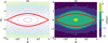 |
Fig. 9 χ2 map for the standard pendulum model, (a) Phase structure (energy level) on (φ, pφ) plane. The broad red curve marks the separatrix between the libration and circulation region, (b) χ2 value in logarithm indicated by colour. |
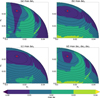 |
Fig. 10 Topology (contour line) and dynamical map (colour map) on the (e1, e2) plane for Case A, with constants L and G determined by the initial condition on the stable ACR solution (e1, e2, e3, θ12, Δϖ12, θ23, Δϖ23) = (0.0124, 0.0237, 0.0128, 0, π, 0, π), which is indicated by a red dot on all maps. The eccentricity variations Δei are used as the stability indicator as labelled in each panel. |
4.3 Motion around symmetric ACRs at low eccentricity
Along the S6−S6 family, the symmetric ACR solution is stable at low eccentricity (Fig. 6). Arbitrarily, we select on the ACR one initial condition (e1 e2, e3) = (0.0124, 0.0237, 0.0129), which is labelled by ‘A’ in Fig. 6. The resonant angles of this solution are (θ12, Δϖ12, θ23, Δϖ23) = (0, π, 0, π), and the period ratios are set as the nominal values in the 1:2:3 resonant chain. Keeping the constant L and G calculated from the above ai, ei(i = 1, 2, 3), we generate a set of initial conditions both for the averaged Hamiltonian system and for the corresponding osculating system. We denote the case with these initial conditions by “Case A”, and investigate the motion.
We present in Fig. 10 on the (e1, e2) plane both the topologies (contour curves) of the corresponding averaged Hamiltonian and the dynamical maps (coloured map) obtained from numerical integration of the osculating orbital elements. The ACR solution appears as the local maximum and is surrounded by ellipse-like energy curves, implying its stability. The maximum of the eccentricity variation Δei is adopted as the indicator of stability as labelled on each panel in Fig. 10. And particularly, the maximum of (Δei, Δe2, Δe3) is used in the last panel.
As clearly shown in Fig. 10, all the four maps reveal that the motion is very stable around the ACR with very small eccentricity variations. Further analyses show that these stable orbits are characterised by the libration around the stable ACR, performing the so called quasi-periodic motion. As a matter of fact, such a regular region can occupy a large area on the (e1, e2) plane.
Away from the stable ACR, the dynamical maps of different indicators may show different patterns. The region of small Δe1 and Δe2 extends roughly along either the e1 (horizontally) or the e2 direction (vertically). At about (e1, e2) = (0.025, 0.02) in Fig. 10a, the planet m1 would suffer relatively large eccentricity excitation (Δe1 > 0.02) and the corresponding orbit is much less regular. In addition, starting from about (e1, e2) = (0.032, 0.006) we also notice a very narrow strip with relative large value of Δe1.
The dynamical features in Figs. 10b,c for Δe2 and Δe3 are similar. At the bottom of the (e1, e2) plane, Δe2 attains its maximum value (~0.04), implying (relatively) the least stability of motion there. And in all three panels a, b and c, deviated from the ACR, regular region can also be found at the right corner of (e1, e2) plane, where motions are distinct from the quasi-libration around the ACR.
Finally, we find that all these dynamical features can be revealed by the maximum of the three eccentricity variations, i.e. max(Δe)= max(Δe1, Δe2, Δe3), as shown in Fig. 10d. Particularly, we see in Fig. 10d that the most stable motions occur in three regions, around the ACR, around (e1, e2) = (0.032, 0.017), and around (0.04, 0.01), respectively. Below in this paper, we adopt max(Δe) as the stability indicator and construct the dynamical maps.
The χ2 maps might provide more details on the resonant dynamics. In Fig. 11, we depict the χ2 maps for all the MMRs inside the 1:2:3 resonant chain. For all MMRs, the closer to the stable ACR, the larger the χ2, implying that in the close vicinity of the stable ACR solution, all the resonant angles are librating, as well as the three-body Laplace resonant angle. The regular motion, characterised by the quasi-periodic libration around the ACR, is common around the ACR solution.
The χ2 maps in Fig. 11 reveal that, as e1 increases (while e2 remains the value of ACR), the 2:3 two-body resonance (MMR23) in the outer planet pair persists and seems to play an essential role to the resonant stability, while other resonances in the resonant chain are weaken or even destroyed. The region with small Δe2 in Fig. 10b coincides with the region of χ2 > 1 in Fig. 11b. When e2 deviates from the ACR value (with e1 almost being frozen), the inner planet pair’s 1:2 resonance (MMR 12), the 1:3 resonance (MMR 13) between m1 and m3, and the three-planet Laplace resonance, persist in a range of e2, as shown by the vertical strip-like structures of large χ2 in Figs. 11a, c, d. Therefore, away from the ACR solution along the direction of e1, although the MMR23 is stable, the strength of MMR12, MMR13, and Laplace resonance becomes weaker, implying that the corresponding resonant angles may librate with large amplitudes and eventually the Laplace angle φ0 will be in circulation.
A nearly vertical narrow strip of small χ2 that divides the stable region into two parts, namely Region 1 and Region 2, can be seen in Figs. 11a, c, the separatrix-like structure corresponds to the broad region with large Δe1 on the dynamical map (Fig. 10a). We check carefully the motion in these two regions and find that the orbits in Region 1 are librating around the stable ACR (Fig. 12), while in Region 2, although all the two-body MMRs (i.e. MMR 12, MMR23, and MMR 13) occur, the Laplace angle φ0 circulates (Fig. 13), as indicated by the small χ2 value in the area of Region 2 in Fig. 11d.
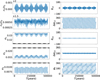
A typical example of orbits in Region 1 is displayed in Fig. 12. The mean motion ratios n1/n2, n2/n3 librate with very small amplitudes around the nominal values (2 and 1.5), implying that the semi-major axes are almost constants. The eccentricities e1, e2, e3 oscillate around the periodic solution (symmetric ACR, indicated by horizontal lines in the corresponding panels). And the tiny libration of critical resonant angles (including the Laplace angle) around 0° or 180° reveals that the motion is deeply in the resonant chain, even we know that the initial condition is not exactly on the ACR solution.
But for orbits in Region 2, as shown in Fig. 13, the resonant angles of MMR12 and MMR23, i.e. θ12 and θ23, librate around 0° with very small amplitude, as well as the apsidal difference Δϖ23 librates around 180°. As a result, the resonant angle of MMR13, ![Mathematical equation: $\[\theta_{13}^1=\theta_{12}+\theta_{23}+\Delta \varpi_{23}=3 \lambda_3-\lambda_1-\varpi_1-\varpi_3\]$](/articles/aa/full_html/2024/07/aa49463-24/aa49463-24-eq47.png) (see Eq. (22) for the definition) librates and the system is surely in the MMR between the non-consecutive planets m1 and m3. However, due to the circulation of Δϖ12, the Laplace angle φ0 = θ12 − θ23 − Δϖ12 eventually circulates, indicating that the system is not in the three-body MMR. The eccentricities of the stable ACR solution are also plotted in Fig. 13, in which it can be seen that all e1, e2 and e3 are far away from these ACR values. This implies that the typical orbit in Region 2 is no longer librating around the stable ACR. The motion in Region 2 in fact follows a new stable mode in the resonant chain, in which the dynamics is actually dominated by the individual two-body MMRs. Since in such a configuration each pair of planets is in the corresponding two-body MMR but the three-planet Laplace resonance does not happen, we refer to this type of configuration as “joint two-body resonance”.
(see Eq. (22) for the definition) librates and the system is surely in the MMR between the non-consecutive planets m1 and m3. However, due to the circulation of Δϖ12, the Laplace angle φ0 = θ12 − θ23 − Δϖ12 eventually circulates, indicating that the system is not in the three-body MMR. The eccentricities of the stable ACR solution are also plotted in Fig. 13, in which it can be seen that all e1, e2 and e3 are far away from these ACR values. This implies that the typical orbit in Region 2 is no longer librating around the stable ACR. The motion in Region 2 in fact follows a new stable mode in the resonant chain, in which the dynamics is actually dominated by the individual two-body MMRs. Since in such a configuration each pair of planets is in the corresponding two-body MMR but the three-planet Laplace resonance does not happen, we refer to this type of configuration as “joint two-body resonance”.
It is worth noting that a separatrix-like structure indicated by the red arrow in Fig. 11a further splits Region 2 into two subregions. But the orbits from both sides of this structure are very similar to each other, characterised by libration of θ12, θ23, θ113 and circulation of φ0. The only difference between orbits from two sides is the oscillation centres of eccentricities, (e1, e2, e3) ≈ (0.032, 0.017, 0.009) for the left side (as the one shown in Fig. 13) and (e1 e2, e3) ≈ (0.040, 0.012, 0.007) for the right side. Most probably, such a fine structure in Region 2 is attributed to the nonlinear terms in the perturbation (Rath et al. 2022). We also note that the corresponding structure can also be found in the map of maximum of eccentricity variation (Fig. 10).
Finally, at the bottom of the dynamical map (Fig. 10 at e2 ~ 0), we observe a thin region with a large eccentricity variation. The eccentricities (e2, e3) in this thin region are excited mainly because the outer two-body MMR (MMR23) is close to its boundary, as indicated by the small χ2 value in the bottom area in Fig. 11b.
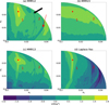 |
Fig. 11 Resonant structure indicated by χ2 on the (e1, e2) plane for Case A. Four panels are for the two-body MMRs between (a) m1 and m2, (b) m2 and m3, (c) m1 and m3, and (d) the three-planet Laplace resonance with resonant angle φ0. The large value of χ2 (light colour) indicates that the resonant angle is in libration, while the small χ2 (dark tones) indicates circulation. The narrow strip-like structure indicated by a black arrow in (a) divides the map into two parts, namely Region 1 and Region 2. Moreover, another narrow strip (indicated by the red arrow) can be seen in Region 2. |
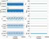 |
Fig. 12 Typical behaviour of the orbits in Region 1 (Fig. 11a). The temporal variations of n1/n2, n2/n3, e1, e2, e3 are in left panels, while right panels are for resonant angles θ12, Δϖ12, θ23, Δϖ23, φ0. The orbits are librating quasi-periodically around the stable symmetric ACR solution S6. The eccentricities of S6 are indicated by horizontal dashed lines. |
4.4 Motion around asymmetric ACRs at moderate eccentricity
The symmetric ACR solution loses its stability at a specific point, and it bifurcates into two asymmetric ACR solutions. We select again arbitrarily an initial condition from the asymmetric ACR branch, and perform the similar calculations as for the symmetric case. The eccentricities at this initial point, indicated by the black solid circle labelled “B” in Fig. 6, are (e1, e2, e3) = (0.0602, 0.0903, 0.0440). We call this case “Case B”.
The resonant angles at this initial point of asymmetric ACR are (θ12, Δϖ12, θ23, Δϖ23) = (26.7°,−119.5°, 1.16°, 179.5°). From these initial values, we obtain the corresponding constants L and G. For comparison we also calculate the unstable symmetric ACR solution with the same L and G, of which the eccentricities and resonant angles are (0.0569, 0.0846, 0.0531, 0, 180°, 0, 180°), i.e. the red solid circle in Fig. 6. Then, for both of these two initial conditions, we calculate the topology and dynamical maps, and present them in Fig. 14. In this figure, the max(Δe) is chosen as the stability indicator.
Comparing the two panels in Fig. 14, we find that the topology of the unstable symmetric ACR is similar to the one of the stable asymmetric ACR, but their dynamical maps show different patterns. The non-zero values of max(Δe) ~ 0.04 at the close proximity of the unstable symmetric ACR in Fig. 14a implies the orbits there deviate from the unstable stationary solution in the evolution. On the contrary, the stable asymmetric ACR in Fig. 14b is surrounded by regular orbits as indicated by the max(Δe) ~ 0.
A closer look at the orbits around the unstable symmetric ACR reveals that they are still in resonance, librating around both the asymmetric ACRs and the symmetric ACR with large amplitude, in a way similar to the horseshoe orbit around the Lagrange points L4 − L3 − L5 in the circular restricted three-body problem (see e.g. Murray & Dermott 2000). One typical orbit in that region is shown in Fig. 15. Although it behaves chaotically due to the instability of symmetric ACR, the libration of the resonant angles indicate that the motion is still inside the resonant chain after the end of the numerical integration. Such horseshoe-like orbits can surely survive in the resonant chain in the long term.
On the other hand, the orbits near the stable asymmetric ACR solution are in a regular area (Fig. 14b), and they are protected by the resonant chain. We present in Fig. 16 the χ2 map on the representative plane where all the initial resonant angles are fixed as the ones of the asymmetric ACR solution. As can be seen in Fig. 16, the close proximity around the stable ACR is deeply involved in the MMRs, as indicated by the large χ2 value (yellow colour). Consistent with the dynamical map in Fig. 14b, such regular region occupies large phase space, with the eccentricities e1, e2 extending to e1 → 0.1, e2 → 0.1. For orbits inside the yellow region (χ2 > 10) in Fig. 16, the libration amplitudes of resonant angles θ12, θ23 are smaller than 10°. As a consequence, some three-body resonant angles Ψ[M,N] = Mθ12 + Nθ23 librate. We note that the libration of Ψ in this case does not indicate a “real” three-planet resonance but is the necessary consequence of the libration of two-body resonance angles.
Similar to the resonant structure near the stable symmetric ACR (Fig. 11), the librating region of MMR23 extends in the e1 (but not e2) direction while the one of MMR12 extends along the e2 direction. The MMR between planets m1, m13 (MMR13) and the Laplace resonance appear as the intersection of MMR12 and MMR23. With increasing displacement from the ACR, we notice a broad stripe with small χ2 in Fig. 16a that divides the libration zone into two parts, namely Region 1 and Region 2 again. This type of “chaotic border” is similar to the one in Fig. 11a for Case A. And it has apparent correspondence in the dynamical map in Fig. 14b for Case B.
Judging from the χ2 value, the orbits in Region 1 are involved in all three two-body MMRs and the three-body Laplace resonance. The motion is nearly the same as the one in Case A shown in Fig. 12, only except that the resonance centre is at the asymmetric values. Close to the ACR solution, the motion is regular, and departing away from the ACR the irregularity increases, as shown by the max(Δe) value in Fig. 14b. However, in Region 2, which is far away from the ACR solution, the small max(Δe) value indicates that the motion is regular, although the χ2 value implies that some resonances have broken. To show the orbital behaviour in Region 2, we illustrate a typical example in Fig. 17.
As shown in Fig. 17, the period ratios n1/n2, n2/n3 still stay close to the nominal values (2,1.5). The eccentricities oscillate regularly around the centre ![Mathematical equation: $\[\left(e_1^*, e_2^*, e_3^*\right)=(0.19,0.072,0.035)\]$](/articles/aa/full_html/2024/07/aa49463-24/aa49463-24-eq48.png) that is quite far away from the ACR solution. Instead of librating around the ACRs (the unstable symmetric one and the two stable asymmetric ones), the resonant angles behave in a similar way as the ones in Case A illustrated in Fig. 13, that is, all the two-body MMRs occur (at least one of the corresponding resonant angles librates) while the three-body Laplace resonance does not (φ0 circulates). Therefore, the “joint two-body resonance” happens in this region of (relatively) high eccentricity.
that is quite far away from the ACR solution. Instead of librating around the ACRs (the unstable symmetric one and the two stable asymmetric ones), the resonant angles behave in a similar way as the ones in Case A illustrated in Fig. 13, that is, all the two-body MMRs occur (at least one of the corresponding resonant angles librates) while the three-body Laplace resonance does not (φ0 circulates). Therefore, the “joint two-body resonance” happens in this region of (relatively) high eccentricity.
The orbits of “joint two-body resonance” found in both Cases A and B (Figs. 13 and 17) reveal that this configuration can occur in a wide range of initial conditions. We note that this type of mode of stable “joint two-body resonance” is missed in our averaged model, i.e. the motion is not the resonant periodic orbits, but it is a common outcome from planetary migration and tidal dissipation, as shown in Morrison et al. (2020).
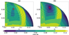 |
Fig. 14 Same as Fig. 10 but for Case B. The constants L and G are determined by the initial condition on the stable asymmetric ACR solution (black solid circle in Fig. 6). (a) Around the unstable symmetric ACR solution with the same L, G. The corresponding eccentricities e1, e2, e3 are 0.0569, 0.0846, 0.0531 (red solid circle in Fig. 6). (b) Around the stable asymmetric ACR solution. The colour in both panels indicates the value of max(Δe). |
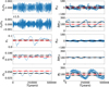 |
Fig. 15 Horseshoe-like orbit near the unstable symmetric ACR. The unstable symmetric ACR and the stable asymmetric ACRs are indicated by the red and black horizontal lines, respectively. |
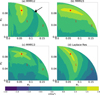 |
Fig. 16 Same as Fig. 11 but for Case B. The map is divided into two parts (Region 1 and Region 2) by a stripe-like structure of relatively smaller χ2 value, as indicated by the arrow in panel a. |
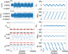 |
Fig. 17 Same as Fig. 13 but the initial conditions are from the high eccentricity region of Fig. 14 (see text). |
4.5 Stable motion inside the 1:2:3 resonant chain
Basically, in the close neighbourhood of the ACR solutions as we have investigated in this paper, two types of stable motion of the 1:2:3 resonant chain can be found. One is the stable ACR (resonant periodic orbits) and the associated quasi-periodic motion, where all the resonant angles, including the two-body MMRs and the Laplace resonance angle, are librating (χ2 > 1). The other one is the “joint two-body MMR”, where θ12, θ23 and ![Mathematical equation: $\[\theta_{13}^1\]$](/articles/aa/full_html/2024/07/aa49463-24/aa49463-24-eq49.png) are librating while the Laplace angle φ0 circulates. Judging from the dynamical maps and our long-term numerical simulations, the difference in stability between these two types of motion is negligible. Therefore, in the close vicinity of the nominal resonance, we might conclude that the individual two-body MMRs dominate the stability of the 1:2:3 resonant chain, while the libration of the three-body Laplace angle is not a necessary condition of the resonant chain but a necessary outcome of the two-body resonant angles’ librating.
are librating while the Laplace angle φ0 circulates. Judging from the dynamical maps and our long-term numerical simulations, the difference in stability between these two types of motion is negligible. Therefore, in the close vicinity of the nominal resonance, we might conclude that the individual two-body MMRs dominate the stability of the 1:2:3 resonant chain, while the libration of the three-body Laplace angle is not a necessary condition of the resonant chain but a necessary outcome of the two-body resonant angles’ librating.
This feature can be explained through the Hamiltonian model. The perturbed part ![Mathematical equation: $\[\mathcal{H}\]$](/articles/aa/full_html/2024/07/aa49463-24/aa49463-24-eq50.png) 1 of Hamiltonian in Eq. (7) only contains the interactions between each two planets. After the numerical averaging process (eliminating all the non-resonant term), up to the 1st order in planet-star mass ratio, the final averaged Hamiltonian
1 of Hamiltonian in Eq. (7) only contains the interactions between each two planets. After the numerical averaging process (eliminating all the non-resonant term), up to the 1st order in planet-star mass ratio, the final averaged Hamiltonian ![Mathematical equation: $\[\bar{\mathcal{H}}\]$](/articles/aa/full_html/2024/07/aa49463-24/aa49463-24-eq51.png) in Eq. (13) only contains the terms induced by the two-body MMRs but not the three-body resonance. Consequently, for a planetary system close to a resonant chain, the dynamics is mainly dominated by the two-body MMRs.
in Eq. (13) only contains the terms induced by the two-body MMRs but not the three-body resonance. Consequently, for a planetary system close to a resonant chain, the dynamics is mainly dominated by the two-body MMRs.
Therefore, if we can verify that a planetary system locates inside all the two-body MMRs (at least one critical resonant angle librates for each MMR), no matter how the Laplace angle φ0 behaves, we will know for sure that the resonant chain is formed. In the practice of dynamical studies, the χ2 indicator can distinguish libration from circulation and thus provide the priori estimation of the stability in short-time numerical integration (only up to tens of resonant periods, empirically 104−105 synodic periods), which is in fact easy to perform.
In addition, the three-body Laplace resonant angle φ0 can be easily detected in transit data. Once the orbital periods and semi-major axes of the planets are determined, the behaviour of φ0 is often adopted as an indicator to probe whether the planetary system is involved in a resonant chain (e.g. Jontof-Hutter et al. 2016). According to our analyses of the 1:2:3 resonant chain, the libration of the three-body resonant angle can almost ensure that the system is librating around a certain ACR. In this case, the dynamics and the possible behaviours of the orbital elements can be explained and predicted by studying the Hamiltonian topology and the dynamical maps on appropriate representative planes.
If a system is not in the close vicinity of the nominal resonances, i.e. if the offset from the exact period commensurability is considerable, the pure three-body MMRs (with absence of any two-body MMR) may play its role. Recently, Rath et al. (2022) propose an analytical model (perturbed pendulum) of the chaotic dynamics near the resonant chain, and they demonstrate that the pure three-body resonances should appear as the secondary resonance with the critical angle defined as Ψ[M,N] = Mϕ + Nψ, where ϕ and ψ are the critical angles of individual two-body MMRs:
![Mathematical equation: $\[\phi=k_{21} \lambda_2-k_{12} \lambda_1, \quad \psi=k_{23} \lambda_2-k_{32} \lambda_3.\]$](/articles/aa/full_html/2024/07/aa49463-24/aa49463-24-eq52.png) (23)
(23)
It is important to note that the ϖ terms have been neglected. Obviously, the [M,N]=[1,1] type is the largest secondary resonance (for the example of the 1st order three-body resonance, see Cerioni & Beaugé 2023). For the 1:2:3 resonant chain, it’s just the Laplace resonance φ0 = λ1 − 4λ2 + 3λ3. Specifically for the 1:2:3 resonant chain, Antoniadou & Voyatzis (2022) find the stable region associated with this zeroth-order three-body resonance. However, we did not detect these configuration, perhaps because our initial condition are always chosen at exact nominal resonance. More efforts are needed to investigate how the pure three-body resonance affects the resonant configuration and the long term stability.
5 Resonant configuration via convergent migration
So far, we have shown both by the Hamiltonian method and by numerical simulations what the orbital configurations might be in a planetary resonant chain. Generally, an MMR between two planets can be easily attained via planetary convergent migration, which can also lead multiple planets to form a resonant chain and then to achieve an orbital configuration of high eccentricity (see e.g. Voyatzis 2016). In this section, we study whether the orbital configurations we have analysed above can be attained through convergent migration of planets.
Due to the interaction between the planet and the circumstellar disk (gaseous disk or planetesimal disk), the migration of planet is quite common. For simplicity, in this paper the migration is simulated by adding an artificial dissipative force on the planet. Specifically, the torque acting on the i-th planet is assumed as (see e.g. Delisle et al. 2015):
![Mathematical equation: $\[\ddot{\boldsymbol{r}}_i=-\left[\frac{\boldsymbol{v}_i}{2 \tau_{a, i}}+\frac{2\left(\boldsymbol{v}_i \cdot \boldsymbol{r}_i\right) \boldsymbol{r}_i}{r_i^2 \tau_{e, i}}\right],\]$](/articles/aa/full_html/2024/07/aa49463-24/aa49463-24-eq53.png) (24)
(24)
where ri, υi are the position and velocity vector, and τa,i,τe,i are timescales of orbital migration and eccentricity damping, for the ith planet. Up to the first order in eccentricity, the effects of the dissipative force on the planetary semi-major axis and eccentricity read:
![Mathematical equation: $\[a_i(t)=a_i(t=0) \exp \left(-\frac{t}{\tau_{a, i}}\right), e_i(t)=e_i(t=0) \exp \left(-\frac{t}{\tau_{e, i}}\right).\]$](/articles/aa/full_html/2024/07/aa49463-24/aa49463-24-eq54.png) (25)
(25)
Constant timescales were adopted in our simulations, and in order to fulfil the global convergent condition (e.g. Beaugé & Cerioni 2022; Wong & Lee 2024), different migration parameters will be chosen for different resonant chains.
5.1 1:2:3 resonant chain
To reach the 1:2:3 resonant chain, following Beaugé & Cerioni (2022), we assumed that all three planets migrated inwards and the migration timescales τa,i were set to be 0.5, 0.2, 0.1 Gyr for planets m1, m2 and m3. The eccentricity damping timescales τe,i were set in such a way that for each planet κ = τa,i/τe,i = 50. As we did for the dynamical maps, the initial semi-major axis of m2 is set to be a2 = 1 AU. All planets start from coplanar and circular orbits and the initial period ratios T2/T1 and T3/T2 are set in a 15 × 15 grid in the ranges of [2.01, 2.02] and [1.51, 1.53]. The initial angles ϖi, λi were all set to be 0°. This choice corresponds to a collinear configuration, in which the mutual distances between planets are minimum. All the orbits starting from the 225 initial conditions were then integrated for a total time span of T = 107 yr.
During the numerical integrations, we keep tracking the behaviour of the resonant offset Δij = ni/nj − kj/ki between the adjacent planets. Once all the resonant offsets are smaller than a given level ![Mathematical equation: $\[\Delta_{i j}^c\]$](/articles/aa/full_html/2024/07/aa49463-24/aa49463-24-eq55.png) , we then monitor the behaviour of resonant angles by checking their χ2 and classify the motion. It should be noted that the critical
, we then monitor the behaviour of resonant angles by checking their χ2 and classify the motion. It should be noted that the critical ![Mathematical equation: $\[\Delta_{i j}^c\]$](/articles/aa/full_html/2024/07/aa49463-24/aa49463-24-eq56.png) can be chosen empirically, and after some tests, we set
can be chosen empirically, and after some tests, we set ![Mathematical equation: $\[\Delta_{i j}^c\]$](/articles/aa/full_html/2024/07/aa49463-24/aa49463-24-eq57.png) = 20 × (m1 + m2 + m3)/M × kj/ki.
= 20 × (m1 + m2 + m3)/M × kj/ki.
For the 1:2:3 resonant chain, we found that only two types of resonant configuration are achievable in our numerical simulations. The first one is that the planetary system attains the resonant chain and eventually librates around the stable ACR solutions (S6, A6). One such example is shown in Fig. 18. As the planets migrate, both period ratios n1/n2 and n2/n3 decrease, while the eccentricities remain close to zero. After the system reaches the 1:2:3 resonant chain at t ≈ 106 yr, the period ratios are subsequently locked into the resonance and the eccentricities are excited from then on. Meanwhile, all the angles begin to librate around the values of the symmetric ACR, (θ12, Δϖ12, θ23, Δϖ23) = (0, π, 0, π), i.e. the S6 family. Once the bifurcation point is reached at t ≈ 2.4 × 10⁶ yr, the system follows the asymmetric family A6 and finally librates around the asymmetric ACR at about ![Mathematical equation: $\[\left(e_1^*, e_2^*, e_3^*, \theta_{12}^*, \Delta \varpi_{12}^*, \theta_{23}^*, \Delta \varpi_{23}^*)\right.\]$](/articles/aa/full_html/2024/07/aa49463-24/aa49463-24-eq58.png) = (0.0371, 0.0623, 0.0345, 24.6°, −133.5°, 0.5°, 178.9°).
= (0.0371, 0.0623, 0.0345, 24.6°, −133.5°, 0.5°, 178.9°).
The second one is the “joint two-body MMR”, of which an example is shown in Fig. 19. Similar patterns as in Fig. 18 can be observed for (n1/n2, n2/n3, e1, e2, e3): once the system encounters the 1:2:3 resonant chain, the eccentricities monotonously increase while the period ratios remain at the nominal values. However, the resonant angles seem not be affected by the ACRs of the resonant chain, and the three-body Laplace resonant angle (φ0) always circulates but not librates. All these regular dynamics inside the 1:2:3 resonant chain are just as predicted by our previous analyses.
Comparing the orbital evolution in Figs. 18 and 19, we find that in the latter case the period ratio n2/n3 has been trapped to 1.5 (3:2) at t1 ≈ 1.2 × 10⁶ yr. At this moment, n1/n2 has not reached the nominal value of 2.0, but a change of the relative migration rate can be seen clearly in the top left panel of Fig. 19. The 1:2 commensurability between the inner two planets however seems to occur later at t2 ≈ 1.8 × 10⁶ yr. Its influence on the resonant chain is reflected by the small “spikes” in the e2 and e3 variation in two bottom left panels.
The evolution in Fig. 19 seemingly implies that the dynamical configuration a resonant chain finally takes might be influenced by the forming sequence of individual two-body MMRs. But in fact, which configuration the resonant chain will occupy depends on the masses of planets, the initial conditions and the migration rates in a very complicated way. We check carefully all the 225 planetary systems in our simulations, and find that totally 180 out of 225 systems are trapped in the motion around the ACR as in Fig. 18 and the rest 45 systems are finally trapped in the joint two-body MMR. Unfortunately, we were unable to find out a rule regarding which type of motion a system will finally take in the resonant chain, libration around ACR or joint two-body MMR.
Aiming to check whether the 1:2:3 resonant chain can be formed through planets’ migration and whether the periodic solutions can also be obtained in this way, we have set the initial period ratios very close to the target resonant chain in our simulations. We performed some extra simulations from initial period ratios far from the resonant chain (n1/n2 > 2.1, n2/n3 > 1.6), and found that the capture into the resonance chain can also succeed, and all the captured systems are in either stable ACR or the joint two-body MMRs. The eccentricities may also affect the capture and the subsequent evolution. We note that the eccentricities will be inhibited by the eccentricity damping effect in the numerical model. However, for cases where the system encounters the 1:2:3 resonant chain in eccentric orbits (typically e ∈ [0.05, 0.1]), the resonant chain can also be achieved but the system may temporarily stay around the resonant chain with relatively large libration amplitudes. Such a large eccentricity variation may drive the system out of the resonant chain and eventually leaves only individual two-body MMRs. Therefore, in the following investigations, we only focus on the capture starting near the resonant chain and from near circular orbits.
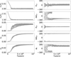 |
Fig. 18 Formation and evolution of the 1:2:3 resonant chain via convergent planetary migration. The left panels show the temporal evolutions of period ratios and eccentricities, and the critical angles are shown in the right panels. The planetary system is captured in symmetric configuration S6 firstly, subsequently evolves along the A6 family and finally librates around the asymmetric configuration. |
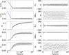 |
Fig. 19 Same as Fig. 18 but for a ‘joint two-body MMR’ case (see text). In the final resonance configuration, Δϖ12 and φ0 circulate while θ12, θ23, and Δϖ23 librate. The vertical lines in the left panels indicate two moments t1 = 1.2 Myr and t2 = 1.8 Myr. |
5.2 Other resonant chains
So far, our investigations have been on the 1:2:3 resonant chain. The consistence between the averaged Hamiltonian and the numerical simulations motivates us to extend our semi-analytical model to other resonant chains. As far as we know, previous works, for example, Morrison et al. (2020) and Kajtazi et al. (2023), mainly focus on the 1st order resonant chains with (k21 − k12 = k32 − k23 = 1). To show how our methods may work for general resonant chains, below we present our analyses on some other resonant chains. We also note that starting from circular orbits, the ACR solutions of a resonant chain may emerge as symmetric configurations with critical resonant angles being 0, π, or as asymmetric ones.
5.2.1 Cases starting from symmetric configuration
We will show two cases, a 2:3:5 resonant chain and a 3:5:7 resonant chain. The former is a resonant chain of mixed orders consisting of the 1st and 2nd order MMRs between adjacent planets, while the latter is a resonant chain with two second order MMRs. Although no exoplanetary system has been confirmed in these resonant configuration, we present these two examples to demonstrate the availability of methods introduced in this paper for higher-order resonances. Meanwhile the existence of such configuration but absence of such real systems also implies that the stability of such configuration is weak.
For the 2:3:5 resonant chain, we consider the fictitious planetary system with central star of mass M = 1 and three planets m1 = m2 = m3 = m = 10−6, and as before, the semi-major axis of m2 is set as a2 = 1 AU. Using the same technique we have applied to the 1:2:3 resonance chain, we obtain the symmetric and asymmetric ACR solutions and their stabilities for the 2:3:5 resonant chain. Following the definition of critical angles in Eq. (9), we define
![Mathematical equation: $\[\begin{cases}\theta_{12}=3 \lambda_2-2 \lambda_1-\varpi_1, & \Delta \varpi_{12}=\varpi_1-\varpi_2, \\ \theta_{23}=5 \lambda_3-3 \lambda_2-2 \varpi_2, & \Delta \varpi_{23}=\varpi_2-\varpi_3,\end{cases}\]$](/articles/aa/full_html/2024/07/aa49463-24/aa49463-24-eq59.png) (26)
(26)
and we find that the symmetric family with (θ12, Δϖ12, θ23, Δϖ23) = (0, π, π, π) is the unique stable ACR arising from the circular configuration. Along this family, the planets may evolve to the configuration of high eccentricities when the angular momentum G decreases. This stable symmetric family finally halts at (e1, e2, e3) = (0.311, 0.275, 0.294) where the planetary system may experience close encounters. Our detailed analyses on the dynamical maps reveal that all the regular motions we found in this 2:3:5 resonant chain are characterised by quasi-periodic libration around the ACR.
To investigate the formation and evolution of this resonant chain, we perform numerical simulations of the convergent migration and resonance capture again. The initial period ratio T2/T1 is uniformly distributed in the range [1.51, 1.53], and T3/T2 in [1.68, 1.71]. All planets’ initial orbits are assumed to be coplanar and circular, and the angles ϖi = 0, λi = 0. The migration timescales for three planets τa,1, τa,2, τa,3 are set as 0.3, 0.2, 0.1 Gyr, respectively, and the eccentricity damping time scale τe,i is set to satisfy κ = τa,i/τe,i = 100.
We find that all of 225 fictitious systems are captured into the 2:3:5 resonant chain and evolve along the stable symmetric family (θ12, Δϖ12, θ23, Δϖ23) = (0, π, π, π). Instead of plotting the evolutions of orbital elements and the resonant angles, we depict on eccentricities planes the migrating path along this ACR family in Fig. 20. It’s clear that this stable ACR family guides the migration of the planetary system. The evolution eventually stops at ![Mathematical equation: $\[\left(e_1^*, e_2^*, e_3^*\right)=(0.0460,0.0612,0.0122)\]$](/articles/aa/full_html/2024/07/aa49463-24/aa49463-24-eq60.png) in this example, but surely the final status depends on the migrating parameters. If all the torques on planets disappear at this moment, the system will oscillate around the stable ACR at
in this example, but surely the final status depends on the migrating parameters. If all the torques on planets disappear at this moment, the system will oscillate around the stable ACR at ![Mathematical equation: $\[\left(e_1^*, e_2^*, e_3^*\right)\]$](/articles/aa/full_html/2024/07/aa49463-24/aa49463-24-eq61.png) in the long term.
in the long term.
For the case of the 3:5:7 resonant chain, the critical angles are defined as in Eq. (9)
![Mathematical equation: $\[\begin{cases}\theta_{12}=5 \lambda_2-3 \lambda_1-2 \varpi_1, & \Delta \varpi_{12}=\varpi_1-\varpi_2, \\ \theta_{23}=7 \lambda_3-5 \lambda_2-2 \varpi_2, & \Delta \varpi_{23}=\varpi_2-\varpi_3,\end{cases}\]$](/articles/aa/full_html/2024/07/aa49463-24/aa49463-24-eq62.png) (27)
(27)
and the stable symmetric ACR of (θ12, Δϖ12, θ23, Δϖ23) = (π, π, π, π) was found to dominate the regular motion when the eccentricities are small. This symmetric ACR solution loses its stability at (e1, e2, e3) = (0.196, 0.238, 0.0845) and it bifurcates into two branches of asymmetric families in a similar way as in the 1:2:3 resonant chain. Along the asymmetric family, the eccentricities might finally attain (e1, e2, e3) = (0.267, 0.568, 0.617). Since both the 3:5 and 5:7 MMRs are relatively high order resonances, the resonant capture can be observed only if the migration is very slow. We show an example of the formation of 3:5:7 resonant chain in Fig. 21, where the migration timescales τa,1, τa,2, τa,3 for three planets are 5, 2, and 1 Gyr, respectively. In fact, if a faster migration rate is applied, most of the systems will skip the 3:5:7 resonance chain and fall into a more compact configuration. We note that such a phenomenon has been reported in Kajtazi et al. (2023).
To produce the 3:5:7 resonant chain as in Fig. 21, we started our simulations from initial (n1/n2, n2/n3) = (1.668, 1.402), which are very close to the nominal values in the resonant chain. And an eccentricity damping effect with κ = 100 was imposed in our simulations. The system evolves along the stable symmetric ACR (θ12, Δϖ12, θ23, Δϖ23) = (π, π, π, π) and the eccentricity damping effect finally halts the system around the configuration ![Mathematical equation: $\[\left(e_1^*, e_2^*, e_3^*\right)=(0.0272,0.0627,0.0356)\]$](/articles/aa/full_html/2024/07/aa49463-24/aa49463-24-eq63.png) .
.
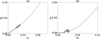 |
Fig. 20 Resonant capture and evolution of the 2:3:5 resonant chain on the eccentricities plane. The stable (θ12, Δϖ12, θ23, Δϖ23) = (0, π, π, π) ACR is indicated by blue dashed lines while the grey dots show the migrating path of the system evolving to higher eccentricities. |
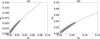 |
Fig. 21 Same as Fig. 20 but for the 3:5:7 resonant chain. The blue dashed lines indicate the location of the stable ACR of (θ12, Δϖ12, θ23, Δϖ23) = (π, π, π, π). |
5.2.2 Cases starting from asymmetric configuration
For all the aforementioned cases (1:2:3, 2:3:5, and 3:5:7 resonant chains), the stable ACR solutions arising from the circular configuration are always symmetric ones. As a result, the three-body Laplace angle φ0 is always librating around the symmetric value, 0 or π. In this sense, if the φ0 is found to librate around 0 or π, the system must be in such a resonant chain. However, this rule breaks for the 2:3:4 resonant chain. Siegel & Fabrycky (2021) find that the unreduced three-body critical angle 2φ0 (they adopt 2φ0 = 2λ1 + 4λ3 − 6λ2 instead of φ0) for the 2:3:4 resonant chain shift to asymmetric values ~ 162° and ~ 198°, instead of the symmetric value 2π.
Motivated by this interesting result, we apply our model to the 2:3:4 resonant chain with mass parameters M = 1, m1 = m2 = m3 = 10−5, similar to the ones in Siegel & Fabrycky (2021). The resonant angles are
![Mathematical equation: $\[\begin{cases}\theta_{12}=3 \lambda_2-2 \lambda_1-\varpi_1, & \Delta \varpi_{12}=\varpi_1-\varpi_2, \\ \theta_{23}=4 \lambda_3-3 \lambda_2-\varpi_2, & \Delta \varpi_{23}=\varpi_2-\varpi_3.\end{cases}\]$](/articles/aa/full_html/2024/07/aa49463-24/aa49463-24-eq64.png) (28)
(28)
Different from the 1:2:3 case, the final averaged Hamiltonian ![Mathematical equation: $\[\mathcal{H}\]$](/articles/aa/full_html/2024/07/aa49463-24/aa49463-24-eq65.png) for the 2:3:4 resonant chain is not 2π-periodically dependent on the angles (θ12, Δϖ12, θ23, Δϖ23). Following the procedure in Appendix A, we find that the degeneracy of these four resonant angles are (2, 2, 2, 1), respectively. Instead of the symmetric ACRs, we found two stable asymmetric ACRs in the near-circular configuration. We present these ACRs by black lines in Fig. 22. For better view, only one of the two asymmetric families is plotted in Fig. 22, the other family simply takes the same values in terms of (e1, e2, e3) and the symmetrically opposite values of the resonant angles.
for the 2:3:4 resonant chain is not 2π-periodically dependent on the angles (θ12, Δϖ12, θ23, Δϖ23). Following the procedure in Appendix A, we find that the degeneracy of these four resonant angles are (2, 2, 2, 1), respectively. Instead of the symmetric ACRs, we found two stable asymmetric ACRs in the near-circular configuration. We present these ACRs by black lines in Fig. 22. For better view, only one of the two asymmetric families is plotted in Fig. 22, the other family simply takes the same values in terms of (e1, e2, e3) and the symmetrically opposite values of the resonant angles.
Starting from circular orbits and initial period ratios T2/T1 uniformly in [1.51,1.53] and T3/T2 in [1.34,1.36], three planets m1, m2, m3 in 225 fictitious systems with different initial period ratios are forced to migrate with migration timescales τa,i = 1, 0.5, 0.2 Gyr, while the eccentricity damping effect satisfies κ = τa,i/τe,i = 50. All these systems are eventually captured into either one of the two asymmetric ACR families. And a typical example of resonant capture and evolution is overlaid on the stable ACRs in Fig. 22.
As shown in Figs. 22c, d, once the system reaches the 2:3:4 resonant chain just after the migration begins when the orbits are still near circular, the resonant angles are immediately locked into the asymmetric value (θ12, Δϖ12, θ23, Δϖ23) = (27.0°, 144.8°, 9.9°, 162.7°) and the Laplace angle librates around 2φ0 = 162.7° (Mod[360°]). The system evolves subsequently along the asymmetric ACR family and eventually librates around the ACR located at ![Mathematical equation: $\[\left(e_1^*, e_2^*, e_3^*\right)=(0.0357,0.0512,0.0265)\]$](/articles/aa/full_html/2024/07/aa49463-24/aa49463-24-eq66.png) and
and ![Mathematical equation: $\[\left(\theta_{12}^*, \Delta \varpi_{12}^*, \theta_{23}^*, \Delta \varpi_{23}^*\right)=\left(33.4^{\circ}, 138.4^{\circ}, 15.0^{\circ}, 160.0^{\circ}\right)\]$](/articles/aa/full_html/2024/07/aa49463-24/aa49463-24-eq67.png) .
.
Therefore, for the 2:3:4 resonant chain, our numerically averaged Hamiltonian successfully predicts the librating centres of resonant angles, as well as the adiabatic evolution induced by the convergent migration. In fact, starting from circular orbits, asymmetric ACR solutions are also found in the 3:4:6 and the 12:15:20 resonant chains (Siegel & Fabrycky 2021), and our calculations detected three and four stable ACR families starting from the circular configuration, respectively. For reference, we list in Table 2 the basic properties of the ACR solutions in some low-order three-planet resonant chains.
From Table 2, we see the number of stable ACR solutions is equal to the highest degeneracy number of the corresponding resonant angles. This number, and the symmetry properties (symmetric or asymmetric) of these stable ACR families, might depend not only on the resonant orders, but also on the degeneracies of the involved two-body MMRs. A general model for this question is still needed.
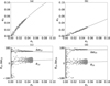 |
Fig. 22 Resonant capture and evolution of the 2:3:4 resonant chain. The black lines indicate the location of the asymmetric ACR solution arising from the circular configuration. The grey dots stand for the capture and evolution of planets by the resonant chain in the numerically simulated convergent migration. |
Properties of the ACR solutions in the low-order three-planet resonant chain.
5.3 Remarks on final resonant configurations
As we have shown above, starting from circular configuration (e1 = e2 = e3 = 0), the stable families of periodic orbits (ACR solutions, either symmetric or asymmetric) always exist in the resonant chains. These solutions guide the formation and adiabatic evolution of the resonant chains during the planetary migration. Depending on the migration parameters (τa,i, τe,i) and initial conditions, a triple-planet system finally attains different configurations of resonant chain, including the quasi-periodic motion around the ACR solutions and the joint two-body MMRs.
After the three planets have been trapped in a resonant chain, they may acquire high eccentricities as the system evolves along the path defined by the ACR solutions as the convergent migration continues. There are also some ACR solutions in the high eccentricity region that do not originate from the circular configuration (Voyatzis 2016). Since our methods of finding the ACR solutions work for arbitrary eccentricities, these high-eccentricity configurations can be calculated, but they cannot be attained through the adiabatic process from circular orbits as described above. Considering the fact that the typical eccentricities in the resonant chain are small (see e.g. Sun et al. 2017), we skip these configurations in this paper.
Another factor that can affect the final orbital configuration in a resonant chain is the planetary masses. For massive planets (e.g. Jupiter mass), the short-term perturbations will manifest their significances, and thus the formation and evolution of resonances in the system may not be smooth (adiabatic). One numerical example of the 1:2:4 resonant chain of massive planets can be found in Voyatzis (2016). The system can be captured into resonances through chaotic (irregular) processes and finally attain configurations of high eccentricities. Last but not least, in a compact planetary system, the tidal effect may modify the planets semimajor axes and eccentricities in an adiabatic way, thus it might play an important role in shaping the configuration of a resonant chain. As a matter of fact, the most well-known resonant chain, the literal ‘Laplace resonance’ in the three Jovian moons is believed to have formed through the tidal evolution (see e.g. Malhotra 1991).
6 Conclusion
In this paper, we generalise the semi-analytical model of MMR between two planets to the resonant chain in the triple-planet systems. By constructing and appropriately averaging the Hamiltonian that describes the dynamics of three planets in a resonant chain, we numerically computed the periodic orbits in the resonant chain. The periodic orbits in the resonance (also known as ACR solutions) are the stationary solutions to the averaged Hamiltonian equations and correspond to the extrema of the Hamiltonian function, which can be searched out numerically in the phase space.
Adopting the 1:2:3 resonant chain in the Kepler-51 system as an example, we calculated these ACR solutions and then analysed their stabilities by checking the topologies of the Hamiltonian on different representative planes. The stable symmetric ACRs we found are in good agreement with the stable symmetric periodic orbits obtained previously through the continuation method (Antoniadou & Voyatzis 2022). The symmetric ACR solutions lose their stabilities as the eccentricities increase, and they might bifurcate to asymmetric ACRs, which create stable configurations in the high-eccentricity region.
To investigate the orbital dynamics of the resonant chain near the stable ACRs, we constructed dynamical maps on the representative (e1, e2) plane and associate the orbital features with the Hamiltonian topology on the same plane. The dynamical maps show that the domain near the stable ACRs is always characterised by regular motion of quasi-periodic libration. The consistence between the topology and dynamical map simplifies the calculation of the stability of planetary systems in the resonant chain.
The behaviour of resonant angles in the resonant chain might be so complicated that we cannot always determine the resonance state simply by checking whether the corresponding critical angle is librating or not. In some cases, the short-term perturbations muddle the libration of resonance angles even when the system is dominated by the resonance. Thus, we calculated the deviation (χ2) of a resonant angle from a uniform distribution, and empirically defined the χ2 criterion to distinguish the resonance.
In the vicinity of the ACRs, we found two types of stable motion in the resonant chain. One is the periodic or quasi-periodic motion at or around the ACR solution, which is characterised by concurrent libration of the two-body resonant angles and the three-body Laplace angle. The other is the quasi-periodic motion, in which only the two-body resonant angles but not the Laplace angle librate. We denote the latter motion as joint two-body MMRs. Another difference between these two types of motion is that the centre (in terms of eccentricities and critical angles) of libration for the former is just the ACR solution while for the latter the ACR is not even ‘reached by the libration. According to our experiences, in both cases, the two-body MMRs between planet pairs are the essential mechanism that stabilises the planetary resonant chain, and the pure three-body resonance contributes little to the stability. Last but not least, we note that the two-body MMRs in a resonant chain are not the same as the usual two-body resonance that is isolated from other planets in a planetary system.
Just like the usual two-body MMR, the resonant chain could also be formed via the convergent migration of planets. Setting the initial conditions and migration velocities for each planet carefully, we verified the formation and evolution of the resonant chain. Starting from near circular orbits, the planets can be trapped to form the resonant chain. And all these systems are either in the quasi-periodic orbits around the ACR solution or in the joint two-body MMRs, as predicted by our model. As the migration continues, the system evolves to a high-eccentricity region along the ACR solutions.
In the high-eccentricity region, there exist some ACR solutions that do not arise from near circular orbits. These solutions can also be determined using the methods introduced in this paper, but these resonant configurations generally cannot be achieved through the convergent migration. In addition, such a resonant chain of high eccentricity has a relatively poor stability.
The configuration and stability of a resonant chain may be affected by the planetary mass. Not only do the locations of the ACRs change, but also the stability region shrinks as the individual planet mass increases. In fact, the more massive the planets are, the stronger the disturbances between planets. Thus the resonant chains, especially those compact ones, are more likely to occur in planetary systems of sub-Neptunes or even lighter planets.
Our methods introduced in this paper can be applied to any resonant chains. We have briefly shown our calculations of the ACR solutions and formation for the 2:3:5, 3:5:7, 2:3:4, 3:4:6, and 12:15:20 resonant chains. Diversified orbital configurations are found in different systems. Particularly, both symmetric ACR solutions (e.g. in the 1:2:3, 2:3:5, and 3:5:7 resonant chains) and asymmetric ones (e.g. in 2:3:4, 2:3:6, 3:4:6, and 12:15:20) emerge from circular orbits. Our methods can also be applied to longer resonant chains consisting of more than three planets. As an example, in Appendix B, we calculated the periodic solutions of the four-planet 3:4:6:8 resonant chain in Kepler-223, and show the resonant configurations as the function of scaled AMD δ.
Acknowledgements
This work has been supported by the National Key R&D Program of China (2019YFA0706601) and National Natural Science Foundation of China (NSFC, Grants No.12373081, No.12150009 & No.11933001). We also thank the supports from the science research grant from the China Manned Space Project with No. CMS-CSST-2021-B08.
Appendix A Degeneracy of the resonance
The literal expansion of perturbation part ![Mathematical equation: $\[\mathcal{H}\]$](/articles/aa/full_html/2024/07/aa49463-24/aa49463-24-eq68.png) 1 of the Hamiltonian in Eq. (7) takes the form
1 of the Hamiltonian in Eq. (7) takes the form
![Mathematical equation: $\[\begin{aligned}\mathcal{H}_1 & =\sum_{1 \leq i<j \leq n} \frac{p_i p_j}{M}-\mathcal{G} \frac{m_i m_j}{r_{i j}}=\sum_{1 \leq i<j \leq n} H_{1, i j}\left(\theta_{i j}, \Delta \varpi_{i j}, Q_{i j}\right) \\& =\sum_{1 \leq i<j \leq n} \sum_{l, m, k} H_{1, i j}^{l m k} \cos \left(l \theta_{i j}+m \Delta \varpi_{i j}+k Q_{i j}\right),\end{aligned}\]$](/articles/aa/full_html/2024/07/aa49463-24/aa49463-24-eq69.png) (A.1)
(A.1)
where l, m, k ∈ Z, θij = kjiλj − kijλi − (kji − kij)ϖi, Δϖij = ϖi − ϖj, Qij = λi − λj. After the numerically averaging process, terms with k ≠ 0 in Eq. (A.1) will not appear in the averaged Hamiltonian ![Mathematical equation: $\[\bar{\mathcal{H}}\]$](/articles/aa/full_html/2024/07/aa49463-24/aa49463-24-eq70.png) . Thus, the literal expansion of
. Thus, the literal expansion of ![Mathematical equation: $\[\bar{\mathcal{H}}_1\]$](/articles/aa/full_html/2024/07/aa49463-24/aa49463-24-eq71.png) 1 can be reduced to
1 can be reduced to
![Mathematical equation: $\[\begin{aligned}\bar{\mathcal{H}}_1 & =\sum_{1 \leq i<j \leq n} \frac{1}{T_{Q_{i j}}} \int_0^{T_{Q_{i j}}}\left(\frac{p_i p_j}{M}-\mathcal{G} \frac{m_i m_j}{r_{i j}}\right) \mathrm{d} Q_{i j} \\& =\sum_{1 \leq i<j \leq n} H_{1, i j}\left(\theta_{i j}, \Delta \varpi_{i j}\right) \\& =\sum_{1 \leq i<j \leq n} \sum_{l, m} H_{1, i j}^{l m} \cos \left(l \theta_{i j}+m \Delta \varpi_{i j}\right).\end{aligned}\]$](/articles/aa/full_html/2024/07/aa49463-24/aa49463-24-eq72.png) (A.2)
(A.2)
There are n(n − 1) resonant angles (θij, Δϖij), 1 ≤ i < j ≤ n appearing in the final expression at first glance. But in fact, these angles are linearly dependent. If we choose the two-body resonant angles between the adjacent planet pair θi,i+1, Δϖi,i+1 to characterise the configuration, the resonance angles between non-adjacent planets shall be linear combinations of angles θi,i+1, Δϖi,i+1 with the coefficients being fractions rather than integers. As a result, the Hamiltonian may not be 2π-periodic for all the resonant angles, e.g. the resonant configuration characterised by (θ12, Δϖ12, ⋯, θn−1,n, Δϖn−1,n) may not be identical to the one by (θ12 + 2π, Δϖ12, ⋯, θn−1,n, Δϖn−1,n). For instance, the resonant angles for the 2:3:4 resonant chain are
![Mathematical equation: $\[\begin{cases}\theta_{12}=3 \lambda_2-2 \lambda_1-\varpi_1, & \Delta \varpi_{12}=\varpi_1-\varpi_2, \\ \theta_{23}=4 \lambda_3-3 \lambda_2-\varpi_2, & \Delta \varpi_{23}=\varpi_2-\varpi_3.\end{cases}\]$](/articles/aa/full_html/2024/07/aa49463-24/aa49463-24-eq73.png) (A.3)
(A.3)
And the resonant angles between planets m1, m3
![Mathematical equation: $\[\theta_{13}=2 \lambda_3-\lambda_1-\varpi_1, \quad \Delta \varpi_{13}=\varpi_1-\varpi_3\]$](/articles/aa/full_html/2024/07/aa49463-24/aa49463-24-eq74.png) (A.4)
(A.4)
can be linearly expressed by θ12, Δϖ12, θ23, Δϖ23 as
![Mathematical equation: $\[\theta_{13}=\frac{1}{2}\left(\theta_{12}+\theta_{23}-\Delta \varpi_{12}\right), \quad \Delta \varpi_{13}=\Delta \sigma_{12}+\Delta \varpi_{23}.\]$](/articles/aa/full_html/2024/07/aa49463-24/aa49463-24-eq75.png) (A.5)
(A.5)
In this case, θ12, θ23, and Δϖ12 are not 2π-periodic angles, but 4π-periodic.
Generally, we define the degeneracy of an angle ϕ (ϕ stands for any one of θij, Δϖij) as the smallest positive integer q which satisfies the following condition:
![Mathematical equation: $\[\begin{aligned}& \bar{\mathcal{H}}_1\left(\theta_{12}, \cdots, \phi, \cdots, \theta_{n-1, n}, \Delta \varpi_{n-1, n}\right) \\& \quad=\bar{\mathcal{H}}_1\left(\theta_{12}, \cdots, \phi+2 q \pi, \cdots, \theta_{n-1, n}, \Delta \varpi_{n-1, n}\right).\end{aligned}\]$](/articles/aa/full_html/2024/07/aa49463-24/aa49463-24-eq76.png) (A.6)
(A.6)
Therefore, for the 2:3:4 resonant chain, the degeneracy of the angles (θ12, Δϖ12, θ23, Δϖ23) are (2, 2, 2, 1). The topology of the averaged Hamiltonian with e1 = e2 = e3 = 10−4 on angular plane is shown in Fig. A.1, in which the periodicity confirms the degeneracy of resonant angles. From the plots in Fig. A.1, we also note that no stable symmetric configuration exists for near circular orbit.
According to the form of averaged Hamiltonian, the asymmetric ACRs always appear in pair. If an ACR locates at (θ12, Δϖ12, ⋯, θn−1,n, Δϖn−1,n), one must find an ACR at (−θ12, −Δϖ12, ⋯, −θn−1,n, −Δϖn−1,n).
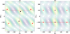 |
Fig. A.1 Topology of the averaged Hamiltonian for the 2:3:4 resonant chain on (a) the (θ12, Δϖ12) plane and (b) the (θ23, Δϖ23) plane. The solid black and red circles indicate the location of the stable and unstable ACRs, respectively. |
Appendix B Extension to four-planet resonant chain: Kepler-223 as an example
The methods introduced in this paper can be extended to resonant chains of more planets. As an example, we briefly present our analyses on the four-planet system Kepler-223, in which the orbital periods are close to T1: T2: T3: T4 = 3:4:6:8. The following resonant angles are adopted to characterise the resonant configuration.
![Mathematical equation: $\[\begin{cases}\theta_{12}=4 \lambda_2-3 \lambda_1-\varpi_1, & \Delta \varpi_{12}=\varpi_1-\varpi_2, \\ \theta_{23}=3 \lambda_3-2 \lambda_2-\varpi_2, & \Delta \varpi_{23}=\varpi_2-\varpi_3, \\ \theta_{34}=4 \lambda_4-3 \lambda_3-\varpi_3, & \Delta \varpi_{34}=\varpi_3-\varpi_4.\end{cases}\]$](/articles/aa/full_html/2024/07/aa49463-24/aa49463-24-eq77.png) (B.1)
(B.1)
After some algebra, we obtain the degeneracy of these resonant angles as (3, 3, 6, 2, 2, 1), which means that the searching for resonant configuration will be done in ![Mathematical equation: $\[\mathcal{T}\]$](/articles/aa/full_html/2024/07/aa49463-24/aa49463-24-eq78.png) 6 = [0, 6π] × [0, 6π] × [0, 12π] × [0, 4π] × [0, 4π] × [0, 2π]. The numerical averaging over the synodic angle Q reduces the final Hamiltonian to 6 DoF with two free parameters, the spacing parameter L and the total angular momentum G,
6 = [0, 6π] × [0, 6π] × [0, 12π] × [0, 4π] × [0, 4π] × [0, 2π]. The numerical averaging over the synodic angle Q reduces the final Hamiltonian to 6 DoF with two free parameters, the spacing parameter L and the total angular momentum G,
![Mathematical equation: $\[L=\sum_{i=1}^4 \frac{\Lambda_i}{k_i}, \quad G=\sum_{i=1}^4 \Lambda_i-\Gamma_i,\]$](/articles/aa/full_html/2024/07/aa49463-24/aa49463-24-eq79.png) (B.2)
(B.2)
where Λi and Γi are the Poincaré variables as in Eq. (8).
We only consider here the stable ACRs that correspond to libration in the resonance. Taking the mass parameters of Kepler-223 from Mills et al. (2016), and following the geometric method described in the main text, we found 6 (= 2 × 3) families of stable ACR. In Fig. B.1 we summarise the locations and configurations of these ACR families as the function of the scaled AMD, defined in the same way as Eq. (18), ![Mathematical equation: $\[\delta={\sum}_{i=1}^4 \Gamma_i / L\]$](/articles/aa/full_html/2024/07/aa49463-24/aa49463-24-eq80.png) . We also plot the Laplace angles φ123 = λ1 + λ3 − 2λ2, φ234 = λ2 + 2λ4 − 3λ3 for adjacent three planets. It’s worth noting that the six asymmetric solutions we obtained actually take only three configurations, and each configuration contains two branches that are symmetric with respect to each other. That’s why only three lines in each panel for eccentricities in Fig. B.1 can be seen.
. We also plot the Laplace angles φ123 = λ1 + λ3 − 2λ2, φ234 = λ2 + 2λ4 − 3λ3 for adjacent three planets. It’s worth noting that the six asymmetric solutions we obtained actually take only three configurations, and each configuration contains two branches that are symmetric with respect to each other. That’s why only three lines in each panel for eccentricities in Fig. B.1 can be seen.
Our results obtained from the averaged Hamiltonian are consistent with the analytical results (Delisle 2017). Since the analytical model in Delisle (2017) is truncated at the first order of eccentricity, it gives constant critical angles at the ACR solutions. However, our method provides more precise results. Some resonant angles θij, Δϖij are found to experience large variations along the ACR solutions, while the three-planet Laplace angle φ123 remains almost constant.
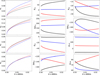 |
Fig. B.1 Locations and resonant configurations of six families of stable ACR for the four-planet resonant chain in Kepler-223. The variations of the eccentricities, the resonant angles, and the three-planet Laplace angles, are plotted against the scaled AMD (δ). Each family together with its symmetric opposite (see text) is represented by a specific colour in all panels. |
References
- Alves, A., Michtchenko, T. A., & Tadeu dos Santos, M. 2016, Celest. Mech. Dyn. Astron., 124, 311 [NASA ADS] [CrossRef] [Google Scholar]
- Antoniadou, K. I. 2016, Eur. Phys. J. Spec. Top., 225, 1001 [NASA ADS] [CrossRef] [Google Scholar]
- Antoniadou, K. I., & Voyatzis, G. 2016, MNRAS, 461, 3822 [NASA ADS] [CrossRef] [Google Scholar]
- Antoniadou, K. I., & Voyatzis, G. 2022, A&A, 661, A62 [NASA ADS] [CrossRef] [EDP Sciences] [Google Scholar]
- Beaugé, C., & Cerioni, M. 2022, Celest. Mech. Dyn. Astron., 134, 57 [CrossRef] [Google Scholar]
- Cerioni, M., & Beaugé, C. 2023, ApJ, 954, 57 [NASA ADS] [CrossRef] [Google Scholar]
- Cerioni, M., Beaugé, C., & Gallardo, T. 2022, MNRAS, 513, 541 [NASA ADS] [CrossRef] [Google Scholar]
- Charalambous, C., Martí, J. G., Beaugé, C., & Ramos, X. S. 2018, MNRAS, 477, 1414 [NASA ADS] [CrossRef] [Google Scholar]
- Christiansen, J. L., Crossfield, I. J., Barentsen, G., et al. 2018, AJ, 155, 57 [NASA ADS] [CrossRef] [Google Scholar]
- Delisle, J.-B. 2017, A&A, 605, A96 [NASA ADS] [CrossRef] [EDP Sciences] [Google Scholar]
- Delisle, J.-B., Correia, A., & Laskar, J. 2015, A&A, 579, A128 [NASA ADS] [CrossRef] [EDP Sciences] [Google Scholar]
- Gallardo, T. 2014, Icarus, 231, 273 [Google Scholar]
- Goldberg, M., Batygin, K., & Morbidelli, A. 2022, Icarus, 388, 115206 [NASA ADS] [CrossRef] [Google Scholar]
- Goździewski, K., & Migaszewski, C. 2020, ApJ, 902, L40 [CrossRef] [Google Scholar]
- Heller, R., Rodenbeck, K., & Hippke, M. 2019, A&A, 625, A31 [NASA ADS] [CrossRef] [EDP Sciences] [Google Scholar]
- Hénon, M. 2003, Generating Families in the Restricted Three-body Problem, 52 (Springer Science & Business Media) [Google Scholar]
- Hussain, N., & Tamayo, D. 2020, MNRAS, 491, 5258 [NASA ADS] [CrossRef] [Google Scholar]
- Jontof-Hutter, D., Ford, E. B., Rowe, J. F., et al. 2016, ApJ, 820, 39 [Google Scholar]
- Kajtazi, K., Petit, A. C., & Johansen, A. 2023, A&A, 669, A44 [NASA ADS] [CrossRef] [EDP Sciences] [Google Scholar]
- Laskar, J. 1991, in Predictability, Stability, and Chaos in N-Body Dynamical Systems (Springer), 93 [NASA ADS] [CrossRef] [Google Scholar]
- Laskar, J., & Petit, A. 2017, A&A, 605, A72 [NASA ADS] [CrossRef] [EDP Sciences] [Google Scholar]
- Leleu, A., Alibert, Y., Hara, N., et al. 2021, A&A, 649, A26 [NASA ADS] [CrossRef] [EDP Sciences] [Google Scholar]
- Lopez, T., Barros, S., Santerne, A., et al. 2019, A&A, 631, A90 [NASA ADS] [CrossRef] [EDP Sciences] [Google Scholar]
- MacDonald, M. G., & Dawson, R. I. 2018, AJ, 156, 228 [Google Scholar]
- MacDonald, M. G., Shakespeare, C. J., & Ragozzine, D. 2021, AJ, 162, 114 [NASA ADS] [CrossRef] [Google Scholar]
- MacDonald, M. G., Feil, L., Quinn, T., & Rice, D. 2022, AJ, 163, 162 [NASA ADS] [CrossRef] [Google Scholar]
- Malhotra, R. 1991, Icarus, 94, 399 [NASA ADS] [CrossRef] [Google Scholar]
- Masuda, K. 2014, ApJ, 783, 53 [Google Scholar]
- Michtchenko, T., Beaugé, C., & Ferraz-Mello, S. 2006, Celest. Mech. Dyn. Astron., 94, 411 [NASA ADS] [CrossRef] [Google Scholar]
- Michtchenko, T., Beaugé, C., & Ferraz-Mello, S. 2008, MNRAS, 387, 747 [NASA ADS] [CrossRef] [Google Scholar]
- Mills, S. M., Fabrycky, D. C., Migaszewski, C., et al. 2016, Nature, 533, 509 [Google Scholar]
- Morrison, S. J., Dawson, R. I., & MacDonald, M. 2020, ApJ, 904, 157 [NASA ADS] [CrossRef] [Google Scholar]
- Murray, C. D., & Dermott, S. F. 2000, Solar System Dynamics (Cambridge University Press) [Google Scholar]
- Petit, A. C. 2021, Celest. Mech. Dyn. Astron., 133, 1 [NASA ADS] [CrossRef] [Google Scholar]
- Petit, A. C., Laskar, J., & Boué, G. 2017, A&A, 607, A35 [NASA ADS] [CrossRef] [EDP Sciences] [Google Scholar]
- Petit, A., Pichierri, G., Davies, M. B., & Johansen, A. 2020, A&A, 641, A176 [NASA ADS] [CrossRef] [EDP Sciences] [Google Scholar]
- Pichierri, G., & Morbidelli, A. 2020, MNRAS, 494, 4950 [Google Scholar]
- Pichierri, G., Batygin, K., & Morbidelli, A. 2019, A&A, 625, A7 [NASA ADS] [CrossRef] [EDP Sciences] [Google Scholar]
- Press, W. H., Teukolsky, S. A., Vetterling, W. T., & Flannery, B. P. 1996, Numerical Recipes in Fortran 90 the Art of Parallel Scientific Computing (Cambridge University Press) [Google Scholar]
- Ramos, X. S., Correa-Otto, J. A., & Beauge, C. 2015, Celest. Mech. Dyn. Astron., 123, 453 [NASA ADS] [CrossRef] [Google Scholar]
- Rath, J., Hadden, S., & Lithwick, Y. 2022, ApJ, 932, 61 [NASA ADS] [CrossRef] [Google Scholar]
- Siegel, J. C., & Fabrycky, D. 2021, AJ, 161, 290 [NASA ADS] [CrossRef] [Google Scholar]
- Sun, Z., Ji, J., Wang, S., & Jin, S. 2017, MNRAS, 467, 619 [NASA ADS] [CrossRef] [Google Scholar]
- Voyatzis, G. 2008, ApJ, 675, 802 [Google Scholar]
- Voyatzis, G. 2016, Eur. Phys. J. Spec. Top., 225 [Google Scholar]
- Voyatzis, G., Kotoulas, T., & Hadjidemetriou, J. 2009, MNRAS, 395, 2147 [NASA ADS] [CrossRef] [Google Scholar]
- Wong, K. H., & Lee, M. H. 2024, AJ, 167, 112 [NASA ADS] [CrossRef] [Google Scholar]
All Tables
Critical angles (resonant angles, longitudes of pericentre ϖi, and mean anomalies Mi) of different symmetric resonant configurations.
All Figures
|
Fig. 1 Topology of the Hamiltonian on different representative planes, (a) The topology on period ratio plane (n1/n2, n2/n3) with fixed eccentricities. (b) The topology on eccentricity plane (e1,e2). The stationary solution located at (n1/n2, n2/n3) = (2, 1.5) and (e1, e2, e3) = (0.00458, 0.00938, 0.00564) is marked by a red dot on both panels. The corresponding critical angles are (θ12, Δϖ12, θ23, Δϖ23) = (π, 0, π, π). The colour indicates the value of Hamiltonian, light yellow for high and dark blue for low. The same colour code is adopted in all figures in this paper, unless otherwise stated. |
| In the text | |
|
Fig. 2 Different topologies on the (e1, e2) plane for different symmetric configurations (a) (θ12, Δϖ12, θ23, Δϖ23) = (0, π, 0, π) and (b) (π, π, 0, 0). The local extrema are (e1, e2, e3) = (0.119,0.1352,0.119) (red solid circle) and (0.300, 0.0662, 0.0671) (red cross), respectively. |
| In the text | |
|
Fig. 3 Topology on representative angular planes. The eccentricities of the symmetric ACR are (e1, e2, e3) = (0.00458, 0.00938, 0.00564). (a) Hamiltonian level curves on (θ12, Δϖ12) plane with (θ23, Δϖ23) fixed to (π, π), the saddle-like point at (θ12, Δϖ12) = (π, 0) is marked by a red cross. (b) Topology on (θ23, Δϖ23) plane with (θ12, Δϖ12) fixed to (π, 0). The node-like point at (θ23, Δϖ23) = (π, π) is marked by a red dot. In addition, the stable symmetric configuration (θ12, Δϖ12, θ23, Δϖ23) = (0, π, 0, π) is shown as blue dots. |
| In the text | |
|
Fig. 4 Symmetric ACR families S2, S3, S5, and S6 in the 1:2:3 resonant chain for small-eccentricity configurations on (a) the (e1 cos θ1, e2 cos θ2) plane and (b) the (e2 cos θ2, e3 cos θ3) plane. The stable symmetric ACRs are in blue while the unstable ones in red. The notations of the families are the same as in Antoniadou & Voyatzis (2022), and the resonant angles of different configurations are presented in Table 1. |
| In the text | |
|
Fig. 5 Topology on representative angular planes for symmetric ACR S6 located at (e1e2,e3) = (0.0569, 0.0846, 0.0531). (a) Topology on (θ12, Δϖ12) plane with fixed (θ23, Δϖ23) = (0, π). The saddle-like point at (θ12, Δϖ12) = (0, π) marked by a cross indicates the instability of this solution, while two asymmetric ACRs bifurcated from this unstable symmetric one are indicated by black dots. (b) The topology on (θ23, Δϖ23) plane with (θ12, Δϖ12) fixed to (0, π). The node-like point at (θ23, Δϖ23) = (0, π) is marked by a pink dot. |
| In the text | |
|
Fig. 6 Locations and resonant configurations of the symmetric ACR family (S6) and the asymmetric ACR family (A6). In the upper two panels (a) and (b), the stable symmetric, unstable symmetric, and stable asymmetric ACRs are indicated by blue solid, red solid, and black dashed lines, respectively. Three solid circles on these lines indicate the initial conditions that will be analysed in detail later (see text). The lower two panels (c) and (d) show the evolutions of resonant angles along the asymmetric ACR as the function of δ (scaled AMD, see text). The resonant angles θ12, θ23 and the secular angles Δϖ12, Δϖ23 are labelled by the corresponding lines. |
| In the text | |
|
Fig. 7 Law of structure for the 1:2:3 resonant chain. The left (right) column of panels show the relation between the mean motion ratio n1/n2 (n2/n3) and the eccentricities (e1, e2, e3 from top to bottom). Blue lines are for the stable symmetric ACR families (S6) while the black lines for the stable asymmetric family (A6). On each panel, the lowest line is for the planets in the Kepler-51 system, while the middle and the top lines are for the cases of 10 and 100 times more massive planets, respectively (see text). The critical points, at which the S6 family becomes unstable and the asymmetric solution appears, are denoted by red crosses. |
| In the text | |
|
Fig. 8 Variation of the Hamiltonian in two synodic periods |
| In the text | |
|
Fig. 9 χ2 map for the standard pendulum model, (a) Phase structure (energy level) on (φ, pφ) plane. The broad red curve marks the separatrix between the libration and circulation region, (b) χ2 value in logarithm indicated by colour. |
| In the text | |
|
Fig. 10 Topology (contour line) and dynamical map (colour map) on the (e1, e2) plane for Case A, with constants L and G determined by the initial condition on the stable ACR solution (e1, e2, e3, θ12, Δϖ12, θ23, Δϖ23) = (0.0124, 0.0237, 0.0128, 0, π, 0, π), which is indicated by a red dot on all maps. The eccentricity variations Δei are used as the stability indicator as labelled in each panel. |
| In the text | |
|
Fig. 11 Resonant structure indicated by χ2 on the (e1, e2) plane for Case A. Four panels are for the two-body MMRs between (a) m1 and m2, (b) m2 and m3, (c) m1 and m3, and (d) the three-planet Laplace resonance with resonant angle φ0. The large value of χ2 (light colour) indicates that the resonant angle is in libration, while the small χ2 (dark tones) indicates circulation. The narrow strip-like structure indicated by a black arrow in (a) divides the map into two parts, namely Region 1 and Region 2. Moreover, another narrow strip (indicated by the red arrow) can be seen in Region 2. |
| In the text | |
|
Fig. 12 Typical behaviour of the orbits in Region 1 (Fig. 11a). The temporal variations of n1/n2, n2/n3, e1, e2, e3 are in left panels, while right panels are for resonant angles θ12, Δϖ12, θ23, Δϖ23, φ0. The orbits are librating quasi-periodically around the stable symmetric ACR solution S6. The eccentricities of S6 are indicated by horizontal dashed lines. |
| In the text | |
|
Fig. 14 Same as Fig. 10 but for Case B. The constants L and G are determined by the initial condition on the stable asymmetric ACR solution (black solid circle in Fig. 6). (a) Around the unstable symmetric ACR solution with the same L, G. The corresponding eccentricities e1, e2, e3 are 0.0569, 0.0846, 0.0531 (red solid circle in Fig. 6). (b) Around the stable asymmetric ACR solution. The colour in both panels indicates the value of max(Δe). |
| In the text | |
|
Fig. 15 Horseshoe-like orbit near the unstable symmetric ACR. The unstable symmetric ACR and the stable asymmetric ACRs are indicated by the red and black horizontal lines, respectively. |
| In the text | |
|
Fig. 16 Same as Fig. 11 but for Case B. The map is divided into two parts (Region 1 and Region 2) by a stripe-like structure of relatively smaller χ2 value, as indicated by the arrow in panel a. |
| In the text | |
|
Fig. 17 Same as Fig. 13 but the initial conditions are from the high eccentricity region of Fig. 14 (see text). |
| In the text | |
|
Fig. 18 Formation and evolution of the 1:2:3 resonant chain via convergent planetary migration. The left panels show the temporal evolutions of period ratios and eccentricities, and the critical angles are shown in the right panels. The planetary system is captured in symmetric configuration S6 firstly, subsequently evolves along the A6 family and finally librates around the asymmetric configuration. |
| In the text | |
|
Fig. 19 Same as Fig. 18 but for a ‘joint two-body MMR’ case (see text). In the final resonance configuration, Δϖ12 and φ0 circulate while θ12, θ23, and Δϖ23 librate. The vertical lines in the left panels indicate two moments t1 = 1.2 Myr and t2 = 1.8 Myr. |
| In the text | |
|
Fig. 20 Resonant capture and evolution of the 2:3:5 resonant chain on the eccentricities plane. The stable (θ12, Δϖ12, θ23, Δϖ23) = (0, π, π, π) ACR is indicated by blue dashed lines while the grey dots show the migrating path of the system evolving to higher eccentricities. |
| In the text | |
|
Fig. 21 Same as Fig. 20 but for the 3:5:7 resonant chain. The blue dashed lines indicate the location of the stable ACR of (θ12, Δϖ12, θ23, Δϖ23) = (π, π, π, π). |
| In the text | |
|
Fig. 22 Resonant capture and evolution of the 2:3:4 resonant chain. The black lines indicate the location of the asymmetric ACR solution arising from the circular configuration. The grey dots stand for the capture and evolution of planets by the resonant chain in the numerically simulated convergent migration. |
| In the text | |
|
Fig. A.1 Topology of the averaged Hamiltonian for the 2:3:4 resonant chain on (a) the (θ12, Δϖ12) plane and (b) the (θ23, Δϖ23) plane. The solid black and red circles indicate the location of the stable and unstable ACRs, respectively. |
| In the text | |
|
Fig. B.1 Locations and resonant configurations of six families of stable ACR for the four-planet resonant chain in Kepler-223. The variations of the eccentricities, the resonant angles, and the three-planet Laplace angles, are plotted against the scaled AMD (δ). Each family together with its symmetric opposite (see text) is represented by a specific colour in all panels. |
| In the text | |
Current usage metrics show cumulative count of Article Views (full-text article views including HTML views, PDF and ePub downloads, according to the available data) and Abstracts Views on Vision4Press platform.
Data correspond to usage on the plateform after 2015. The current usage metrics is available 48-96 hours after online publication and is updated daily on week days.
Initial download of the metrics may take a while.