| Issue |
A&A
Volume 687, July 2024
|
|
|---|---|---|
| Article Number | A287 | |
| Number of page(s) | 10 | |
| Section | Extragalactic astronomy | |
| DOI | https://doi.org/10.1051/0004-6361/202449286 | |
| Published online | 22 July 2024 | |
A high-resolution radio morphology and polarization of the kiloparsec-scale X-ray jet of PKS 1127−145
1
INAF – Istituto di Radioastronomia, Via P. Gobetti 101, 40129 Bologna, Italy
e-mail: This email address is being protected from spambots. You need JavaScript enabled to view it.
2
Harvard Smithsonian Center for Astrophysics, 60 Garden St, Cambridge, MA 02138, USA
Received:
19
January
2024
Accepted:
1
May
2024
Abstract
We report on new multifrequency Very Large Array (VLA) radio observations and Chandra X-ray observations of a radio-loud quasar with a ∼300 kpc-long jet, PKS 1127−145, during a flaring event detected in γ-rays by the Fermi Large Area Telescope in December 2020. The high angular resolution of the new radio images allows us to disentangle for the first time the kiloparsec-scale inner jet from the core contribution. The inner radio jet, up to 15 kpc from the core, is highly polarized (33 percent) and the magnetic field is parallel to the jet axis. At about 18 arcsecs from the core, the jet slightly bends and we observe a re-brightening of the radio emission and a 90-degree rotation of the magnetic field, likely highlighting the presence of a shock that is compressing the magnetic field to a plane perpendicular to the jet axis, where efficient particle acceleration takes place. At the same position, the X-ray emission fades, suggesting a deceleration of the bulk velocity of the jet after the bend. A change in velocity and collimation of the jet is supported by the widening of the jet profile and the detection of a limb-brightened structure connecting the bending region with the jet termination. The limb-brightened structure might indicate the coexistence of both longitudinal and transverse velocity gradients at the jet bending. There is no evidence of significant brightening of the kiloparsec-scale jet in the radio or X-ray band during the γ-ray flare. The X-ray flux, F2 − 10 keV = (6.24 ± 0.57)×10−12 ergs s−1 cm−2, measured by Chandra from the quasar core is consistent with the flux measured by the X-ray Telescope on board the Neil Gehrels Swift Observatory after the high-energy flare. Our results indicate that the γ-ray flaring region is located within the VLA source core.
Key words: polarization / radiation mechanisms: non-thermal / techniques: interferometric / X-rays: general / quasars: individual: PKS 1127-145
© The Authors 2024
 Open Access article, published by EDP Sciences, under the terms of the Creative Commons Attribution License (https://creativecommons.org/licenses/by/4.0), which permits unrestricted use, distribution, and reproduction in any medium, provided the original work is properly cited.
This article is published in open access under the Subscribe to Open model. This email address is being protected from spambots. You need JavaScript enabled to view it. to support open access publication.
1. Introduction
The extragalactic γ-ray sky is dominated by blazars. The emission of this class of active galactic nuclei (AGN) comes mainly from the relativistic jet that is aligned close with our line of sight. As a consequence, the luminosity is augmented by Doppler boosting and beaming effects and variability is observed across the electromagnetic spectrum. Among the extragalactic γ-ray sources detected by the Large Area Telescope (LAT) on board the Fermi Gamma-ray Space Telescope satellite (hereafter Fermi), flat spectrum radio quasars (FSRQs) show the most dramatic flaring events. Their γ-ray flux may increase by more than an order of magnitude above the average level, with a doubling time of a few hours or even less (e.g., Abdo et al. 2011; Hayashida et al. 2015; D’Ammando et al. 2019).
Despite decades of studies, many aspects of the high-energy emission from AGN are still elusive. Among them, the location of the high-energy emitting region and the main radiative processes at work have been investigated intensively by multiband (and recently multi-messenger) observations. The detection of a (sub-)hour variability by Fermi-LAT of some FSRQs suggests a location between the broad line region (BLR) and the molecular torus (e.g., Abdo et al. 2011; Hayashida et al. 2015; Ackermann et al. 2016; Acharyya et al. 2021). On the other hand, Costamante et al. (2018) could not find significant evidence of cutoff signatures at high energies compatible with γ − γ interactions with BLR photons in the γ-ray spectra of a sample of FSRQs, suggesting that the γ-ray emitting region is far beyond the BLR. Very long baseline interferometry (VLBI) observations point out the appearance of superluminal jet components close in time to some γ-ray flares, indicating that the radio core is the locus of high-energy emission, a few pc from the central engine (e.g., Marscher et al. 2010; Agudo et al. 2011; Orienti et al. 2013; Jorstad et al. 2017).
Not all the high-energy flares originate in the same region, even when the same source is considered (see, e.g., Marscher et al. 2008, 2010; Orienti et al. 2013). A remarkable example is the radio galaxy M 87. High-resolution radio and X-ray observations found the jet knot HST-1 at 120 pc from the AGN to be the locus of the high-energy emission observed in 2005 (Cheung et al. 2007; Harris et al. 2009). The high activity state observed in 2012 originated at the source core, however, whereas HST-1 remained quiescent (Hada et al. 2014). Another example is the X-ray flaring activity observed in the extended jet of Pictor A that originated at about 48 arcsec (∼33 kpc) from the core, indicating that variability can be observed in the outer regions of relativistic jets (Marshall et al. 2010; Hardcastle et al. 2016).
X-ray variability in kiloparsec-scale jets and hotspots on timescales of a few months to years does not seem to be so uncommon (Meyer et al. 2023). Such relatively short timescales challenge a simple model of inverse Compton (IC) scattering of the cosmic microwave background (CMB) photons, and favor synchrotron emission from a second highly energetic population of relativistic electrons in compact (parsec-scale size) regions (e.g., Hardcastle et al. 2004; Tingay et al. 2008; Hardcastle et al. 2016; Migliori et al. 2020; Meyer et al. 2023). The IC-CMB model is called into question by other observational evidence, like the detection of kiloparsec-scale displacement between X-ray and radio emission in several knots and hotspots (e.g., Hardcastle et al. 2007; Mingo et al. 2017; Orienti et al. 2020a; Migliori et al. 2020; Reddy et al. 2023). However, it should be kept in mind that high-redshift jets may be different from those at low and intermediate redshift (e.g., McKeough et al. 2016; Ighina et al. 2022).
Not many AGN have relativistic jets that can be imaged on an arcsecond scale in X-rays. Moreover, only a handful of them are γ-ray emitters. Multiwavelength studies of these jets are crucial for investigating particle acceleration and emission mechanisms far away from the central engine.
PKS 1127−145, at z = 1.187 (Drinkwater et al. 1997), is one of the few γ-ray-emitting FSRQs with a prominent X-ray jet extending for ∼30″(Siemiginowska et al. 2002). This is one of the longest jets observed so far in X-rays. It was discovered in the first observation of PKS 1127−145 with the Chandra X-ray Observatory (hereafter Chandra). Three main knots are detected in X-rays along the inner part of the jet, whereas the radio emission peaks at the two outer knots associated with weak X-ray emission. The misalignment between radio and X-ray emission challenges our understanding of the jet structure and dominant radiation mechanism at the origin of the high-energy emission (Siemiginowska et al. 2002, 2007).
Fermi-LAT observed enhanced γ-ray activity from PKS 1127−145 in December 2020, reaching a daily γ-ray flux (E > 100 MeV) of (1.6 ± 0.3) × 10−6 photons cm−2 s−1 on December 10 (Angioni 2020), corresponding to a flux increase by a factor of about 50 relative to the value reported in the fourth Fermi-LAT source catalogue (Abdollahi et al. 2020). That was the first strong γ-ray flaring activity observed from this source in the Fermi era. Follow-up Swift-XRT observations on December 13 found that the X-ray flux of the source increased as well, reaching the highest X-ray flux observed by Swift-XRT so far (D’Ammando 2020a), suggesting a physical connection between the γ-ray and X-ray radiation processes. The subsequent Swift-XRT observations performed on December 15 and 17 confirmed that the X-ray flare was continuing (D’Ammando 2020b). However, the resolution of Swift-XRT is not adequate to spatially resolve the X-ray emission and locate the flaring region.
In this paper, we present results on new Chandra X-ray and Jansky Very Large Array (VLA) radio observations of PKS 1127−145 performed just after the γ-ray flaring event. These observations aim to investigate the jet structure and the location of the X-ray flaring region. Full-polarization radio data obtained with the VLA in A-configuration enable us to study for the first time the magnetic field structure with high (sub-arcsecond) angular resolution along the kiloparsec-scale jet of PKS 1127−145.
This paper is organized as follows: Sect. 2 describes the setting of the observations. Results on the kiloparsec-scale jet morphology in radio and X-rays are presented in Sect. 3 and discussed in Sect. 4. We draw our conclusions in Sect. 5.
Throughout this paper, we assume the following cosmology: H0 = 70 km s−1 Mpc−1, ΩM = 0.27, and ΩΛ = 0.73, in a flat Universe. At the redshift of the source, z = 1.187, 1 arcsec corresponds to 8.4 kpc (Wright 2006). The spectral index is defined as S(ν) ∝ ν−α. The position angle (PA) is measured from north to east, where north is up and east is left.
2. Observations
2.1. Very Large Array observations and data analysis
We were awarded 4.5 hr of Director’s Discretionary Time (DDT) at the VLA (project code VLA/20B-460) to observe PKS 1127−145 after the detection of a flaring state in γ rays (Angioni 2020). The VLA observations were performed on January 7, 2021 in the L (1–2 GHz), C (4–8 GHz), and X (8–12 GHz) bands in full polarization mode when the array was in A configuration. The on-source observing time was about 45 min in the L and C bands, and 70 min in the X band, spread into several scans and cycling through frequencies in order to improve the (u,v) coverage. The source 3C 286 was used as the primary calibrator, band pass calibrator, and electric vector position angle (EVPA) calibrator, while the unpolarized source OQ 208 was observed as the D-term calibrator.
The calibration was performed using Common Astronomical Software Applications (CASA) version 5.4.1 (McMullin et al. 2007), following the standard procedure for VLA data. Data were inspected and Hanning smoothed to reduce Gibbs ringing produced by strong radio frequency interference (RFI) present in some spectral windows, mainly in the L and C bands. After an initial flagging on bad data, we calibrated the datasets. We checked for antenna position corrections and ionospheric total electron content corrections. We set the flux density model for 3C 286 (no polarization model is set at this stage) using the Perley & Butler (2017) scale. We then performed an initial delay and bandpass calibration using 3C 286 before running a second flagging of RFI (setting “RFLAG” in the CASA task FLAGDATA). An initial gain calibration (both phase and amplitude) was performed. After applying the initial calibration to the data, we did a further RFI flagging. Then we performed the entire calibration again on the flagged data (delay, bandpass, and gain calibration).
At this point, we performed the polarization calibration. First, we set the polarization model for 3C 2861. Then, we solved for the cross-hand delays for 3C 286, before determining the D-terms for the unpolarized and unresolved calibrator OQ 208. Last, the polarization angle was calibrated, making use of 3C 286.
Errors on the amplitude calibration, σcal, were estimated by checking the scatter of amplitude gain factors, and turned out to be about 3 percent in all bands, in agreement with the errors reported in Perley & Butler (2017). Errors on the polarization angle are about 3–5 deg.
After the a priori calibration, we produced images using the CASA task tclean with multi-term multifrequency synthesis deconvolution (nterms=2), Briggs weightings, and robust = 0.5. Before creating the final images we performed a few phase-only self-calibration iterations, decreasing the solution intervals from 60 seconds to 10 seconds, followed by a single amplitude self-calibration with a solution interval of the scan length (see e.g., Cornwell & Fomalont 1999).
In addition to the total intensity images, we produced polarization intensity and polarization angle maps, combining images in Stokes Q and U using the CASA task immath. Pixels with values less than three times the rms measured on the input images were masked.
The restoring beam of the final images is 1.78 × 1.11 arcsec2 with a major axis PA of 17° at 1.5 GHz, 0.47 × 0.29 arcsec2 with PA 22° at 6 GHz, and 0.28 × 0.17 arcsec2 with PA 20° at 10 GHz.
We measured the flux density of the unresolved components using the CASA task imfit, which performs a two-dimensional Gaussian fit on the image plane. For resolved components and to estimate the total flux density, we used the task viewer, which extracts the flux density on a selected polygonal area on the image plane. Flux densities are reported in Table 1. The polarized flux density was measured in the same region as the one considered for total intensity measurements and is reported in Table 2, together with the EVPA.
VLA flux density of PKS 1127−145.
Polarization information.
Errors on the total intensity and polarized flux densities were estimated with  , where σcal is the error on the amplitude calibration, and σrms is the 1-σ noise level of the rms measured on the image plane. The latter contribution depends on the area of the selected region used for extracting the flux density, θsource, as
  , where θbeam is the area of the Gaussian restoring beam.
Depending on the position on the image of the component considered, the rms is measured either far from or close to the core component. The off-source noise level of the final images is 0.1 mJy beam−1, 0.025 mJy beam−1, and 0.015 mJy beam−1 in the L, C, and X bands, respectively. Imaging artifacts are present close to the core component, and the rms is higher in that area. This is likely due to the combination of the bright core, the low declination of the source, and the relatively short observing time. To improve the signal-to-noise ratio (S/N) we created a dataset in which we subtracted the model visibility data of the bright core from the corrected visibility data with the CASA task uvsub, leaving only the residuals. However, not all the artifacts could be removed and the rms did not improve significantly.
Fits files of the final images were imported into the Astronomical Image Processing System (AIPS), where contour images were produced with the KNTR task. The final images are shown in Fig. 1.
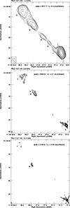 |
Fig. 1. Total intensity images of PKS 1127−145 at 1.5 GHz (top), 6 GHz (middle), and 10 GHz (bottom). The first contour is 0.6, 0.1, and 0.075 mJy beam−1 at 1.5, 6, and 10 GHz, respectively, and corresponds to three times the rms measured on the image plane close to the center. Contours are drawn at [−1, 1, 1.4, 2, 2.8, 4, 5.6, 8, 16, 32, 64,...] times the first contour. The restoring beam is plotted in the bottom left corner of each image. |
2.2. Chandra observations and data analysis
The Chandra DDT observation of PKS 1127−145 was performed on January 1, 2021 during the flaring events detected by Fermi and Swift. Our goal was to identify the X-ray site of the flare and check if the activity could be located outside the quasar core. The Chandra point spread function (PSF) allows for the best angular resolution X-ray images available today. Here, we present this new observation together with the archival data in order to inspect any variability in the jet.
During the course of the mission, Chandra observed PKS 1127−145 three times (see Table 3) using the ACIS-S3 detector with the target located at the aimpoint on the back-illuminated charge coupled device (CCD). The quasar is bright and in order to limit the CCD pileup all the observations were taken with 1/8 subarray readout. The data mode was set to VFAINT2 in the first two observations, which typically improves the identification of background events. The FAINT mode was used in the most recent observation. The first two observations were obtained early in the mission with a good detector response across all the energies, from 0.3–8 keV. However, the most recent observation performed in January 2021 had a degraded sensitivity due to the ACIS-S contamination buildup, which significantly reduced the number of counts in the soft energies; that is, below 1 keV.
Chandra observations.
We used CIAO version 4.15 software (Fruscione et al. 2006) for data analysis and Sherpa for fitting and modeling (Freeman et al. 2001; Refsdal et al. 2011). We reprocessed all three observations using the chandra_repro tool and applied the recent calibration products available in the CALDB v.4.10.4.
The standard aspect reconstruction shows a relatively large offset of about 1″ between the first two observations (ObsID 866, 5708) and the most recent one (ObsID 24911). We adjusted observations 866 and 24911 to match the coordinates of the longest one, 5708, and merged the three observations to obtain the best available Chandra image of the source. The images from individual observations are shown in Fig. 2 and the final merged image is shown in Fig. 3. The quasar is bright and the ACIS-S readout streaks are visible in the image presented in Fig. 2, as we did not remove them at this stage. We note that the streak is much fainter in the most recent observation with the shorter exposure and degraded soft energy response.
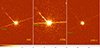 |
Fig. 2. ACIS-S 0.5-7 keV image showing the total number of counts per pixel obtained in each Chandra observation. The Chandra ObsID number is indicated in the bottom right corner of each panel, from left to right: 866, 5708, and 24911. The image pixels are the native ACIS-S pixel size of 0.492″. The image is displayed on a logarithmic scale with the color bar scale indicating the number of counts per pixel. In addition to the jet, the readout streak (labeled green) is visible with different angles dependent on the Chandra roll angle during the observation. |
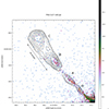 |
Fig. 3. ACIS-S 0.5–7 keV mosaic image binned into 0.246″ pixels (0.5 bin scale). The color bar shows the number of counts per pixel. The black contours are from the 1.6 GHz L-band VLA map starting at 0.45 mJy beam−1 and increasing by |

The jet of PKS 1127−145 is quite prominent and the outermost structure can be analyzed in relation to the radio emission, including polarization present in the outer knots. In addition, we performed the analysis of the innermost structures in the vicinity of a jet bend.
3. Results
In this paper, we follow the component nomenclature used in Siemiginowska et al. (2002) and Siemiginowska et al. (2007). The main knots, A, B, and C, are located ∼12″, 18″, and 27″ from the core, respectively. Two additional brightenings, labeled I and O, are located between the core and knot A (Fig. 1).
The flux densities in the L band of the main knots are consistent with the values reported in Siemiginowska et al. (2007). The lower values in the C and X bands are likely related to different characteristics of the observations. The datasets presented in Siemiginowska et al. (2002) and Siemiginowska et al. (2007) were obtained with a longer observing time and a more compact VLA configuration that is more effective at picking up diffuse emission than our observations.
3.1. The 2-arcsec inner jet structure
The new VLA radio observations allow for a detailed analysis of the inner 2-arcsec jet structure3, unlike earlier VLA observations, which did not have a sufficient resolution to disentangle it from the core (Siemiginowska et al. 2007). At 1.5 GHz the inner jet (labeled I in Fig. 1) is slightly resolved and is connected to the outer part of the jet by a low-surface brightness emission that bridges knots O and A. At 6 and 10 GHz the inner jet is clearly resolved and extends to about 1.8 arcsec (∼15 kpc) from the core with a PA of ∼70° (Fig. 4), well aligned with the parsec-scale jet (Jorstad et al. 2017). The fractional polarization is about 33 percent at 6 and 10 GHz, and the EVPA is ∼−35° at both frequencies, indicating no significant Faraday rotation. Imaging artifacts are clearly visible in total intensity and polarized emission. No polarized emission is detected at 1.5 GHz outside the core region. This may be due to the poor S/N reached at this frequency, although some beam depolarization cannot be ruled out.
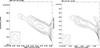 |
Fig. 4. VLA total intensity image of the inner 2-arcsec jet at 6 GHz (left) and 10 GHz (right). The first contour is 0.2 mJy beam−1 at both frequencies. Contours are drawn at [−1,1,1.4,2,2.8,4,5.6,8,16,32,...] times the first contour. The restoring beam is plotted in the bottom left corner. Vectors superimposed on the total intensity contours show the PA of the electric vector, where 0.25-arcsec length corresponds to 2.5 and 0.85 mJy beam−1 (polarization intensity) at 6 and 10 GHz, respectively. The quasar core is located in the bottom right corner just outside the main frame. |
The low fractional polarization of the core (between 2 and 6 percent, depending on the observing frequency) is typical of the central regions of blazars on arcsecond and milliarcsecond scales (e.g., O’Dea et al. 1988; Laurent-Muehleisen et al. 1993; Lister & Homan 2005; Marscher et al. 2002; Harris et al. 2017; Baghel et al. 2024).
3.2. The kiloparsec-scale radio structure
The kiloparsec-scale radio structure of PKS 1127−145 extends for about 30 arcsec (∼250 kpc projected) and is well resolved into several components. Superposed on the faint extended jet emission, we observe three knots (labeled O, A, and B in Fig. 1) before the jet termination at component C. At about 8 arcsec from the core, the jet slightly bends to a PA of ∼50°, in agreement with what is reported in Siemiginowska et al. (2002). A further bend to a PA of ∼40° is observed, corresponding to the outer part of component B marked by component B3 in Fig. 5. Components O and A, at 7.5 and 12 arcsec from the core, respectively, are detected only in the L band, suggesting a steep spectral index. We note that component A was detected in the VLA data at 4.9 GHz presented in Siemiginowska et al. (2007). As was mentioned above, those data were obtained at a lower frequency with a much longer exposure time, and when the array was in a more compact configuration, and are thus sensitive to emission extending on larger angular scales than those recoverable by our observations. The non-detection of component A suggests that its emission is diffuse on scales larger than ∼5 arcsec (i.e., ∼40 kpc).
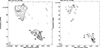 |
Fig. 5. VLA total intensity images of the outer regions of PKS 1127−145 at 6 GHz (left) and 10 GHz (right). The first contour is 0.05 and 0.045 mJy beam−1 at 6 and 10 GHz, respectively, and corresponds to three times the off-source noise level measured far from the core region. Contours are drawn at [−1,1,1.4,2,2.8,4,5.6,8,16,32,...] times the first contour. Vectors superimposed on the total intensity contours show the PA of the electric vector, where 0.5-arcsec length corresponds to 0.1 and 0.08 mJy beam−1 (polarization intensity) at 6 and 10 GHz, respectively. |
Moving farther out, at about 18 arcsec from the core there is component B, detected at all frequencies, which marks a re-brightening of the radio emission, while X-rays fade away. Component B has a fractional polarization of about 20%, similar to the polarization percentage usually found in jet knots (e.g., Bridle et al. 1994). The EVPA is ∼40° at the position of components B1 and B4, roughly parallel to the jet axis at the peak, while it is perpendicular to the total intensity contours at the edges of the component (regions B2, B3, and B5). The EVPA parallel to the jet axis is the opposite of what is found in the inner 2-arcsecond jet region, pinpointing a 90-degree tilt of the magnetic field.
In the 1.5-GHz image, component B is connected to component C by diffuse emission, showing a limb-brightened structure, as is suggested by the brightness profile obtained by interpolating a slice roughly perpendicular to the jet axis with the AIPS task SLICE (Fig. 6).
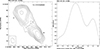 |
Fig. 6. VLA total intensity image at 1.5 GHz (left) of the outer region of PKS 1127−145. The black line indicates the position of the slice used to derive the brightness profile (right). |
The polarized regions B4-B5 and B3 might mark the starting point of the two filaments. Despite being well imaged at 1.5 GHz, at 6 GHz component C is resolved into several polarized clumps with different EVPAs, enshrouded by diffuse emission. On the other hand, at 10 GHz we could detect only subcomponents C2 and C3 and a hint of C1, while the diffuse emission could barely be imaged, likely due to a combination of sensitivity and the largest recoverable angular scale (Fig. 5).
3.3. The kiloparsec-scale X-ray jet
The X-ray jet is well aligned with the 30″ radio jet, showing strong X-ray emitting knots, O and A, leading to more prominent radio knots, B and C. The X-ray knots A and B are connected by the continuous faint X-ray emission. Although faint X-ray emission from knot C is clearly present, no diffuse emission connecting knots B and C is detected (see Fig. 3). Overall, the X-ray surface brightness declines with the distance from the core.
We extracted X-ray spectra of the knots for each observation and fit them separately and then simultaneously by applying an absorbed power law with a Galactic absorption column of NH = 4.09 × 1020 cm−2. The best-fit photon index and an unabsorbed 0.5–7 keV flux resulting from the fit to each knot are presented in Table 4. The results of the simultaneous fitting are consistent between each observations. No significant flux increase is detected in the new Chandra observations. The observed knots’ fluxes are consistent between each observations and within the uncertainties listed in Table 4. The available data are not sensitive to small flux variations at the level of 10−14 erg cm−2 s−1, but we can exclude a flux increase by a factor of 100 in the knots that would dominate over the flux of the core.
X-ray properties of jet knots.
Figure 7 shows the ACIS-S sub-pixel image of knot B. Most of the X-ray counts coincide with the bright and collimated radio part of the knot, but decrease significantly within the fainter fan-like radio emission as the radio jet becomes broader when the X-rays rapidly decline. A shift between the X-ray and radio emission sites could be observed and the X-rays seem to precede the radio emission, as was already claimed in Siemiginowska et al. (2002) by comparing X-rays and 1.4-GHz radio data. Although a misalignment between X-rays and radio emissions seems to be present, the current image does not provide statistically significant measurements of a possible shift. An offset of ∼0.5 arcsec was also claimed by Reddy et al. (2023), who made use of the low-count image reconstruction algorithm. However, the radio data used by Reddy et al. (2023) to investigate the offset have a lower resolution than ours, and the radio peaks may not coincide when different angular resolution are considered, owing to the resolved structure of the component. The same reasoning applies when assessing the offset of component C. The X-ray emission of knot C shown in Fig. 8 is spread uniformly across the diffuse radio structure. The linear polarization map (at 6 GHz) shows a few clumps of enhanced polarization, which seem to be roughly coincident with the stronger X-ray emission. However, the X-ray S/N is very low for any detailed analysis of the knot B and C regions.
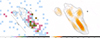 |
Fig. 7. Images of knot B. Left: ACIS-S 0.5–7 keV mosaic image of knot B binned to 0.249″ pixels. The color map shows the number of counts per image pixel. The contours are 6 GHz VLA data starting at 0.075 mJy beam−1 with a |

 |
Fig. 8. Images of knot C. Left: ACIS-S 0.5–7 keV mosaic image of knot C binned to 0.246″ pixels and 6 GHz contours starting at 0.075 mJy beam−1 with a |


3.4. Quasar core in X-rays
We extracted the quasar core spectrum from the circular source region (r = 2″, corresponding to 95% PSF) centered on RA = 11:30:07.11, Dec=−14:49:27.1 in the most recent Chandra observation (ObsId 24911). We fit an absorbed power law model to the spectrum, assuming the Galactic absorption of  , and obtained the best-fit photon index of Γ = 1.28 ± 0.05 and an unabsorbed 0.5–7 keV flux of
  ergs s−1 cm−2. The corresponding 2–10 keV flux for the best fit model is (6.24 ± 0.57)×10−12 ergs s−1 cm−2.
4. Discussion
4.1. The emission mechanism
Although the IC-CMB process often explains the X-ray emission in kiloparsec-scale jets at low and high redshift (e.g., Tavecchio et al. 2000; Sambruna et al. 2004; Erlund et al. 2006; Cheung et al. 2012; Simionescu et al. 2016; Schwartz et al. 2020; Migliori et al. 2022), there are some cases where it clearly fails to reproduce the multiband observations and different scenarios have been proposed (see e.g., Hardcastle 2006; Clautice et al. 2016; Marshall et al. 2018; Tavecchio 2021; Meyer et al. 2023; Reddy et al. 2023).
Past studies of radio and X-ray emission from the extended jet of PKS 1127−145 could not unambiguously unveil the dominant mechanism at the origin of its high-energy emission (Siemiginowska et al. 2007). The X-ray brightness distribution and the offset between the emission peaks in the two bands challenge the standard one-zone leptonic models. The radio and X-ray spectra pointed to more complex jet radiation processes associated with, for example, a “jet-sheath” structure, or multiple epochs of quasar jet activity (Siemiginowska et al. 2007). However, the study was limited by the need to average over unknown jet substructures that could not be resolved by earlier radio observations.
Our full-polarization radio data allow us to investigate for the first time with high angular resolution both the total intensity and polarized emission along the kiloparsec-scale jet. A decrease in X-ray emission with distance from the core, accompanied by an increase in radio emission, though not common, has been observed in other kiloparsec-scale X-ray jets, like 3C 273 (Marshall et al. 2001), 1136−135 and PKS 1510−089 (Sambruna et al. 2004), and 0827+243 (Jorstad & Marscher 2004). In 0827+243 (OJ 248), the X-ray emission shows an apparent bend of ∼90° at about 5 arcsec from the core, and then fades away. On the other hand, at 5 and 15 GHz, the large-scale jet is detected only from the bend up to the jet termination. The bend may correspond to a standing shock wave caused by, for example, a jet-cloud interaction that originates a deflection and a deceleration of the jet flow (Jorstad & Marscher 2004). A similar scenario may apply to PKS 1127−145, where component B may represent a standing shock, after which the jet decelerates. The widening of the jet and its possible limb-brightened structure observed beyond component B support a change in the collimation and velocity of the jet, which may explain the different behavior of the radio and X-ray emission (Georganopoulos & Kazanas 2004). The limb-brightened structure might indicate the coexistence of both longitudinal and transverse velocity gradients at the jet bend.
Although the mean EVPA in quasar jets is usually perpendicular to the jet direction up to the jet termination, where it becomes parallel, it may also change along the jet in the presence of shocks (see e.g., Bridle & Perley 1984; Bridle et al. 1994; Marscher et al. 2002; Pushkarev et al. 2023). This is what is clearly observed in component B of PKS 1127−145, where the magnetic field becomes perpendicular to the jet axis. A change in the EVPA orientation, from perpendicular to parallel to the jet axis, is also observed along the jet of PKS 1510−089, corresponding to a jet bending (O’Dea et al. 1988). The abrupt rotation of the EVPA may be due to the compression of a tangled magnetic field to a plane perpendicular to the jet axis by a shock (Laing 1980). In 0827+243, polarized emission is detected only at the jet termination, precluding the information on the EVPA along the kiloparsec-scale jet. Neither a significant change in the EVPA nor clear bending is observed in the kiloparsec-scale jet of 3C 273 at the position of X-rays dimming (Perley & Meisenheimer 2017). It is worth mentioning that jet bends are not uncommon in the outer regions of relativistic jets (e.g., Bridle et al. 1994) and they are also detected in some kiloparsec-scale jets, showing the same morphology in radio and in X-ray emissions (e.g. 0723+679 and 1150+497, Sambruna et al. 2004), though polarization information is in general unavailable.
A different situation may be represented by component C, where X-ray emission is faint and diluted over a large region. The high angular resolution of our radio data points out a similar situation in the radio band, where the emission is mainly diffuse over several tens of kiloparsecs, while only a marginal part comes from (polarized) compact clumps. Our measurements of the radio polarization in the two outer knots are extremely interesting as they highlight strong organized magnetic fields and potential sites of particle acceleration at hundred-kiloparsec distances from the core. This may signify a possibility for the synchrotron X-rays in large-scale jets, as it is also suggested for hotspots of radio galaxies (e.g., Hardcastle et al. 2004; Orienti et al. 2020a; Migliori et al. 2020). Multifrequency full-polarization observations of a sample of kiloparsec-scale X-ray jets are necessary to draw a more complete view of the physics in these extreme jets.
4.2. The X-ray flaring region
Locating the high-energy flaring region in blazars is not trivial. In the shock-in-jet scenario, a disturbance may be produced at the jet base, and outbursts may take place at different location, as the disturbance propagates down the jet and encounters (quasi-)stationary features. The manifestation of such moving shocks are superluminal jet knots observed on a parsec scale by VLBI observations (see e.g., Marscher et al. 2010; Agudo et al. 2011; Casadio et al. 2015; Jorstad et al. 2017; Lister et al. 2018; Orienti et al. 2020b; Lico et al. 2022; Kramarenko et al. 2022; Weaver et al. 2022). The discovery in the nearby radio galaxy M87 of a high-energy flare taking place in the jet component HST-1 clearly proves that outbursts as bright as the core itself can take place hundred of parsecs away from the central engine (Cheung et al. 2007; Harris et al. 2009). An X-ray flux increase was observed in the jet of Pictor A about 35 kpc from the core (Marshall et al. 2010; Hardcastle et al. 2016). However, in this case the enhancement did not achieve the luminosity of the core of Pictor A.
Neither in X-rays nor at radio frequencies did we observe any brightening of a jet knot in PKS 1127−145. Despite being short, Chandra observations would have been deep enough to detect the flare if it had been from the kiloparsec-scale X-ray jet. On the other hand, the X-ray flux of the quasar core is roughly 2.6 times higher than that reported in Siemiginowska et al. (2002) and comparable to that observed by Swift just after the flaring episode (D’Ammando 2020b), locating the flaring region within the VLA core. We notice that at the redshift of PKS 1127−145 the X-ray flaring component observed in the jet of Pictor A would be about 4 arcsecs from the core (i.e., closer than component O), while M87 HST-1 would be 12 milliarcsec from the core, in the innermost parsec-scale structure. Multi-epoch very long baseline array observations of the central parsec-scale jet region will be presented in a dedicated paper focusing on the multiband analysis of the source core.
5. Conclusions
We have presented results of Chandra X-ray observations and subarcsecond polarimetric VLA observations of PKS 1127−145 performed during a flaring event detected in γ-rays by Fermi-LAT. The conclusions we can draw from this study are:
-
The high angular resolution of the new VLA data allowed us to image the kiloparsec-scale inner jet for the first time. The inner jet is highly polarized and the magnetic field is parallel to the jet axis.
-
In agreement with earlier observations, the outer knots are brighter in radio, contrary to what is found in X-rays. A re-brightening of the radio emission is observed at about 150 kpc (projected) from the core, where the jet slightly bends and likely decelerates. The magnetic field at the position of the bend shows a 90-degree rotation, likely due to compression to a plane perpendicular to the jet axis, as is observed in many knots of relativistic jets, though usually on a parsec scale.
-
The outermost component is resolved into several polarized compact regions enshrouded by diffuse emission. Such a patchy structure, reminiscent of some hotspots in radio galaxies, should be kept in consideration when modeling the spectral energy distribution of these kiloparsec-scale structures.
-
The limb-brightened structure and the widening of the jet connecting component B to the jet termination support a deceleration and decollimation of the jet flow in the outer part of PKS 1127−145.
-
The X-ray flux from the quasar core is consistent with the Swift measurements during the 2020–2021 flaring period; that is, 2.6 times higher than the flux in the 2000 data reported by Siemiginowska et al. (2002). Neither radio nor strong X-ray flux variability is observed from any region of the kiloparsec-scale jet at the level detected by Swift. This strongly indicates that the high-energy flaring episode was located in the VLA core.
The faint X-ray emission from the outermost knots prevents a detailed study of the correlation between radio and X-ray emission at the edge of the jet. Deep X-ray observations are necessary, then, to investigate whether the X-ray morphology is consistent with the radio structure, with clumps and filaments, and to determine any alignment and/or separation of individual features in the bands. Recently, the high angular resolution of LOw-Frequency ARray observations in the MHz regime pointed out that the flux density at 150 MHz of the knots in the jet of 4C +19.44 are below the values expected by extrapolating the GHz spectra, suggesting a low-energy curvature of the particle energy distribution (Harris et al. 2019). The jump in resolution and sensitivity in the MHz regime that will be achieved with the advent of the Square Kilometre Array, together with multiband information, will provide important information on the electron energy distribution, particle acceleration, and energy dissipation at the periphery of relativistic jets. However, the required high-angular-resolution X-ray imaging is currently only achievable in the Chandra observations and a comparable, or better, resolution will not be possible until a new generation of telescopes, such as the planned Lynx (Gaskin et al. 2019) mission, are built.
For information on the Chandra data see: https://cxc.harvard.edu/proposer/POG/html/index.html
The parsec-scale jet structure imaged by the Very Long Baseline Array at milliarcsecond-scale resolution will be presented in a forthcoming paper.
Acknowledgments
We thank the anonymous referee for reading the manuscript carefully and making valuable suggestions. We wish to thank Patrick Slane, Director of the Chandra X-ray Center, for approving our DDT request, and the Chandra team for carrying out the new observations (obsid 24911). The VLA is operated by the US National Radio Astronomy Observatory which is a facility of the National Science Foundation operated under cooperative agreement by Associated Universities, Inc. This work has made use of the NASA/IPAC Extragalactic Database (NED) which is operated by the JPL, California Institute of Technology, under contract with the National Aeronautics and Space Administration. This research has made use of data obtained from the Chandra Data Archive and software provided by the Chandra X-ray Center (CXC) in the application packages CIAO and Sherpa. A.S. was supported by NASA contract NAS8-03060 (Chandra X-ray Center).
References
- Abdo, A. A., Ackermann, M., Agudo, I., et al. 2011, ApJ, 733, L26 [NASA ADS] [CrossRef] [Google Scholar]
- Abdollahi, S., Acero, F., Ackermann, M., et al. 2020, ApJS, 247, 33 [Google Scholar]
- Acharyya, A., Chadwick, P. M., & Brown, A. M. 2021, MNRAS, 500, 5297 [Google Scholar]
- Ackermann, M., Anantua, R., Asano, K., et al. 2016, ApJ, 824, L20 [NASA ADS] [CrossRef] [Google Scholar]
- Agudo, I., Jorstad, S. G., Marscher, A. P., et al. 2011, ApJ, 726, L13 [NASA ADS] [CrossRef] [Google Scholar]
- Angioni, R. 2020, ATel., 14260 [Google Scholar]
- Baghel, J., Kharb, P., Hovatta, T., et al. 2024, MNRAS, 527, 672 [Google Scholar]
- Bridle, A. H., & Perley, R. A. 1984, ARA&A, 22, 319 [NASA ADS] [CrossRef] [Google Scholar]
- Bridle, A. H., Hough, D. H., Lonsdale, C. J., Burns, J. O., & Laing, R. A. 1994, AJ, 108, 766 [NASA ADS] [CrossRef] [Google Scholar]
- Casadio, C., Gómez, J. L., Jorstad, S. G., et al. 2015, ApJ, 813, 51 [Google Scholar]
- Cheung, C. C., Harris, D. E., & Stawarz, L. 2007, ApJ, 663, L65 [NASA ADS] [CrossRef] [Google Scholar]
- Cheung, C. C., Stawarz, L., Siemiginowska, A., et al. 2012, ApJ, 756, L20 [NASA ADS] [CrossRef] [Google Scholar]
- Clautice, D., Perlman, E. S., Georganopoulos, M., et al. 2016, ApJ, 826, 109 [NASA ADS] [CrossRef] [Google Scholar]
- Cornwell, T., & Fomalont, E. B. 1999, ASPC, 180, 187 [NASA ADS] [Google Scholar]
- Costamante, L., Cutini, S., Tosti, G., Antolini, E., & Tramacere, A. 2018, MNRAS, 477, 4749 [Google Scholar]
- D’Ammando, F. 2020a, ATel., 14265 [Google Scholar]
- D’Ammando, F. 2020b, ATel., 14280 [Google Scholar]
- D’Ammando, F., Raiteri, C. M., Villata, M., et al. 2019, MNRAS, 490, 5300 [Google Scholar]
- Drinkwater, M. J., Webster, R. L., Francis, P. J., et al. 1997, MNRAS, 284, 85 [NASA ADS] [Google Scholar]
- Erlund, M. C., Fabian, A. C., Blundell, K. M., Celotti, A., & Crawford, C. S. 2006, MNRAS, 371, 29 [Google Scholar]
- Freeman, P., Doe, S., & Siemiginowska, A. 2001, Proc. SPIE, 4477, 76 [Google Scholar]
- Fruscione, A., McDowell, J. C., Allen, G. E., et al. 2006, Proc. SPIE, 6270, 1 [Google Scholar]
- Gaskin, J. A., Swartz, D. A., Vikhlinin, A., et al. 2019, JATIS, 5, 021001 [NASA ADS] [Google Scholar]
- Georganopoulos, M., & Kazanas, D. 2004, ApJ, 604, L81 [NASA ADS] [CrossRef] [Google Scholar]
- Hada, K., Giroletti, M., Kino, M., et al. 2014, ApJ, 788, 165 [NASA ADS] [CrossRef] [Google Scholar]
- Hardcastle, M. J. 2006, MNRAS, 366, 1465 [Google Scholar]
- Hardcastle, M. J., Harris, D. E., Worrall, D. M., & Birkinshaw, M. 2004, ApJ, 612, 729 [Google Scholar]
- Hardcastle, M. J., Croston, J. H., & Kraft, R. P. 2007, ApJ, 669, 893 [NASA ADS] [CrossRef] [Google Scholar]
- Hardcastle, M. J., Lenc, E., Birkinshaw, M., et al. 2016, MNRAS, 455, 3526 [NASA ADS] [CrossRef] [Google Scholar]
- Harris, D. E., Cheung, C. C., Stawarz, Ł., et al. 2009, ApJ, 699, 305 [NASA ADS] [CrossRef] [Google Scholar]
- Harris, D. E., Lee, N. P., Schwartz, D. A., et al. 2017, ApJ, 846, 119 [NASA ADS] [CrossRef] [Google Scholar]
- Harris, D. E., Moldón, J., Oonj, J. R. R., et al. 2019, ApJ, 873, 21 [NASA ADS] [CrossRef] [Google Scholar]
- Hayashida, M., Nalevajko, K., Madejski, G. M., et al. 2015, ApJ, 807, 79 [NASA ADS] [CrossRef] [Google Scholar]
- Homan, D. C., Wardle, J. F. C., Cheung, C. C., Roberts, D. H., & Attridge, J. M. 2002, ApJ, 580, 742 [Google Scholar]
- Ighina, L., Moretti, A., Tavecchio, F., et al. 2022, A&A, 659, 93 [Google Scholar]
- Jorstad, S. G., & Marscher, A. P. 2004, ApJ, 614, 615 [NASA ADS] [CrossRef] [Google Scholar]
- Jorstad, S., Marscher, A. P., Morozova, D. A., et al. 2017, ApJ, 846, 98 [NASA ADS] [CrossRef] [Google Scholar]
- Kramarenko, I. G., Pushkarev, A. B., Kovalev, Y. Y., et al. 2022, MNRAS, 510, 469 [Google Scholar]
- Laing, R. A. 1980, MNRAS, 193, 439 [NASA ADS] [Google Scholar]
- Laurent-Muehleisen, S. A., Kollgaard, R. I., Moellenbrock, G. A., & Feigelson, E. D. 1993, AJ, 106, 875 [NASA ADS] [CrossRef] [Google Scholar]
- Lico, R., Casadio, C., Jorstad, S. G., et al. 2022, A&A, 658, 10 [Google Scholar]
- Lister, M., & Homan, D. C. 2005, AJ, 130, 1389 [NASA ADS] [CrossRef] [Google Scholar]
- Lister, M. L., Aller, M. F., Aller, H. D., et al. 2018, ApJS, 234, 12 [CrossRef] [Google Scholar]
- Marscher, A. P., Jorstad, S. G., Mattox, J. R., & Wehrle, A. E. 2002, ApJ, 577, 85 [NASA ADS] [CrossRef] [Google Scholar]
- Marscher, A. P., Jorstad, S. G., D’Arcangelo, F. D., et al. 2008, Nature, 452, 966 [Google Scholar]
- Marscher, A. P., Jorstad, S. G., Larionov, V. M., et al. 2010, ApJ, 710, L126 [Google Scholar]
- Marshall, H. L., Harris, D. E., Grimes, J. P., et al. 2001, ApJ, 549, L167 [NASA ADS] [CrossRef] [Google Scholar]
- Marshall, H. L., Hardcastle, M. J., Birkinshaw, M., et al. 2010, ApJ, 714, L213 [NASA ADS] [CrossRef] [Google Scholar]
- Marshall, H. L., Gelbord, J. M., Worrall, D. M., et al. 2018, ApJ, 856, 66 [NASA ADS] [CrossRef] [Google Scholar]
- McKeough, K., Siemiginowska, A., Cheung, C. C., et al. 2016, ApJ, 833, 123 [NASA ADS] [CrossRef] [Google Scholar]
- McMullin, J. P., Waters, B., Schiebel, D., Young, W., & Golap, K. 2007, ASP Conf. Ser., 376, 127 [Google Scholar]
- Meyer, E. T., Shaik, A., Tang, Y., et al. 2023, Nat. Astron., 7, 967 [NASA ADS] [CrossRef] [Google Scholar]
- Migliori, G., Orienti, M., Coccato, L., et al. 2020, MNRAS, 495, 1593 [NASA ADS] [CrossRef] [Google Scholar]
- Migliori, G., Siemiginowska, A., Cheung, C. C., et al. 2022, MNRAS, 512, 4639 [NASA ADS] [CrossRef] [Google Scholar]
- Mingo, B., Hardcastle, M. J., Ineson, J., et al. 2017, MNRAS, 470, 2762 [Google Scholar]
- O’Dea, C. P., Barvainis, R., & Challis, P. M. 1988, AJ, 96, 435 [CrossRef] [Google Scholar]
- Orienti, M., Venturi, T., Dallacasa, D., et al. 2011, MNRAS, 417, 359 [NASA ADS] [CrossRef] [Google Scholar]
- Orienti, M., Koyama, S., D’Ammando, F., et al. 2013, MNRAS, 428, 2418 [Google Scholar]
- Orienti, M., Migliori, G., Brunetti, G., et al. 2020a, MNRAS, 494, 2244 [NASA ADS] [CrossRef] [Google Scholar]
- Orienti, M., D’Ammando, F., Giroletti, M., et al. 2020b, MNRAS, 491, 858 [NASA ADS] [CrossRef] [Google Scholar]
- Perley, R. A., & Butler, B. J. 2017, ApJS, 230, 7 [NASA ADS] [CrossRef] [Google Scholar]
- Perley, R. A., & Meisenheimer, K. 2017, A&A, 601, 35 [Google Scholar]
- Pushkarev, A. B., Aller, H. D., Aller, M. F., et al. 2023, MNRAS, 520, 6053 [NASA ADS] [CrossRef] [Google Scholar]
- Reddy, K., Georganopoulos, M., Meyer, E. T., Keenan, M., & Kollmann, K. E. 2023, ApJS, 265, 8 [NASA ADS] [CrossRef] [Google Scholar]
- Refsdal, R., Doe, S., Nguyen, D., et al. 2011, ASPC, 442, 687 [NASA ADS] [Google Scholar]
- Sambruna, R. M., Gambill, J. K., Maraschi, L., et al. 2004, ApJ, 608, 698 [Google Scholar]
- Schwartz, D. A., Siemiginowska, A., Snios, B., et al. 2020, ApJ, 904, 57 [NASA ADS] [CrossRef] [Google Scholar]
- Siemiginowska, A., Bechtold, J., Aldcroft, T. L., et al. 2002, ApJ, 570, 543 [NASA ADS] [CrossRef] [Google Scholar]
- Siemiginowska, A., Stawarz, L., Cheung, C. C., et al. 2007, ApJ, 657, 145 [NASA ADS] [CrossRef] [Google Scholar]
- Simionescu, A., Stawarz, L., Ichinohe, Y., et al. 2016, ApJ, 816, L15 [NASA ADS] [CrossRef] [Google Scholar]
- Tavecchio, F., Marasca, L., Sambruna, R. M., & Urry, C. M. 2000, ApJ, 544, L23 [NASA ADS] [CrossRef] [Google Scholar]
- Tavecchio, F. 2021, MNRAS, 501, 6199 [Google Scholar]
- Tingay, S. J., Lenc, E., Brunetti, G., & Bondi, M. 2008, ApJ, 136, 2473 [CrossRef] [Google Scholar]
- Weaver, Z. R., Jorstad, S. G., Marscher, A. M., et al. 2022, ApJS, 260, 12 [NASA ADS] [CrossRef] [Google Scholar]
- Wright, E. L. 2006, PASP, 118, 1711 [NASA ADS] [CrossRef] [Google Scholar]
All Tables
All Figures
|
Fig. 1. Total intensity images of PKS 1127−145 at 1.5 GHz (top), 6 GHz (middle), and 10 GHz (bottom). The first contour is 0.6, 0.1, and 0.075 mJy beam−1 at 1.5, 6, and 10 GHz, respectively, and corresponds to three times the rms measured on the image plane close to the center. Contours are drawn at [−1, 1, 1.4, 2, 2.8, 4, 5.6, 8, 16, 32, 64,...] times the first contour. The restoring beam is plotted in the bottom left corner of each image. |
| In the text | |
|
Fig. 2. ACIS-S 0.5-7 keV image showing the total number of counts per pixel obtained in each Chandra observation. The Chandra ObsID number is indicated in the bottom right corner of each panel, from left to right: 866, 5708, and 24911. The image pixels are the native ACIS-S pixel size of 0.492″. The image is displayed on a logarithmic scale with the color bar scale indicating the number of counts per pixel. In addition to the jet, the readout streak (labeled green) is visible with different angles dependent on the Chandra roll angle during the observation. |
| In the text | |
|
Fig. 3. ACIS-S 0.5–7 keV mosaic image binned into 0.246″ pixels (0.5 bin scale). The color bar shows the number of counts per pixel. The black contours are from the 1.6 GHz L-band VLA map starting at 0.45 mJy beam−1 and increasing by |
| In the text | |
|
Fig. 4. VLA total intensity image of the inner 2-arcsec jet at 6 GHz (left) and 10 GHz (right). The first contour is 0.2 mJy beam−1 at both frequencies. Contours are drawn at [−1,1,1.4,2,2.8,4,5.6,8,16,32,...] times the first contour. The restoring beam is plotted in the bottom left corner. Vectors superimposed on the total intensity contours show the PA of the electric vector, where 0.25-arcsec length corresponds to 2.5 and 0.85 mJy beam−1 (polarization intensity) at 6 and 10 GHz, respectively. The quasar core is located in the bottom right corner just outside the main frame. |
| In the text | |
|
Fig. 5. VLA total intensity images of the outer regions of PKS 1127−145 at 6 GHz (left) and 10 GHz (right). The first contour is 0.05 and 0.045 mJy beam−1 at 6 and 10 GHz, respectively, and corresponds to three times the off-source noise level measured far from the core region. Contours are drawn at [−1,1,1.4,2,2.8,4,5.6,8,16,32,...] times the first contour. Vectors superimposed on the total intensity contours show the PA of the electric vector, where 0.5-arcsec length corresponds to 0.1 and 0.08 mJy beam−1 (polarization intensity) at 6 and 10 GHz, respectively. |
| In the text | |
|
Fig. 6. VLA total intensity image at 1.5 GHz (left) of the outer region of PKS 1127−145. The black line indicates the position of the slice used to derive the brightness profile (right). |
| In the text | |
|
Fig. 7. Images of knot B. Left: ACIS-S 0.5–7 keV mosaic image of knot B binned to 0.249″ pixels. The color map shows the number of counts per image pixel. The contours are 6 GHz VLA data starting at 0.075 mJy beam−1 with a |
| In the text | |
|
Fig. 8. Images of knot C. Left: ACIS-S 0.5–7 keV mosaic image of knot C binned to 0.246″ pixels and 6 GHz contours starting at 0.075 mJy beam−1 with a |
| In the text | |
Current usage metrics show cumulative count of Article Views (full-text article views including HTML views, PDF and ePub downloads, according to the available data) and Abstracts Views on Vision4Press platform.
Data correspond to usage on the plateform after 2015. The current usage metrics is available 48-96 hours after online publication and is updated daily on week days.
Initial download of the metrics may take a while.