| Issue |
A&A
Volume 687, July 2024
|
|
|---|---|---|
| Article Number | A265 | |
| Number of page(s) | 26 | |
| Section | Stellar structure and evolution | |
| DOI | https://doi.org/10.1051/0004-6361/202348369 | |
| Published online | 30 July 2024 | |
Non-linear three-mode coupling of gravity modes in rotating slowly pulsating B stars
Stationary solutions and modeling potential
1
Institute of Astronomy, KU Leuven, Celestijnenlaan 200D, 3001 Leuven, Belgium
e-mail: This email address is being protected from spambots. You need JavaScript enabled to view it.
2
TAPIR, Mailcode 350-17, California Institute of Technology, Pasadena, CA 91125, USA
3
Kavli Institute for Theoretical Physics, University of California, Santa Barbara, CA 93106, USA
4
Royal Observatory of Belgium, Ringlaan 3, Brussels, Belgium
5
Dept. of Astrophysics, IMAPP, Radboud University Nijmegen, 6500 GL Nijmegen, The Netherlands
6
Max Planck Institute for Astronomy, Koenigstuhl 17, 69117 Heidelberg, Germany
7
Guest Researcher, Center for Computational Astrophysics, Flatiron Institute, 162 Fifth Ave, New York, NY 10010, USA
Received:
23
October
2023
Accepted:
21
December
2023
Abstract
Context. Slowly pulsating B (SPB) stars display multi-periodic variability in the gravito-inertial mode regime with indications of non-linear resonances between modes. Several have undergone asteroseismic modeling in the past few years to infer their internal properties, but only in a linear setting. These stars rotate fast, so that rotation is typically included in the modeling by means of the traditional approximation of rotation (TAR).
Aims. We aim to extend the set of tools available for asteroseismology, by describing time-independent (stationary) resonant non-linear coupling among three gravito-inertial modes within the TAR. Such coupling offers the opportunity to use mode amplitude ratios in the asteroseismic modeling process, instead of only relying on frequencies of linear eigenmodes, as has been done so far.
Methods. Following observational detections, we derive expressions for the resonant stationary non-linear coupling between three gravito-inertial modes in rotating stars. We assess selection rules and stability domains for stationary solutions. We also predict non-linear frequencies and amplitude ratio observables that can be compared with their observed counterparts.
Results. The non-linear frequency shifts of stationary couplings are negligible compared to typical frequency errors derived from observations. The theoretically predicted amplitude ratios of combination frequencies match with some of their observational counterparts in the SPB targets. Other, unexplained observed ratios could be linked to other saturation mechanisms, to interactions between different modes, or to different opacity gradients in the driving zone.
Conclusions. For the purpose of asteroseismic modeling, our non-linear mode coupling formalism can explain some of the stationary amplitude ratios of observed resonant mode couplings in single SPB stars monitored during 4 years by the Kepler space telescope.
Key words: asteroseismology / stars: evolution / stars: interiors / stars: oscillations / stars: rotation / stars: variables: general
© The Authors 2024
 Open Access article, published by EDP Sciences, under the terms of the Creative Commons Attribution License (https://creativecommons.org/licenses/by/4.0), which permits unrestricted use, distribution, and reproduction in any medium, provided the original work is properly cited.
This article is published in open access under the Subscribe to Open model. This email address is being protected from spambots. You need JavaScript enabled to view it. to support open access publication.
1. Introduction
Slowly pulsating B (SPB) stars are mid-to-late-B variable stars on the main sequence that display a variety of low-frequency oscillations, and have masses ranging from ∼3 to ∼9 M⊙ (e.g., Waelkens 1991; De Cat & Aerts 2002; Pedersen et al. 2021; Szewczuk et al. 2021). Much of their multi-periodic variability is attributed to gravity modes excited by the κ mechanism associated with the Fe opacity bump in their envelope (Gautschy & Saio 1993; Dziembowski et al. 1993; Pamyatnykh 1999). Their rotation rates vary from ∼1% of critical to nearly critical velocity. The Coriolis force is a significant restoring force for most SPB oscillations, in addition to buoyancy (e.g., Lee 2012; Pedersen et al. 2021). We refer to such gravito-inertial modes whenever we mention g modes in this work. The large number of oscillations identified in space photometry of SPB stars have made them the subject of many asteroseismic modeling studies in the past few years (e.g., Degroote et al. 2010; Szewczuk & Daszyńska-Daszkiewicz 2018; Walczak et al. 2019; Wu & Li 2019; Wu et al. 2020; Szewczuk et al. 2021; Pedersen et al. 2021; Szewczuk et al. 2022).
The broad general review of asteroseismology by Aerts (2021, and references therein) makes it clear that stellar modeling is currently mainly done in a linear framework. Signals with frequencies approximately equal to linear combinations of frequencies of other detected signals, termed combination frequencies, are often detected in frequency lists generated by the harmonic analyses of stellar variability commonly used in asteroseismology (Aerts et al. 2010). Some of these combination frequencies can be explained by a non-linear response of the stellar medium to the pulsation wave (see e.g., Bowman et al. 2016), which is referred to as non-linear distortion by Degroote et al. (2009). In this work, however, we focus on combination frequencies that are explained by non-linear coupling among oscillation modes (e.g., Buchler & Goupil 1984 and Van Hoolst 1994b). The amplitudes of heat-driven non-radial oscillations in SPB stars cannot be explained in the linear approximation. Observed amplitudes are therefore currently not used in asteroseismic inference. Non-linear mode interactions that exchange energy among (coupled) modes must be taken into account to describe g mode amplitude limitation. Such interactions also change the mode frequencies. Instead of resorting to resource-costly numerical integration of the non-linear hydrodynamical equations that govern the oscillation dynamics, we consider weakly non-linear effects of the lowest order. We therefore consider isolated weak non-linear mode coupling among three g modes, and followed and extended the approach of Lee (2012), hereafter referred to as L12. Our approach is guided by the detected properties of SPB stars in Kepler observations, which are summarized in the sample studies by Pedersen et al. (2021) and Szewczuk et al. (2021).
Weak non-linear mode coupling among three modes has been a topic of interest for stellar pulsation modes since the 1970s, with several seminal papers written long before space photometry was available (limiting ourselves to mode coupling among non-radial pulsations, see e.g., Dziembowski 1982, 1993; Buchler & Regev 1983; Aikawa 1984; Moskalik 1985; Dziembowski & Krolikowska 1985; Dappen & Perdang 1985; Dziembowski et al. 1988; Van Hoolst & Smeyers 1993; Buchler 1993; Takeuti & Buchler 1993; Van Hoolst 1994a,b, 1995; Van Hoolst 1996; Goupil & Buchler 1994; Buchler et al. 1995, 1997; Goupil et al. 1998; Wu & Goldreich 2001). Most of these formalisms focused on the description of mode coupling in non-rotating stars. A notable exception is the formalism developed by Friedman and Schutz (Friedman & Schutz 1978a,b; Schutz 1979), on which Schenk et al. (2001), hereafter referred to as S01, based their treatment of non-linear three-mode coupling in rotating stars. S01 included the effects of the Coriolis force perturbatively, but their framework is generic, allowing for the derivation of formalisms that do not treat the Coriolis force as a perturbation. Several studies are based on the S01 formalism, modeling non-linear tides in multiple-star systems (e.g., Fuller & Lai 2012; Burkart et al. 2012, 2013, 2014; Fuller et al. 2013; O’Leary & Burkart 2014; Weinberg 2016; Fuller 2017; Guo 2020; Yu et al. 2020, 2021a; Zanazzi & Wu 2021) and in star-exoplanet systems (Essick & Weinberg 2016; Vick et al. 2019; Yu et al. 2021b, 2022), non-linear interactions among modes in neutron stars (e.g., Morsink 2002; Arras et al. 2003; Lai & Wu 2006; Weinberg & Quataert 2008; Weinberg et al. 2013), tidal migration in the moon systems of Jupiter and Saturn (Fuller et al. 2016), non-linear interactions among mixed modes in red giant stars (Weinberg & Arras 2019; Weinberg et al. 2021), or resonant mode coupling in δ Sct stars (Mourabit & Weinberg 2023).
L12 used the S01 formalism as a basis for an extension that described rapidly rotating stars in which the Coriolis force cannot be treated as a perturbation. To do so, they adopted the so-called traditional approximation for rotation (TAR), in which the latitudinal component of the rotation vector in a spherical coordinate system was neglected, assuming spherical symmetry. This decoupled the radial and horizontal components of the pulsation equations (e.g., Longuet-Higgins 1968; Lee & Saio 1997; Townsend 2003; Mathis 2013). For high-radial order g modes it is justified to ignore the centrifugal force within the TAR, because the dominant contribution to the mode energy occurs deep inside the star, close to the convective core, where rotational deformation is small and spherical symmetry is a good approximation (Mathis & Prat 2019; Henneco et al. 2021; Dhouib et al. 2021a,b). There is a marked difference in scale of the rotation frequency Ω and the Brunt-Väisälä frequency N in those deep near-core regions. The assumption that the Coriolis force is weaker than the buoyancy force in the direction of stable entropy or chemical stratification is therefore fulfilled near the core for low-frequency (Poincaré) modes1. Their horizontal velocities are also greater than the vertical velocities (see Mathis & Prat 2019), justifying the neglect of the latitudinal rotation vector component within the TAR.
L12 used their quadratic non-linear mode coupling formalism within the TAR (based on the S01 formalism) to provide a numerical mode coupling example for a specific SPB star model near the zero-age main sequence. The computed mode properties of that example were not compared to observed SPB mode properties. In this work we extend and correct the L12 formalism with the aim of creating a modeling framework that can be used to model non-linear three-mode coupling of g modes in some of the 38 SPB stars considered by Van Beeck et al. (2021), hereafter referred to as V21. We specifically focus on deriving the conditions for which the amplitudes of modes in coupled mode triads, and their combination phase, do not vary over time. The mode parameters inferred by V21 allowed for the discovery of many such potentially ‘locked’ mode couplings. We therefore contrast the theoretically predicted observables computed by our formalism for mode couplings obtained from models typical for the ensemble of SPB stars analyzed by V21 with their detected observational counterparts. We first provide a rigorous overview of our theoretical oscillation model in Sect. 2, followed by Sect. 3, which describes the non-linear theoretical observables. In Sect. 4 we show the numerical results for resonant mode couplings typical for SPB stars, while Sect. 5 discusses the potential of our theoretical framework for future asteroseismic modeling. Finally, Sect. 6 outlines our conclusions and prospects.
2. Theoretical oscillation model
2.1. Linear free oscillations within the TAR
The linearized momentum equation governing linear stellar oscillations in uniformly rotating stars is expressed in a co-rotating reference frame as (e.g., Frieman & Rotenberg 1960, Lynden-Bell & Ostriker 1967 or S01)
 (1)
(1)
where ξ denotes the Lagrangian displacement, the superscripted dot indicates a partial time derivative,  is the Coriolis term, with Ω = Ω ez the (uniform) rotation vector and ez the unit vector along the rotation axis, C(ξ) is the term that describes forces not depending on the oscillation frequency, and aext is any acceleration due to external forces. For the free oscillations used in linear asteroseismology, aext = 0. The operators B and C are anti-Hermitian and Hermitian, respectively (Lynden-Bell & Ostriker 1967). An equivalent tensor representation of the linearized momentum equation is described in Appendix A and used in Sect. 2.3.
With time dependence Ansatz
 (2)
(2)
we can rewrite Eq. (1) for free oscillations as
 (3)
(3)
where ω is the (real- or complex-valued) angular frequency in the co-rotating frame (e.g., Friedman & Schutz 1978a, S01 and Prat et al. 2019). The Hermiticity of the operators iB and C allow one to define a generic orthogonality relation valid for two distinct (ordinary) eigenmodes ξφ and ξβ of Eq. (3) if  and Ω is time-independent, where we use the superscript ‘*’ to indicate a complex conjugated quantity,
 (4)
(4)
In Eq. (4), the inner product of the Hilbert space ℋ spanned by the complex eigenvectors ξ and ξ′ of Eq. (3) is defined as
 (5)
(5)
A proof of the orthogonality condition implied in Eq. (4) for the two distinct modes ξφ and ξβ is given in Appendix B. For a mode φ with complex-valued ωφ described by Eq. (3), the linear heat-driven growth (damping) rate γφ is defined as γφ ≡ Im[ωφ]. Because of Ansatz (2), linear growth (damping) occurs when γφ is positive (negative).
We describe the coupling among non-degenerate modes using their adiabatic eigenfunctions (in Sect. 2.3), for which the generic orthogonality relation implied in Eq. (4) for the modes φ and β can be written as (see Appendix B and S01)
 (6)
(6)
where  denotes a Kronecker delta, Re[ωφ] = Ωφ (and similar for mode β), and the real-valued constant bφ is given by
 (7)
(7)
The constant bφ defined in Eq. (7) is related to the rotating-frame mode energy ϵφ at unit complex amplitude, if Ωφ ≠ 0 (S01):
 (8)
(8)
Because we describe uniformly rotating non-magnetic stars and use the Cowling approximation in which the Eulerian perturbation of the gravitational potential is set to zero,
 (9)
(9)
with δP and δρ being the Eulerian perturbations of the pressure and density around their equilibrium values P and ρ (e.g., P19). The explicit dependence of C(ξ) on ξ is defined in, for example, Lynden-Bell & Ostriker (1967).
We use the TAR, which ignores the latitudinal component − Ω sinθ eθ of the rotation vector (e.g., Lee & Saio 1997). The Lagrangian displacement of a g mode φ can then be expressed in spherical coordinates (r, θ, ϕ) as (Prat et al. 2019)
![Mathematical equation: $$ \begin{aligned} {\boldsymbol{\xi }}_\varphi = [\xi _r^\varphi (r)\,H_r(\theta ),\,\xi _h^\varphi (r)\,H_{\theta }(\theta ),\,i\,\xi _h^\varphi (r)\,H_{\phi }(\theta )]\,e^{i\,(m_\varphi \,\phi _\varphi \,-\,\Omega _\varphi \,t)}\,, \end{aligned} $$](/articles/aa/full_html/2024/07/aa48369-23/aa48369-23-eq13.gif) (10)
(10)
where mφ is the mode azimuthal order, ϕφ is the mode phase,  and
and  are the radial and horizontal mode displacement components, and Hr(θ), Hθ(θ) and Hϕ(θ) are the real-valued radial, latitudinal and azimuthal Hough functions of a mode φ (see Appendix A of Prat et al. 2019 for their definitions). Following L12, we normalize radial Hough function Hr(θ) as
 (11)
(11)
where μ = cosθ. The normalization of Hr(θ) also determines the normalization of the latitudinal and azimuthal Hough functions Hθ(θ) and Hϕ(θ).
2.2. Non-linear oscillations within the TAR
Non-linear mode interactions add acceleration (i.e., forcing) terms to the governing equation of motion, so that the higher-order equation of motion becomes the following quadratic eigenfunction problem (see e.g., Frieman & Rotenberg 1960)
![Mathematical equation: $$ \begin{aligned} -\, \omega ^2 \boldsymbol{\xi } - i\, \omega \, \boldsymbol{B}\left(\boldsymbol{\xi }\right) + \boldsymbol{C}\left(\boldsymbol{\xi }\right) = \boldsymbol{a}[\boldsymbol{\xi }]\,, \end{aligned} $$](/articles/aa/full_html/2024/07/aa48369-23/aa48369-23-eq17.gif) (12)
(12)
under the Ansatz given by Eq. (2): ξ(x, t)=ξ(x) e−iωt. In Eq. (12), the first term describes the acceleration. That acceleration is changed by the non-linear coupling term a[ξ], which can be split up into contributions from pressure gradients (aP[ξ]) and gravity (aG[ξ]).
Because we limit ourselves to non-linear three-mode interactions, it is sufficient to expand a[ξ] to second order (e.g., S01),
![Mathematical equation: $$ \begin{aligned} \boldsymbol{a}[\boldsymbol{\xi }] = \boldsymbol{a}^{(2)}[\boldsymbol{\xi },\boldsymbol{\xi }^\prime ] + O\left(\boldsymbol{\xi }^3\right) = \boldsymbol{a}^{(2)}_P[\boldsymbol{\xi },\boldsymbol{\xi }^\prime ] + \boldsymbol{a}^{(2)}_G[\boldsymbol{\xi },\boldsymbol{\xi }^\prime ] + O\left(\boldsymbol{\xi }^3\right), \end{aligned} $$](/articles/aa/full_html/2024/07/aa48369-23/aa48369-23-eq18.gif) (13)
(13)
where a(2)[ξ, ξ′], the second order pressure term ![Mathematical equation: $ \boldsymbol{a}^{(2)}_P[\boldsymbol{\xi},\boldsymbol{\xi}^\prime] $](/articles/aa/full_html/2024/07/aa48369-23/aa48369-23-eq19.gif) , and the second order gravitational acceleration term
, and the second order gravitational acceleration term ![Mathematical equation: $ \boldsymbol{a}^{(2)}_G[\boldsymbol{\xi},\boldsymbol{\xi}^\prime] $](/articles/aa/full_html/2024/07/aa48369-23/aa48369-23-eq20.gif) are symmetric bilinear functions of the Lagrangian displacements associated with the interacting modes. The nth components of
are symmetric bilinear functions of the Lagrangian displacements associated with the interacting modes. The nth components of ![Mathematical equation: $ \boldsymbol{a}^{(2)}_P[\boldsymbol{\xi},\boldsymbol{\xi}^\prime] $](/articles/aa/full_html/2024/07/aa48369-23/aa48369-23-eq21.gif) and
and ![Mathematical equation: $ \boldsymbol{a}^{(2)}_G[\boldsymbol{\xi},\boldsymbol{\xi}^\prime] $](/articles/aa/full_html/2024/07/aa48369-23/aa48369-23-eq22.gif) are expressed as (e.g., S01)
are expressed as (e.g., S01)
![Mathematical equation: $$ \begin{aligned} \boldsymbol{a}^{(2)}_{G,\,n}[\boldsymbol{\xi },\boldsymbol{\xi }^\prime ] =&\, -\dfrac{1}{2}\,\xi ^k\,\xi ^l\,\nabla _k\,\nabla _l\,\nabla _n\,\Phi \,,\end{aligned} $$](/articles/aa/full_html/2024/07/aa48369-23/aa48369-23-eq23.gif) (14a)
(14a)
![Mathematical equation: $$ \begin{aligned} \boldsymbol{a}^{(2)}_{P,\,n}[\boldsymbol{\xi },\boldsymbol{\xi }^\prime ] =&\, -\dfrac{1}{\rho }\,\nabla _j\left[p\,\left(\Gamma _1 - 1\right)\Theta ^j_n + p\,\Xi ^j_n + \Psi \,\delta _n^j\right]\,, \end{aligned} $$](/articles/aa/full_html/2024/07/aa48369-23/aa48369-23-eq24.gif) (14b)
(14b)
where we use the Cowling approximation and the Einstein summation convention, ∇φ denotes the covariant derivative with respect to coordinate xφ, the adiabatic exponent Γ1 = (∂lnp/∂lnρ)S with subscript S denoting adiabatic conditions, and Φ is the gravitational potential. We also use the following definitions of the tensors
 (15a)
(15a)
 (15b)
(15b)
and of the quantities
![Mathematical equation: $$ \begin{aligned}&\Psi =\, \dfrac{p}{2}\left\{ \Theta \left[\left(\Gamma _1 - 1\right)^2 + \left(\frac{\partial \Gamma _1}{\partial \ln \rho }\right)_S\right] + \Xi \left(\Gamma _1 - 1\right)\right\} \,, \end{aligned} $$](/articles/aa/full_html/2024/07/aa48369-23/aa48369-23-eq27.gif) (16a)
(16a)
 (16b)
(16b)
 (16c)
(16c)
We provide additional information on the expressions for the quantities in Eqs. (15) and (16) in Appendix C when discussing the explicit terms of the mode coupling coefficient defined in Eq. (22) of Sect. 2.3. Appendix C also contains corrections and simplifications for some of the expressions in L12.
2.3. Coupled-mode equations
Eigenvalue Eq. (12) needs to be solved to retrieve the eigenfunctions ξ(x) and eigenfrequencies ω for interacting modes in rotating stars. Each pulsation mode φ of the star is characterized by a pair (ξφ, ωφ). The linear eigenvalue Eq. (3) is used to calculate the linear mode eigenfunctions, which are subsequently employed in the mode coupling computations.
We follow the procedure of S01 to derive a set of equations that describe the couplings among all eigenmodes, which we refer to as the coupled-mode equations. This procedure solves the phase space equivalent of the eigenvalue Eq. (12), defined in Eq. (A.6), by employing the phase space mode decomposition for a physically relevant real Lagrangrian displacement ξ(x,t) of the set of coupled modes in a rotating star, which is given by (S01)
 (17)
(17)
under the assumption that mode φ is not degenerate and has a real-valued frequency Ωφ. This is justified because the linear mode eigenfrequencies associated with the (linear) adiabatic eigenfunctions and used to compute the coefficient relevant for mode coupling (see Eq. (17)) are real. The real-valuedness of the eigenfrequencies further justifies the use of eigenmode orthogonality relation (6). In principle, the expansion (17) should also include modes with non-ordinary eigenvectors (i.e., modes with Jordan chains of length greater than zero, as was explained in e.g., Schutz 1979, Schutz 1980a,b and S01). Similar to the assumption made for r-modes in S01, we assume that such modes with non-ordinary eigenvectors are not important dynamically for the saturation of g modes in SPB stars and therefore do not include these modes in the sum in Eq. (17). A formalism that includes these non-ordinary eigenvectors can for example be found in Appendix A of S01.
The complex mode amplitudes cφ(t) in expansion (17) and their complex conjugates  are given by (see Appendix D)
 (18a)
(18a)
 (18b)
(18b)
for non-zero bφ and Ωφ ≠ −Ωβ, where the subscript β refers to a different non-degenerate mode in expansion (17). The rotating-frame mode energy Eφ for mode φ with rotating-frame frequency Ωφ and (complex) amplitude cφ is (see Appendix K in S01)
 (19)
(19)
We disregard non-linear coupling of g modes with toroidal r modes (i.e., r − g mode coupling) in this work because r modes have not been detected in the SPB stars analyzed in V21. Instead we focus on inter-g mode coupling. For faster-rotating SPB stars, such r − g mode couplings can become significant (see e.g., L12), but only if their coupling initiation threshold is similar to or smaller than that of the inter-g mode couplings. As discussed by Buchler et al. (1995), stable (constant), periodic or irregular time-dependent behavior of the oscillation amplitudes (and frequencies) may be observed. In this work, we focus on the stable (time-independent) amplitude and frequency solutions of the amplitude equations (see Sect. 2.6) because the observations of mode couplings indicate that this is the dominant observed behavior in many of the SPB stars (see Sect. 2.7). We therefore do not discuss periodic modulation or irregular behavior of amplitudes or frequencies2.
By substituting the phase space mode expansion (17) into the phase space equivalent of the equation of motion, defined in Eq. (A.1), and accounting for mode orthogonality, we derive the coupled-mode equations in the quadratic approximation (see Appendix A of S01 for the technical details),
 (20)
(20)
in which we employ the Einstein summation convention. If we combine Eqs. (8) and (20) and assume non-zero Ωφ, we get
 (21)
(21)
The implicit sums over indices β and γ in Eqs. (20) and (21) run over all modes with ordinary eigenvectors. Coupling coefficient  and energy-scaled coupling coefficient
  involved in the coupling of the three modes φ, β and γ are defined by
![Mathematical equation: $$ \begin{aligned} \kappa _{\varphi }^{\beta \gamma } = \epsilon _\varphi \, \eta _{\varphi }^{\beta \gamma } = \left<{\boldsymbol{\xi }}_\varphi ,\,\boldsymbol{a}^{(2)}[{\boldsymbol{\xi }}_\beta ,\,{\boldsymbol{\xi }}_\gamma ]\right>\,, \end{aligned} $$](/articles/aa/full_html/2024/07/aa48369-23/aa48369-23-eq39.gif) (22)
(22)
which deviates from the definition in S01: ξφ is used instead of its complex conjugate. The (real-valued) total displacement is thus expanded in terms of non-conjugated products of mode amplitudes and eigenvectors, instead of their complex conjugated analogues used in S01. The resulting expression (22) is equivalent, and directly yields the specific coupling coefficient selection rules derived in Sect. 2.4. A bar over a subscript or superscript of  or
or  indicates that a complex conjugate of the corresponding mode eigenfunction is used in the definition in Eq. (22). The expressions for the coupling coefficients
  and
and  are symmetric under permutation of indices, due to the presence of the symmetric bilinear function a(2)[ξβ, ξγ]. We normalize the eigenfunctions ξφ, ξβ and ξγ such that ϵφ = ϵβ = ϵγ = GM2/R, following L12. Additional information on the explicit expressions used in Eq. (22) can be found in Appendix C.
The coupled-mode Eqs. (20) and (21) thus describe the temporal dynamics of the amplitudes of all (coupled) modes in a coupling network. To study specific three-mode non-linear interactions among g modes in SPB stars, we derive amplitude equations (AEs) in Sect. 2.6, based on the coupled-mode equations. These AEs simplify the study of mode resonances.
2.4. Coupling coefficient selection rules
For the coupling coefficients defined in Eq. (22) to be non-zero, selection rules need to be satisfied (see e.g., S01). Considering the integration of coupling coefficient  over longitude ϕ,
 (23)
(23)
The same longitudinal dependence is obtained for  , which yields the generic azimuthal selection rule
 (24)
(24)
in which we introduce the sign factor Hφ that has the value −1 for complex conjugated modes in the coupling coefficient expression (i.e., modes that have a bar over their index) and 1 otherwise. Equation (24) for example leads to the azimuthal selection rule mφ = mβ + mγ for coupling coefficients  and
and  .
.
The other selection rule takes into account the symmetry of the modes across the stellar equator. Whether g mode φ is odd or even is determined by (−1)|kφ|. If mod(|kφ| , 2) = 1, mode φ is odd, if it is zero, the mode is even (e.g., Lee & Saio 1997). This selection rule requires that two or no odd modes partake in the mode coupling (see Appendix E), which can also be written as a selection rule based on the mode ordering number k,
 (25)
(25)
where, for a g mode φ, kφ ≡ lφ − |mφ| (Lee & Saio 1997). We refer to Eq. (25) as the meridional selection rule because Van Reeth et al. (2022) called k the meridional degree.
2.5. Resonant coupling networks
The three potential scenarios for resonant coupling among three modes, hereafter referred to as the isolated resonant three-mode coupling networks, are pictured in Fig. 1. A direct resonant coupling is an interaction between a linearly damped daughter mode φ and the linearly driven parent modes β and γ, and is depicted as scenario (i) in Fig. 1. In this scenario, γφ < 0, and γβ, γγ > 0. A parametric resonant coupling is an interaction between a linearly driven parent mode φ and the linearly damped daughter modes β and γ, and is depicted as scenario (ii) in Fig. 1. Hence, in this case, γφ > 0, and γβ, γγ < 0. We call the resonant interaction between three linearly driven modes φ, β and γ a driven resonant coupling, which is depicted as scenario (iii) in Fig. 1, for which γφ, γβ, γγ > 0.
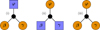 |
Fig. 1. Representations of isolated resonant three-mode coupling networks for modes φ, β and γ. They represent direct resonances (i), parametric resonances (ii), and driven resonances (iii). A linearly unstable (i.e., excited) mode is pictured as an orange circle, whereas a linearly stable (i.e., damped) mode is pictured as a blue square. |
In addition to these three isolated resonant coupling networks, non-isolated resonant coupling networks exist, in which a daughter or parent mode is shared among different resonantly coupled mode triads. O’Leary & Burkart (2014) called this multiple-mode or multi-mode coupling (see also e.g., Guo 2021). The selection rules derived in Sect. 2.4 remain valid in such networks, because coupling occurs at the same quadratic order. Networks with granddaughter and great-granddaughter modes have also been constructed. The reader is referred to Kumar & Goodman (1996) and Weinberg et al. (2021) for additional information on such networks.
Higher-order coupling terms, such as those that appeared in the cubic four-wave coupling networks developed to describe four interacting modes in non-rotating stars (by for example Van Hoolst & Smeyers 1993 and Van Hoolst 1994a) do not adhere to the selection rules in Sect. 2.4. The four-wave selection rules can however be determined from similar arguments. For example, the four-wave azimuthal selection rule was derived in Weinberg (2016). They however used the complex conjugate of mode φ in their definition of the mode coupling coefficient and did not expand in pairs of complex conjugates (as in Eq. (17)). This yielded a slightly different formulation of the azimuthal selection rule than what would be obtained for a coupling coefficient defined in a similar way as in Eq. (22).
A priori, it is not clear whether multi-mode or higher-order coupling terms are necessary to explain the (stationary) amplitudes and phases of the three-mode resonance candidate couplings detected among the modes of SPB stars analyzed in V21. The most parsimonious models for these identified candidate couplings would be isolated three-mode sum-frequency coupling networks that produce stable stationary solutions, if those solutions effectively describe observed (time-independent) amplitudes, phases and frequencies. We limit ourselves in the remainder of this work to describing such coupling networks.
2.6. Amplitude equations for Ω1 ≃ Ω2 + Ω3
Under the assumption that the linear driving or linear damping rate γφ of a mode φ fulfills |γφ/Ωφ|≪1 for the modes that are weakly non-linearly coupled, we can derive the AEs. In this section we use the coupled-mode Eqs. (20) and (21) valid for quadratically non-linear oscillations in rotating stars to derive the specific AEs for the sum-frequency resonant interaction Ω1 ≃ Ω2 + Ω3 between three distinct modes. Similar AEs were derived for the resonant harmonic interaction Ω1h ≃ Ω2h (with subscript h denoting the harmonic nature of the resonance) in Appendix B.2 of Van Beeck (2023). The AEs derived in this Section also describe the temporal evolution of the coupled mode’s properties of difference-frequency resonances Ω1d = Ω2d − Ω3d, as we show in Appendix F.
Following Van Hoolst (1995), we apply the multiple time scales perturbation method (e.g., Nayfeh 1973, 1981; Nayfeh & Mook 1979) to compute the mode amplitudes due to non-linear coupling at the quadratic level. We introduce time variables
 (26)
(26)
where 𝔍 is a small, dimensionless ordering parameter. The time derivative in Eq. (20) becomes
 (27)
(27)
The multiple time scales method then searches for an approximate solution for the complex amplitudes cφ of mode φ as
 (28)
(28)
Perturbation series (28) needs to be uniform: each of the higher-order terms should be a small correction to lower-order terms.
Substituting expansions (27) and (28) into the coupled-mode equations (20), subsequently dividing by the non-zero parameter 𝔍 and keeping terms up to first order in 𝔍, yields
 (29)
(29)
We examine this equation order by order in 𝔍 to determine the complex amplitude variation of the eigenmode φ in the form of AEs. The (linear) equation at order 𝔍0 is
 (30)
(30)
in which we introduce the linear operator Lφ as the mapping Lφ: ℂ → ℂ defined as ![Mathematical equation: $ L_{\varphi} (c) = \left({\frac{\partial }{\partial t_0}} + i\, \Omega_{\varphi}\right)[c] $](/articles/aa/full_html/2024/07/aa48369-23/aa48369-23-eq56.gif) for a complex amplitude c. The solution of Eq. (30) is
for a complex amplitude c. The solution of Eq. (30) is
 (31)
(31)
where aφ is a complex amplitude factor that varies only on time scales slower than the time scale t0 for each mode φ.
The equation at order 𝔍 is
 (32)
(32)
Substituting the linear solution (31) into Eq. (32) yields
 (33)
(33)
Some of the terms in the solution of Eq. (33) increase linearly in time. Such terms are called secular terms (e.g., Nayfeh 1973, 1981 and Nayfeh & Mook 1979) and must vanish to ensure we obtain a uniformly valid perturbation series.
Setting the terms that generate the secular terms in the solution of Eq. (33) equal to zero yields the AEs for the mode amplitudes and phases. These secular-term-generating terms have a multiplying factor exp(−iΩφt0) in Eq. (33), as shown in Appendix B.1 of Van Beeck (2023). The first term on the right side of Eq. (33) always generates a secular term. We obtain additional terms that generate secular terms by substituting the resonance condition Ω1 ≃ Ω2 + Ω3, defined in terms of the detuning parameters δω and ΔΩl,
 (34)
(34)
in Eq. (33). The condition that ensures that the sum of these secular-term-generating terms vanishes leads to the (extended complex) AEs for the sum-frequency resonance Ω1 ≃ Ω2 + Ω3:
 (35)
(35)
in which we introduce the linear growth or linear damping rates γφ for mode φ (e.g., Van Hoolst 1995) and use Eq. (22) to convert  into
into  (and similar). In Eq. (35), we also introduce the symbol ‘°’, which denotes a Hadamard-Schur (i.e., element-wise, Bhatia 2007; Bernstein 2009) product. We use the vectors
 (36)
(36)
and
 (37)
(37)
in Eq. (35). In Eq. (37), we define the isolated three-mode coupling coefficient η1:
 (38)
(38)
which respects the symmetry of coupling coefficient (22) under permutation of its indices. For exact resonances (i.e., δω = 0), the AEs reduce to a set of trivial equations. In such situations, efficient non-linear energy transfer is expected, and one enters the regime of intermediate to strong non-linear coupling, whereas the AEs are valid for weak coupling only.
By introducing real amplitudes Aφ and phases ϕφ as aφ = Aφexp(i ϕφ) with φ ∈ ⟦3⟧, where ⟦u⟧ denotes the set of integers { x∈ℕ0 | x≤u }, and separating the real and imaginary parts of the extended complex AEs (35), we obtain
 (39a)
(39a)
 (39b)
(39b)
where η1 = |η1| e−i δ1, and
 (40)
(40)
In the AEs (39) we also introduce the generic phase coordinate
 (41)
(41)
which contains the combination phase Φ = ϕ1 − ϕ2 − ϕ3. Because the coupling coefficients (22) do not depend on time, we have
 (42)
(42)
for non-zero resonant mode amplitudes, because of Eq. (39a) and the definition γ⊞ ≡ γ1 + γ2 + γ3. Equations (39a) and (42) thus form an autonomous four-dimensional system equivalent to the six-dimensional system in Eqs. (39a) and (39b), in which the individual mode phases ϕ1, ϕ2 and ϕ3 do not explicitly appear.
Non-linear interactions lead to non-linear frequency shifts, which can be derived from Eq. (39b) for the individual mode phases. By integrating these equations, the first order solution (31) can be expressed as
 (43)
(43)
in which the symbol ‘⊘’ denotes a Hadamard-Schur (element-wise) division, and where
 (44)
(44)
The third term in the exponential factor of Eq. (43) defines the quadratic non-linear frequency shift multiplied with the elapsed time. If the linear angular mode frequency in the co-rotating frame – the second term in that factor – is added to the non-linear frequency shift, we obtain a shifted frequency, hereafter referred to as the non-linear frequency, in the same reference frame. The expression for the (second-order) non-linear correction to the complex amplitude, cφ2, can be found in Appendix B.1 of Van Beeck (2023). The harmonic resonance equivalents of the non-linear frequency shifts and second-order non-linear corrections to the complex amplitudes can be found in Appendix B.2 of that work.
2.7. Stationary solutions of the amplitude equations
The candidate resonant three-mode couplings identified by V21 are time-independent, with the modes in a non-linear frequency (and phase) lock (i.e., they are synchronized). We therefore derive the time-independent or stationary solutions of the AEs (i.e., the fixed points of Eqs. (39a) and (42)) in this section.
The trivial stationary solution As = 0, in which the superscript ‘s’ denotes the stationarity of a quantity, is not oscillatory, and therefore cannot explain the observed couplings. From Eq. (39a), we obtain a oscillatory stationary solution,
 (45)
(45)
in which we define the stationary phase coordinate Υs as
 (46)
(46)
with  . The stationary equivalent of Eq. (42) yields an expression for the detuning parameter of stationary solutions,
 (47)
(47)
by setting  and
and  . To derive this equation, we assume that Υs ≠ p π (p ∈ ℤ). If Υs = p π, we retrieve the trivial solution, due to Eq. (45).
By considering the products of two equations of the three in Eq. (45), and using Eq. (47), we write the squared stationary amplitudes as
![Mathematical equation: $$ \begin{aligned} \left(\boldsymbol{A}^s\right)^{\circ 2} = \dfrac{\boldsymbol{Q}}{4\,|\eta _1|^2}\left[1 + q^2 \right]\,, \end{aligned} $$](/articles/aa/full_html/2024/07/aa48369-23/aa48369-23-eq80.gif) (48)
(48)
where the superscript ‘°n’ indicates a Hadamard-Schur (element-wise) nth power. In Eq. (48), we use the detuning-damping ratio q and quality factor vector Q, which we define as
 (49)
(49)
with quality factor Qφ ≡ Ωφ/γφ for φ ∈ ⟦3⟧. The resonant stationary amplitudes are real if
 (50)
(50)
for a driven resonance scenario, or if
 (51)
(51)
for direct and parametric resonance scenarios. In Eqs. (50) and (51), ΩN and ΩP are the mode frequency variants of the vectors AN and AP defined in Eq. (40). The operators > ° and ∈° are the element-wise equivalents of the operators > and ∈. Equivalent expressions describing stationary solutions for harmonic resonances can be found in Appendix B.2 of Van Beeck (2023).
Three quantities determine the stationary mode amplitudes: the non-linear interaction described by coupled-mode Eqs. (20) and (21), the linear eigenmode properties given by Q, and the detuning of the resonance measured by q. For decreasing values of the non-linear coupling coefficients |η1|, the efficiency for non-linear energy transfer between modes is lower, hence, the stationary amplitudes (48) become larger, because a larger mode energy (and thus mode amplitude) is required to transfer enough energy in order to have a significant non-linear effect leading to amplitude saturation. Quality factor Qφ expresses the ratio of the mode φ’s e-folding damping or driving time ( ) relative to its angular period (
 ). With increasing |Qφ|, more mode periods are needed for the mode energy (normalized to GM2/R) to damp or grow by a factor of e due to linear heat-driven damping or driving. The stationary amplitude of a certain mode therefore decreases if the other modes involved in the triad have larger values of |Qφ|, because then either a linearly (heat-)driven mode φ gains less energy per cycle or a linearly (heat-)damped mode φ loses energy more slowly per cycle. For example, in the parametric resonance scenario, the stationary amplitude of the daughter mode 2 or 3 is increased when the parent mode is driven faster (by the κ mechanism) and when the other daughter mode 3 or 2 is damped faster. The stationary amplitude of the parent mode 1 is larger when it is coupled to daughter modes that are more difficult to non-linearly excite (i.e., a larger parent mode energy is required to have a measurable non-linear effect).
Increasing values of |q| lead to increasing values of the stationary amplitudes. Two factors affect the value of the detuning-damping ratio q: the detuning δω and γ⊞ (≡γ1 + γ2 + γ3). For larger detunings the stationary amplitudes increase, because the increased detuning reduces the efficiency of the non-linear mode coupling (similar to decreasing |η1|), requiring a larger amplitude for a non-linear effect. For smaller values of |γ⊞|, that is, for the case where the parent and daughter mode linear heat-driven growth and damping rates almost balance out, there is very weak overall linear excitation or damping, requiring a very close resonance (i.e., small detuning) and large amplitudes to have a non-linear effect.
The relative stationary energies of the modes in the triad are related by the ratios of their quality factors, assuming conditions (50) or (51) hold:
 (52)
(52)
The energy ratios (52) do not depend on the non-linear coupling coefficients because of the symmetry of these coefficients, and are determined by linear properties of the modes only. Therefore, of two linearly damped modes, the one with the longest damping time per cycle (largest |Qφ|) reaches the largest stationary amplitude through non-linear energy transfer from the linearly excited mode, because it loses energy more slowly.
Non-linear stationary frequencies Ωnl, s for modes φ ∈ ⟦3⟧ are obtained from Eq. (43) in the form
 (53)
(53)
with the non-linear stationary frequency shifts  given by
 (54)
(54)
to first order. For parametric and direct resonance scenarios, the sign of the frequency shift is thus determined by the sign of ΔΩl. The non-linear stationary frequencies  are frequency-locked, meaning that they satisfy the resonance condition (34) exactly:
 (55)
(55)
which follows from Eq. (46) and  . Explicit expressions for harmonic resonance frequency shifts can be found in Appendix B.2 of Van Beeck (2023). As stated in Sect. 2.6, the derived stationary quantities in this Section also describe the stationary properties of modes in difference-frequency resonances.
2.8. Stability of the stationary amplitude equation solution
From a mathematical perspective, the system of amplitude equations defined by Eqs. (39a) and (42) is an autonomous dynamical system, and its stationary solutions are fixed points of that dynamical system. One of the fundamental results of dynamical systems theory is the Hartman-Grobman or linearization theorem, which states that if a fixed point is hyperbolic, a linearization of the dynamical system can be used to trace the asymptotic behavior of dynamical system solutions near the fixed point (Guckenheimer & Holmes 1983; Betounes 2010). The stability of a hyperbolic fixed point can thus be determined from the linearization of the system around that point. Two conditions need to be fulfilled for a fixed point  of a dynamical system
  to be hyperbolic: both the Jacobian and the real parts of the eigenvalues of the Jacobian matrix of
  cannot be equal to zero (Guckenheimer & Holmes 1983; Betounes 2010). Hereafter, we collectively refer to these two conditions as the hyperbolicity condition. The Jacobian matrix of a dynamical system of amplitude equations depends on the values of the respective non-linear coupling coefficients because the hyperbolicity condition considers the geometry of the non-linear solution around the fixed point (see Appendices B.1 and B.2 of Van Beeck 2023 for the expressions).
In the remainder of this section we assume that the hyperbolicity condition is fulfilled for the stationary solution, so that a linearization can be used to guarantee the stability of that solution. Let us now examine the stability of the stationary solutions for each of the three isolated resonant coupling scenarios discussed in Sect. 2.5. Physically, the stability of the (hyperbolic) stationary solutions of the AEs is governed by the reaction of the system (i.e., the pulsating star) to small disturbances away from the stationary state (in this case, away from the stationary pulsation solution). Such disturbances can be damped or get amplified over time. If they are damped, the stationary solution is stable. The solution is unstable if they get amplified.
To derive the linearized dynamical system, we introduce small perturbations of the stationary amplitudes (δAφ for mode φ) and phases (δϕφ for mode φ), so that the complex amplitudes take the form (Van Hoolst 1995)
![Mathematical equation: $$ \begin{aligned} a_{\varphi } = \left(A^s_{\varphi } \,+\, \delta A_{\varphi }\right) \exp \left[i\left(\phi _{\varphi }^s \,+\, \delta \phi _{\varphi }\right)\right], \forall \, \varphi \in [\![3]\!]\,. \end{aligned} $$](/articles/aa/full_html/2024/07/aa48369-23/aa48369-23-eq96.gif) (56)
(56)
Substituting the perturbed complex amplitude factor (56) into the complex-valued AEs (35), subsequently linearizing and separating the real-valued and complex-valued parts, yields the tensor equation that describes the time evolution of the perturbations,
 (57)
(57)
Here, M is the stability matrix, defined as
 (58)
(58)
and Z is the perturbation tensor defined as
 (59)
(59)
for which
![Mathematical equation: $$ \begin{aligned} \delta \Upsilon = \delta \phi _1 - \delta \phi _2 - \delta \phi _3\,, \gamma _{\boxplus _\varphi } \equiv \gamma _\boxplus - 2\,\gamma _\varphi , \forall \varphi \in [\![3]\!]\,. \end{aligned} $$](/articles/aa/full_html/2024/07/aa48369-23/aa48369-23-eq100.gif) (60)
(60)
We infer an analytical stability domain of the stationary solutions of the AEs based on the Routh-Hurwitz stability criterion (e.g., Hahn 1967; Cesari 1971; Kubicek & Marek 1983). Necessary but not sufficient conditions for stability are that the Hurwitz determinants Hu are positive (see Appendix B.4 in Van Beeck 2023):
 (61a)
(61a)
 (61b)
(61b)
 (61c)
(61c)
 (61d)
(61d)
in which the coefficients wu (u ∈ ⟦4⟧0, with ⟦n⟧0 ≡ {0} ∪ ⟦n⟧ = { x∈ℕ | x≤u }) are the coefficients of the characteristic polynomial pZ(λ) of the stability matrix (58),
 (62)
(62)
In Eq. (62), λ denotes an eigenvalue of the tensor Eq. (57), and the coefficients wu are
 (63a)
(63a)
 (63b)
(63b)
![Mathematical equation: $$ \begin{aligned} { w}_2 =&\, \gamma ^2_\boxplus \left[1 + q^2\right] -4\,q^2\,\left[\gamma _1\,\gamma _2 + \gamma _1\,\gamma _3 + \gamma _2\,\gamma _3\right]\,,\end{aligned} $$](/articles/aa/full_html/2024/07/aa48369-23/aa48369-23-eq108.gif) (63c)
(63c)
![Mathematical equation: $$ \begin{aligned} { w}_3 =&\, 4\,\gamma _1\,\gamma _2\,\gamma _3\, \left[1 + 3\,q^2\right]\,,\end{aligned} $$](/articles/aa/full_html/2024/07/aa48369-23/aa48369-23-eq109.gif) (63d)
(63d)
![Mathematical equation: $$ \begin{aligned} { w}_4 =&\, -4\, \gamma _\boxplus \, \gamma _1\,\gamma _2\,\gamma _3\, \left[1 + q^2\right] \,. \end{aligned} $$](/articles/aa/full_html/2024/07/aa48369-23/aa48369-23-eq110.gif) (63e)
(63e)
These are the same coefficients as the ones that were determined by Dziembowski (1982) in his formalism for quadratic non-linear mode coupling of three distinct modes in non-rotating stars. Because H3 > 0 due to the stability condition (61c), stability condition (61d) becomes w4 > 0.
The necessary but not sufficient stability conditions in Eq. (61) show that a stationary solution at the quadratic coupling level is always unstable for the driven resonant coupling scenario, because Eq. (61a) and γ> °0 are contradictory. This is a logical consequence of only considering modes that are linearly excited and can exchange energy between them, and not including third-order couplings that can limit the amplitude. The direct resonant three-mode coupling scenario also always yields unstable stationary solutions for distinct modes 2 and 3, similar to what was found by Dziembowski (1982), because Eqs. (61a) and (61d) contradict each other if the necessary stability condition (61c) is to be satisfied. Hence, driven and direct resonance scenarios lead to time-variable amplitudes for their coupled modes. Modes in such coupling scenarios can for example lead to limit cycle behavior of the amplitudes (see e.g., Seydel 2009). For the parametric resonant three-mode coupling scenario, Eq. (61d) is trivially fulfilled if Eqs. (61a) and (61c) are fulfilled. The stability of the fixed points of harmonic resonance analogues is discussed in Appendix B.2 of Van Beeck (2023).
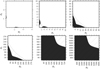 |
Fig. 2. Stability domains as a function of ϑ2 and ϑ3, indicated by the dark, shaded area, and evaluated using Eqs. (61a) and (64) for different values of |q1|. Specifically, |q1| is set equal to 0.1 (left top panel), 1 (middle top panel), 10 (right top panel), 102 (left bottom panel), 103 (middle bottom panel) and 104 (right bottom panel). The stability domain determined by the stability conditions defined in Dziembowski (1982) is larger and is also indicated in these panels by the hatched areas. Unhatched white areas of the figure panels indicate unstable domains. Note the different axis scales for the different panels, which indicates the importance of the value of |q1| in determining the stability of stationary solutions. |
In addition to Eq. (61), all wu also need to be positive to obtain stable parametric stationary solutions (see e.g., Hahn 1967 and Appendix B.4 in Van Beeck 2023). Combining these additional conditions with Eq. (61), the stability domain of a parametric three-mode resonant coupling with real amplitudes can be described by only three conditions: Eq. (61a), the hyperbolicity check, and the quartic condition
![Mathematical equation: $$ \begin{aligned} \dfrac{-\gamma _1^3}{\gamma _\boxplus }\left[\mathfrak{d} _4 + \mathfrak{d} _2\, q^2 + \mathfrak{d} _0\, q^4\right] > 0\,\, \Leftrightarrow \,\, \mathfrak{d} _4 + \mathfrak{d} _2\, q^2 + \mathfrak{d} _0\, q^4 > 0\,. \end{aligned} $$](/articles/aa/full_html/2024/07/aa48369-23/aa48369-23-eq111.gif) (64)
(64)
The factor  in Eq. (64) is positive for parametric resonances that fulfill Eq. (61a). The dimensionless quartic coefficients 𝔡u (u = 0, 2, 4) in that equation are given by
![Mathematical equation: $$ \begin{aligned}&\begin{aligned}\mathfrak{d} _0 =&\, -18\,\vartheta _2\vartheta _3 - 3 \left(1 -\vartheta _2 - \vartheta _3\right)\\&\left[\left(1 -\vartheta _2 - \vartheta _3\right)^2 + 4\left(\vartheta _2 + \vartheta _3 - \vartheta _2\vartheta _3\right)\right]\,,\end{aligned}\end{aligned} $$](/articles/aa/full_html/2024/07/aa48369-23/aa48369-23-eq113.gif) (65a)
(65a)
![Mathematical equation: $$ \begin{aligned}&\begin{aligned}\mathfrak{d} _2 =&\, -12\,\vartheta _2\vartheta _3 - \left(1 -\vartheta _2 - \vartheta _3\right)\\ &\left[2 + \left(\vartheta _2 - \vartheta _3\right)^2 + \left(\vartheta _2 + \vartheta _3\right)^2\right]\,,\end{aligned}\end{aligned} $$](/articles/aa/full_html/2024/07/aa48369-23/aa48369-23-eq114.gif) (65b)
(65b)
 (65c)
(65c)
where we define ϑ2, 3 ≡ −γ2, 3 / γ1, which are positive for parametric resonances. The physical meaning of these dimensionless ratios is similar to that of the quality factor ratios discussed in Sect. 2.7, but inverse: they compare the damping and/or driving time scales.
The quartic stability condition (64) is symmetric in ϑ2 and ϑ3, in accordance with the symmetry of the coupling coefficient. Coefficients 𝔡2 and 𝔡4 are the same as in Eq. (6.14) of Dziembowski (1982). Although the coefficient 𝔡0 differs from the one given in that equation, likely due to an error in Dziembowski (1982), the stability condition is derived from the same characteristic polynomial coefficients defined in Eq. (63). The coefficients 𝔡u (u = 0, 2, 4) are a function of ϑ2 and ϑ3 only, whereas q can be expanded as a function of ϑ2, ϑ3, and the ratio of the linear frequency detuning to the parent’s linear driving rate q1 ≡ δω/γ1. We therefore can explore the stability domain of the (hyperbolic) stationary solutions by varying only three dimensionless ratios of linear variables: q1 = δω/γ1, ϑ2 and ϑ3. The dimensionless ratio q1 can be written as
 (66)
(66)
where the cyclic co-rotating frame period P1 = 2 π / Ω1. It is therefore a period-weighted combined measure of the driving time scale of the linearly excited parent mode (Q1) and the efficiency with which non-linear energy transfer occurs (δω). Hence, when comparing values of q1 for triads with linearly excited modes of similar period, one might expect that the triad with larger |q1| has larger stationary mode amplitudes because of decreased efficiency of non-linear energy transfer (larger δω) and/or smaller stationary mode energy ratios  (larger Q1, when values of Q2, 3 are comparable).
Figure 2 displays the domains of stability of stationary solutions in the three-dimensional phase space of the parameters q1, ϑ2 and ϑ3, covering commonly encountered parameter values when modeling mode interactions in SPB stars (see Sect. 4.3). The necessary condition (61a) for stability of the fixed point, which requires that ϑ2 + ϑ3 > 1, is clearly recognizable on the left and middle panels in the top row of Fig. 2. Physically, this expresses that daughter modes must be sufficiently damped compared to the linear excitation of the parent mode for stability, otherwise, resonant energy transfer will increase all amplitudes without bound.
The quartic stability condition (64) is more difficult to interpret. Term (1 − ϑ2 − ϑ3) in that stability condition is always negative due to Eq. (61a) and can be interpreted as an effective total-damping-to-linear-driving ratio γ⊞/γ1. If the absolute value of the ratio is large, the overall damping per unit of driving is large as well. Other terms are less straightforward to interpret. Hence, we base our interpretation of this stability condition primarily on the stability domains pictured in Fig. 2. The quartic stability condition derived in this work is stricter than that of Dziembowski (1982) (displayed as hatched areas in Fig. 2) due to the difference in value of the coefficient 𝔡0. Condition (64) can also be expressed in terms of q1, ϑ2 and ϑ3. Hence, conclusions drawn from the visualized stability domains in the chosen phase space (shown in Fig. 2) can be related to the equivalent stability condition that is expressed in terms of these three variables.
For large values of ϑ2 and ϑ3 a regime of strong damping (relative to the linear excitation of the parent mode) is reached. In such strong damping regimes the fixed point solutions are unstable because the transfer of energy (per cycle) is not enough to overcome linear damping. The domain of stability at the strong damping end of the ϑ2 − ϑ3 plane moves towards larger values of ϑ2 and ϑ3 for larger values of q1, as shown in the different panels of Fig. 2. Conversely, the stability domain decreases considerably in size for smaller values of q1. This can be explained by an increase (decrease) in energy transfer efficiency and/or an increase (decrease) in energy available for transfer, leading to faster (slower) rates of energy transfer and corresponding smaller (larger) domains of stability, based on the physical explanation of Eq. (66). Specifically, for faster (slower) rates of energy transfer per cycle, the stationary solutions can endure smaller (larger) perturbations around the stationary solutions before energy transfer renders the fixed points unstable. The stability of the stationary solutions is thus primarily determined by the speed of energy transfer.
2.9. The onset of parametric instability
In this section we derive the minimum amplitude conditions for the onset of the parametric resonance instability for the non-linear interaction among three distinct modes in a sum or difference frequency. If this instability does not occur for these three distinct modes, the amplitudes of the modes in the triad can only be limited to stable stationary values by higher-order non-linear mode coupling terms, such as the cubic self-coupling terms that were described in Van Hoolst (1996). Alternatively, limit cycles characterized by non-stationary amplitudes may occur. Similar conditions for the onset of parametric and direct resonant instability derived for harmonic resonances can be found in Appendix B.2 of Van Beeck (2023).
The initial growth of the daughter modes can be described using the complex AEs (35) for one of the daughter modes and its complex conjugate for the other daughter mode. If we then set ak = Sk exp(−i δω t1/2) (for k ∈ {2 , 3}, following Dziembowski 1982) the explicit time-dependence disappears. Further assuming that the complex amplitude factor a1 stays constant, a plausible assumption in the initial phase of energy transfer, yields
 (67a)
(67a)
 (67b)
(67b)
Under the assumption that Sk ∼ exp(σ t1) (for k ∈ {2,3}), Eq. (67) can be solved for the growth parameter σ, yielding
 (68)
(68)
equivalent to expressions given by Vandakurov (1981) and Dziembowski (1982). Parametric instability will occur if Re[σ] > 0, because this ensures growth of the daughter mode amplitudes A2 and A3. At the onset of parametric instability, Re[σ] = 0. We therefore define the instability threshold amplitude for the parent mode At as the value of A1 for Re[σ] = 0. The growth parameter σ is then imaginary and we can set σ = p i, with p determined by solving Eq. (68):
 (69)
(69)
Using this expression in the real part of the growth parameter (68) yields the parametric instability threshold amplitude
 (70)
(70)
Instability threshold amplitude (70) is equivalent to the ones derived in Dziembowski (1982), Wu & Goldreich (2001) and Arras et al. (2003).
Parametric resonant mode triad interactions require that the parent mode amplitude A1 ≥ At, and  is always larger than At. In the limit of very small (non-zero) detuning δω, the threshold amplitude is solely dependent on the coupling coefficient and the quality factors. In that case, At increases with decreasing |η1| and faster damping of the daughter modes (expressed by the quality factors) because both terms limit the amplitude growth of the daughter modes due to non-linear energy transfer, thus requiring a larger parent mode energy for a visible non-linear effect. A larger detuning increases the threshold amplitude because of the less efficient energy transfer.
3. Theoretically predicted observables
An important observable in linear g-mode asteroseismic modeling is a g-mode period spacing pattern (which are extensively described in the literature; see e.g., Aerts et al. 2018; Michielsen et al. 2021; Bowman & Michielsen 2021 for some recent examples of how they can be used to probe internal mixing). In this section we derive additional observables based on the theoretical AE formalism described in Sect. 2 and outline how to compare them to observed quantities.
An inherent assumption of our models is that the modes are coherent. That assumption is justified because the detected frequencies of variability in SPB stars have been observed to be stable with a frequency precision of order 10−7 d−1, based on long-term ground-based photometric monitoring (De Cat & Aerts 2002). This is not necessarily the case for other pulsators: δ Sct stars, for example, show frequency and amplitude modulation in the majority of detected signals (Bowman et al. 2016). Amplitude and frequency modulation also occurs among g mode triplets in oscillating white dwarfs (see e.g., the pioneering study of the oscillating DB white dwarf star KIC08626021 by Zong et al. 2016b). Moreover, the amplitudes of the oscillating hot B subdwarf star KIC10139564 reveal that the modulation of its observed p modes is larger than that of its g modes (Zong et al. 2016a). Whether this trend is generic among oscillating stars remains to be verified.
3.1. Amplitudes: model-generated luminosity fluctuations
We cannot compare the theoretical stationary amplitudes derived in Sect. 2.7 with the surface luminosity amplitudes  determined from observations. These theoretical stationary amplitudes must first be converted to the corresponding observables, the theoretical luminosity fluctuations at the stellar surface, 𝔏.
In this section we follow the approach of Fuller (2017) to compute a conversion factor oA used to convert a theoretical amplitude into a theoretical luminosity fluctuation 𝔏 caused by an oscillation mode of a resonant triad. Analogous to Eq. (82) in Fuller (2017), we estimate the disc-averaged luminosity fluctuation for a single SPB star due to g mode φ as
 (71)
(71)
within the TAR, where
 (72)
(72)
in which ΔLφ, R(R) is the Lagrangian surface luminosity perturbation due to mode φ, ξφ, r is the radial part of the adiabatic eigenfunction of that mode, is is the angle between the rotation axis and the line of sight at time t = 0 s (also called the spin inclination angle, see e.g., Fuller & Lai 2012), and tk and ek are limb-darkening coefficients given by the overlap integrals (in analogy to e.g., Burkart et al. 2012)
 (73a)
(73a)
![Mathematical equation: $$ \begin{aligned} e_k&= \int _0^1\left[2\,\mu ^2\,\frac{\mathrm{d}H_r(\mu ; k)}{\mathrm{d}\mu } - \left(\mu - \mu ^3\right)\frac{\mathrm{d}^2H_r(\mu ; k)}{\mathrm{d}\mu ^2}\right]\,h(\mu )\,\mathrm{d}\mu \,, \end{aligned} $$](/articles/aa/full_html/2024/07/aa48369-23/aa48369-23-eq128.gif) (73b)
(73b)
where μ ≡ cosθ and h(μ) is a limb-darkening function. To derive Eq. (71), we assume that the Lagrangian flux perturbation of mode φ, which causes the luminosity perturbation, is equal to the radiative flux perturbation (see e.g., Unno et al. 1989). We use a linear limb-darkening function h(μ)=1 + (3 μ/2) in our computations (as has been customary for decades; see e.g., Osaki 1971 and Aerts et al. 1992, who set μ = 0.36 for B stars). One can however easily account for other, more sophisticated limb-darkening laws by changing the limb-darkening function. Numerical evaluations of tk and ek are necessary, because no analytic closed forms of the classical Hough functions exist.
Equation (71) thus separates contributions to the disc-averaged luminosity fluctuation (ΔLφ / L) into two multiplicative factors: a factor attributed to the properties of the mode φ under consideration, (ΔLφ / L)mode, and an angular factor that describes the observer’s orientation in the rotating frame. The theoretical flux fluctuation of that mode at the surface, 𝔏φ, can then be computed by multiplying the (complex) amplitude cφ obtained from solving the AEs with the factor (ΔLφ / L). Its modulus |𝔏φ| can directly be compared with observed luminosity amplitudes  . The amplitude conversion factor oA, φ for a mode φ is then defined as
 (74)
(74)
We compute the expected theoretical threshold surface luminosity fluctuations |𝔏t|, which is the minimum observed luminosity fluctuation that a parent mode in a mode triads needs for (parametric) resonant mode coupling to occur, and the stationary surface luminosity fluctuation  of mode φ, as
 (75)
(75)
The theoretical g mode stationary amplitudes  and the theoretical g mode (parametric) threshold amplitudes At in Eq. (75) are computed by setting the bookkeeping parameter 𝔍 = 1 (similar to e.g., Buchler & Goupil 1984), so that δω = ΔΩl.
The conversion factors (74) are sensitive to the choice of a limb-darkening function (because this affects tk and ek), as well as the normalization factors for the Hough functions and the radial parts of the mode eigenfunctions defined in Eq. (11) and Sect. 2.3, respectively. The stationary daughter-parent surface luminosity ratios  ,
,  minimize the influence of the choice of limb-darkening function and normalization factors. We determine these ratios as
 (76)
(76)
The daughter-parent surface luminosity fluctuation ratios (76) are the most robust amplitude-based theoretically predicted observables that can be used in resonant non-linear asteroseismic modeling. To derive the expressions for these ratios, we assume a parametric resonant mode triad (for a three-mode sum-frequency coupling or its difference frequency analogue), and use the definition of the quality factor Qφ, in addition to Eq. (52). Stationary surface luminosity ratios can thus be computed in terms of linear non-adiabatic parameters. The equivalent expression for the daughter-parent surface luminosity fluctuation ratio of a harmonic dyad is given in Appendix B.2 of Van Beeck (2023).
In this work, we only envision a rough comparison between theoretical predictions and observables by limiting ourselves to monochromatic predictions. As highlighted by Aerts & Tkachenko (2023), future studies of measured amplitude ratios from multi-color space photometry by combining Gaia (Gaia Collaboration 2016), Kepler (Koch et al. 2010) or PLATO (Rauer et al. 2014) data offer additional opportunities to characterize stellar atmospheric properties. Concrete applications of our theory require integrations over particular passbands instead of the monochromatic predictions for the daughter-parent ratios considered here. Such integrations will not be considered in this work but will be considered in follow-up application papers.
3.2. Frequencies and phases: frequency detuning and combination phase for Ω1 ≈ Ω2 + Ω3
The inherent assumption made in linear asteroseismic inference is that any non-linear frequency shifts (e.g., those determined by Eq. (54)) are negligible, so that theoretical frequencies computed within a linear formalism can directly be compared to their observed counterparts. A non-linear formalism, such as the one we derive in Sect. 2, allows one to verify that assumption.
We define the observed frequency detuning  as
as
 (77)
(77)
where the observed frequencies of modes φ are defined as  with subscript 𝔦 indicating that observed frequencies are measured in the inertial frame. Because of the azimuthal selection rule (24),
  is also equal to its co-rotating frame equivalent
  , that is,
  . This equivalence, along with Eq. (55) and the stationary equivalent of Eq. (77), then determine that
 (78)
(78)
needs to be fulfilled for a isolated (resonantly locked) mode triad. In identifying such couplings observationally, one should therefore search for combinations of observed modes with stationary amplitudes, for which
 (79)
(79)
where  is the propagated uncertainty of
  , and
, and  denotes the Rayleigh limit, with T being the total time span of the time series of the SPB star that needs to be modeled.
The observable that can directly be compared with observed frequencies of modes in an inferred candidate resonance is
 (80)
(80)
which includes the quadratic stationary non-linear frequency shift (54). By summing 𝔏φ = oA, φ Aφ with its complex conjugate, we determine the individual stationary phase observables (see Sect. 4.3.2 in Van Beeck 2023 for the explicit manipulations)
 (81)
(81)
where we use the stationary equivalent of Eq. (39b), as well as Eqs. (34), (45), and (49). In Eq. (81), ϕL φ is the phase of the complex quantity (ΔLφ / L)mode defined in Eq. (72). The observed individual mode phases (81) therefore are independent of time if the modes are part of a locked mode triad.
In analogy with the definition of the stationary equivalent of the theoretical generic phase coordinate Υ in Eq. (41), we define the stationary combination phase observable  as
as
 (82)
(82)
where the last equality holds because of Eq. (81), and in which  and
and  . The coupling coefficient η1 is real-valued and therefore has no contribution to Eq. (82). Stationary combination phase observable (82) is to be compared with a relative phase computed from the phases of observed candidate resonance signals.
4. Numerical results for SPB models
We simulate stationary resonant parametric three-g-mode coupling processes by computing a grid of models representative for the SPB oscillators. Numerical stellar evolution models are generated by the stellar evolution code MESA (version 15140; Paxton et al. 2011, 2013, 2015; Paxton et al. 2018, 2019). Linear stellar oscillation models are generated by the stellar oscillation code GYRE (version 6.0.1; Townsend & Teitler 2013; Townsend et al. 2018; Goldstein & Townsend 2020), and use the MESA models as input. Numerical mode coupling models use both MESA and GYRE models as input.
We discuss the MESA model grid setup in Sect. 4.1, the GYRE model grid setup in Sect. 4.2, and display and discuss the numerical results for triad ensembles in Sect. 4.3. The link to our inlists for these codes, as well as the link to our mode coupling code repository, can be found in Appendix G.
4.1. MESA model grid setup for SPB stars
We compute MESA stellar evolution models with the parameters given in Table 1. These parameters cover the ranges of inferred initial mass (Mini) and core hydrogen mass fraction (Xc) values for SPB stars given in Table 2 of Pedersen (2022). The MESA models have the ‘standard’ initial chemical mixture of nearby B-type stars derived by Nieva & Przybilla (2012) and Przybilla et al. (2013), and an Eddington gray atmosphere. Following Pedersen et al. (2021), we adjust the initial hydrogen and helium mass fractions Xini and Yini so that the ratio  , with X* and Y* equal to the Galactic standard values for B-type stars in the solar neighborhood (Przybilla et al. 2013). We use Opacity Project (OP) opacity tables (Seaton 2005) that were computed by Moravveji et al. (2015) for this elemental mixture. The full proton-proton chain and CNO cycle nuclear reaction networks are used to describe core hydrogen fusion on the main sequence. Beyond the zero age main sequence (ZAMS), we use the Vink et al. (2001) hot wind scheme with a wind scaling factor fixed to a value of 0.3 (see Björklund et al. 2021).
Model parameters of the MESA model grid.
Diffusive isotope mixing processes within the stellar interior are assumed to be described by the simplified transport Eq. (1) of Michielsen et al. (2021) and Pedersen et al. (2021). Mixing processes in the radiative envelope are described by a diffusive mixing profile for internal gravity wave mixing deduced by Rogers & McElwaine (2017) and used by Pedersen et al. (2018) in the context of asteroseismic modeling. This profile scales the radiative envelope mixing level Denv with a factor inversely proportional to the (local) mass density. To model core-boundary mixing (CBM) processes, we employ an approach similar to the diffusive exponential overshooting model with efficiency parameters fCBM and f0 fixed to 0.02 and 0.005 (see e.g., Michielsen et al. 2019, 2021). The inner boundary of the overshooting zone (i.e., the convective core mass) is determined by the Ledoux criterion for mixing length parameter αMLT = 2.0 within the Cox & Giuli (1968) formalism for mixing length theory. In the implementation, we set the minimal level of diffusive isotope mixing Denv, min equal to 100 cm2 s−1. If the mixing level drops below that boundary at a certain location within the model, diffusive mixing is halted locally.
Our baseline (fiducial) model is a near terminal age main sequence (TAMS) model with Xc = 0.09, Mini = 4 M⊙, solar initial metallicity (Zini = 0.014), and fCBM equal to 0.02. Models ΔXc, 1 and ΔXc, 2 have core hydrogen mass fractions Xc equal to 0.29 and 0.59, respectively, and are representative for a mid-MS and near-ZAMS SPB star, because Xc is a proxy for the main sequence age of the star (hydrogen is depleted in the core during the main sequence). Model ΔXc|Mini is representative of a Mini = 6 M⊙ mid-MS SPB star. The fixed values of the parameters Denv, min, fCBM and Zini are representative of the median values of these parameters in Table 2 of Pedersen (2022).
To compute the non-linear quadratic mode coupling coefficients (22), we need the adiabatic derivative of Γ1 with respect to the stellar density,  . We compute this quantity in the MESA models with a custom function defined in Appendix C.2.
4.2. GYRE model grid setup for SPB stars
The most commonly observed g modes in SPB stars are prograde (k, m)=(0, 1) and (k, m)=(0, 2) modes (see e.g., Pedersen et al. 2021; Szewczuk et al. 2021). For each of the computed MESA models, we therefore compute the GYRE linear adiabatic and non-adiabatic eigenfrequencies and eigenfunctions of these commonly detected g modes, within the Cowling approximation (Cowling 1941) and the TAR. We assume uniform rotation at 20% of the Roche critical rotation rate ΩRoche for most models, except for the ΔXc, 2 model, for which we consider rotation at rates equal to 20% and (the excessively high) 60% of ΩRoche. The positive (negative) linear driving (damping) rates of the modes are estimated as the imaginary part of the non-adiabatic linear eigenfrequencies computed by GYRE.
Radial order ranges {nu} (u ∈ ⟦3⟧) of the (k, m)=(0, 2) parent and (k, m)=(0, 1) daughter modes computed with GYRE and based on the MESA models listed in Table 1, angular rotation rates Ω expressed in percentages of the Roche critical rotation rate ΩRoche and in d−1, model radius R, and the order of magnitude of the bounds for the ranges of ϑ2 and ϑ3 (denoted by ϑ2, 3), q1 and the quality factors Qφ (φ ∈ ⟦3⟧).
The radial orders of the g modes computed for the different MESA stellar evolution models are listed in Table 2. These are similar to those of Pedersen et al. (2021). We ensure that the linear non-adiabatic GYRE computations – which use trial frequencies based on the adiabatic GYRE computation results – do not show evidence of missing non-adiabatic mode radial orders (see e.g., Goldstein & Townsend 2020), so that there is a one-to-one mapping between the adiabatic and non-adiabatic mode radial orders. The ranges for the quality factors in Table 2 show that the condition |γφ/ωφ|≡|1/Qφ|≪1 mentioned in Sect. 2.6 is fulfilled for all modes (i.e., all modes are on the slow manifold).
4.3. Search for isolated mode couplings: triad parameter ensembles for SPB stars
Following the stability analysis in Sect. 2.8, only parametric resonance scenarios are able to produce stable stationary solutions for resonances Ω1 ≈ Ω2 + Ω3 (or their difference frequency analogues). We therefore restrict the GYRE computations of potential parent modes to those (k, m)=(0, 2) modes with linear driving rates γ1 > 0, and restrict the computations of potential daughter modes to those (k, m)=(0, 1) modes with linear damping rates γ2 < 0 and γ3 < 0. Gaps in the daughter mode radial order ranges {n2, 3} listed for some of the models in Table 2 indicate the presence of linearly excited (k, m)=(0, 1) modes that cannot partake in a parametric resonance. For the 6 M⊙ near-ZAMS and 8 M⊙ mid-MS and near-ZAMS models with a rotation rate of 20% of ΩRoche, we obtain no linearly excited potential parent modes.
We compute mode coupling coefficients η1 for mode triads whose stationary AE solutions satisfy the (linear) stability conditions derived in Sect. 2.8. To guarantee non-linear stability of the stationary solutions, these mode triads also need to fulfill the hyperbolicity check. This hyperbolicity check can only be done after performing the non-linear mode coupling computations, because the computed stationary Jacobian matrix contains the coupling coefficient |η1| (see Eq. (B.39) in Van Beeck 2023). The additional model validity constraints discussed in the next subsection are implemented to ensure that the solutions are away from the edge of the domains of applicability.
4.3.1. Model validity criteria
Buchler et al. (1997) state that resonant AEs are valid not only near a resonance center, but also far from resonance, with the solutions from resonant AEs slowly approaching the non-resonant AE solutions when moving away from that resonance center. This point however only holds under the assumption that all modes participating in the modal coupling are linearly unstable, so that a stable multi-mode fixed point is reached with the same modes for resonant and non-resonant AEs (Buchler et al. 1997). If that were not the case, the non-resonant solutions would predict negligibly small amplitudes for linearly damped modes. For the cubic couplings considered by Buchler et al. (1997), stable stationary points might exist for the driven resonance scenarios required for this type of behavior. However, for the quadratic non-linear couplings considered in this work, stable multi-mode fixed points can only be found for parametric or direct resonant scenarios (with the latter only yielding stable stationary solutions for harmonic resonances; see Sect. 2.8). Linearly damped modes participate in such coupling scenarios, invalidating the Buchler et al. (1997) assumption.
The resonant AEs derived in Sect. 2.6 are therefore valid only near the resonance center, that is, if the absolute value of the linear triad frequency detuning ΔΩl defined in Eq. (34), is small in comparison to the absolute values of the individual co-rotating-frame mode frequencies: |ΔΩl|≪|Ωφ| ∀φ ∈ ⟦3⟧. If it is not small, there are no comparatively slow amplitude variations and additional mode interactions need to be considered to describe the dynamics. We therefore estimate the validity domain of the AEs in terms of the parameter:
 (83)
(83)
which compares |ΔΩl| with the minimum absolute value of the co-rotating-frame angular mode frequencies of the triad. We require that mode triads considered for modeling have ΨAE ≤ 0.1, so that |ΔΩl| ≪ |min(Ω1, Ω2, Ω3)|. Many mode triads satisfy this model validity criterion, as is shown in Table 3.
Overview of the number of mode triads that satisfy different model validity and stability criteria.
It is furthermore important to consider the threshold surface luminosity fluctuations |𝔏t| of all possible mode triads, because these determine the onset of mode interaction. To obtain isolated mode couplings, we determine the lowest and second-lowest |𝔏t| for each of the possible mode triads in which a given parent mode participates. Doing so allows us to label the individual modes of those triads with the computed value of |𝔏t|, which can be compared for each mode individually. Identified isolated mode couplings must be (1) triads for which the lowest |𝔏t| labels of all three modes (across all mode triads in which each mode is involved) are the same; and (2) triads for which  of the lowest-|𝔏t| mode triad is smaller than the second-lowest |𝔏t| associated with the parent mode. If at least one of those conditions is not fulfilled for a specific mode triad, the amplitude of at least one of the members of that mode triad is set by parametric energy transfer in a different mode triad. The AEs derived in Sect. 2.6 would then be invalid to describe the multi-mode coupling that occurs among such mode triads. We collectively refer to these two conditions as the isolation criterion, and call mode triads that satisfy this criterion isolated mode triads.
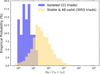 |
Fig. 3. Empirical probability distributions of |δω / (γ2 + γ3)| for the 21 identified (stable and AE -valid) isolated mode triads (blue and dotted) and their AE -valid and stable counterparts (yellow) that do not fulfill the isolation criterion. We choose the bin width in a similar way to what is done in Hogg (2008). |
Arras et al. (2003) have a different implicit ‘isolation criterion’: they stated that if the resonance is sharp, it is plausible that only the parent and two daughter modes are relevant for the mode amplitude dynamics. For sharp resonances, one expects |δω / (γ2+γ3)| to be small. Figure 3 shows the empirical probability distribution of |δω / (γ2+γ3)| for the 21 identified (stable, AE-valid) isolated mode triads, and their AE-valid and stable counterparts that do not fulfill the isolation criterion. While it is certainly true that |δω / (γ2+γ3)| is small for the isolated mode triads, there are non-isolated mode triads that have similarly low values of |δω / (γ2+γ3)|, which re-iterates the important role threshold surface luminosity fluctuations play in identifying such isolated mode triads.
Table 3 gives an overview of how restrictive the individual criteria are, and shows the effect of solely enforcing the validity or stability criteria. Many stable mode triads are identified, and fixed point stability is essentially defined by the hyperbolicity check. Both validity criteria are more restrictive than the stability criteria. It does not seem obvious for a g mode to participate in an isolated mode coupling scenario, as is reflected by the small number of identified isolated mode triads in Table 3. Moreover, strict enforcement of the TAR validity frequency hierarchies listed in for example Dhouib et al. (2021a) would further reduce the number of mode triads considered for asteroseismic modeling. This would however restrict the quadratic mode couplings identified for the 4 M⊙ near-ZAMS models from being used, contradicting observational evidence (e.g., V21). We therefore do not strictly enforce these frequency hierarchies.
4.3.2. Radial coupling contributions
For isolated mode triads that fulfill the stability and validity conditions, we compute a radial profile of the coupling coefficient η1(r) by integrating the overlap integrals in Eq. (22) up to an internal radial coordinate r instead of the stellar model surface radius R (i.e., r ≤ R and η1 ≡ η1(R)). The profile η1(r) then indicates the zones in the stellar interior for which contributions to the coupling coefficient are significant for these mode triads.
In the near-core regions the squared Brunt-Väisälä frequency (N2) profile has a (local) maximum due to the presence of a μ-gradient left behind by the receding convective core during the main sequence. This maximum introduces a sharp transition in N2 which changes the eigenfunctions: their modal inertia becomes more confined to the near-core region (Miglio et al. 2008; Michielsen et al. 2021), at the location of the (local) maximum. This can be rationalized by the increasing confinement of modal inertia to the TAR-valid near-core mixing zone with model age. The width of that maximum depends on the evolutionary stage: more evolved SPB models have wider N2 maxima, and some modes become trapped in the near-core regions (Moravveji et al. 2016; Michielsen et al. 2021). For these more evolved models, the instability strip for (k, m)=(0, 2) parent g modes also moves towards higher radial orders, further confining modal inertia to the oscillatory near-core regions. Both these effects likely explain why the contributions to coupling coefficients are more concentrated in the near-core regions for more evolved models.
Examples of such radial coupling coefficient profiles are given in Figs. 4 and 5, which display the N2 profile along with the coupling coefficient profile η1(r). The profile in Fig. 4 describes the coupling contributions for the mode triad characterized by g mode radial orders (n1, n2, n3) = (−22, −15, −53) in the mid-MS ΔXc, 1 model in Table 4. The near-ZAMS example displayed in Fig. 5 describes the coupling contributions for the mode triad characterized by g mode radial orders (n1, n2, n3) = (−14, −10, −26) in the ΔXc, 2(a) model of Table 4. These figures confirm that contributions to the coupling coefficient of the mode coupling in the mid-MS model are typically more confined to the near-core region in comparison to those contributions in the near-ZAMS model.
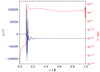 |
Fig. 4. Coupling coefficient and squared Brunt-Väisälä frequency (N2) profiles as a function of the fractional radius for the isolated mode triad with g mode radial orders (n1, n2, n3) = (−22, −15, −53) in the mid-MS ΔXc, 1 model of Table 4. |
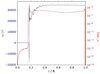 |
Fig. 5. Same as Fig. 4, but for the isolated mode triad with g mode radial orders (n1, n2, n3) = (−14, −26, −10) in the ΔXc, 2(a) model of Table 4. |
Linear co-rotating-frame frequencies Ωφ, largest absolute spin parameters |sφ| (of the triad modes), radial orders nφ and linear driving or linear damping rates γφ of g modes φ in all identified isolated (g) mode triads with ordering numbers (k1, k2, k3) = (0, 0, 0) and azimuthal orders (m1, m2, m3) = (2, 1, 1) for the models in Table 2 that yield stable and valid stationary solutions.
4.3.3. Properties of isolated g mode triads in SPB stars
Isolated mode triads can be identified for each model listed in Table 2. Their characteristic mode and triad properties are listed in Table 4, and their dimensionless model validity and stability estimators, including the order of magnitude of the coupling coefficient |η1|, are displayed in Table 5. It is clear from the largest absolute values of the spin parameters that at least one of the modes in the identified isolated mode triads is sub-inertial (i.e., |sφ|> 1), requiring the non-perturbative (TAR) description of the Coriolis force.
Dimensionless quantities for the mode triads listed in Table 4: dimensionless AE validity parameter ΨAE, absolute detuning-damping ratio |q| and absolute detuning-driving ratio |q1|, the driving-damping rate ratios ϑ2 and ϑ3, as well as the order of magnitude of the energy-normalized coupling coefficient, 𝒪|η1|.
The Doppler shift causes a logical trend to appear when correlating the average values of Ωφ with a change in the rotation frequency (i.e., upon comparison of mode frequencies for the models ΔXc, 2(a) and ΔXc, 2(b)): Ωφ decreases for increasing rotation rates. This trend is only weakly influenced by the effect of the Coriolis force for these sectoral prograde g or equatorial Kelvin waves, which is not the case for non-sectoral modes (due to geostrophic balance; see e.g., Gill 1982; Townsend 2005; Daszyńska-Daszkiewicz et al. 2015; Szewczuk & Daszyńska-Daszkiewicz 2017).
The co-rotating-frame mode frequencies also (on average) decrease for higher-mass models, and decrease with model age. This change with mass can be attributed to the more massive SPB models having a larger model radius, which enlarges the pulsation cavity, although it is to a degree counteracted by the decrease in Ω.
Mode frequency in the co-rotating frame is instrumental for determining linear, heat-driven mode excitation: it determines the geometrically optimal driving region for a mode, which needs to coincide with the Z bump for the mode to be linearly excited in an SPB star. In general, higher radial order g modes3 – which have lower frequencies and are therefore more susceptible to rotational effects – are excited in more evolved models (on the main sequence). The expected higher mode densities for more evolved stars might explain why only one isolated mode triad was identified for the fiducial model. The linear (vibrational) stability sensitively depends on the opacity profile of any particular stellar model (e.g., Daszyńska-Daszkiewicz et al. 2017). A change in opacity profile can therefore lead to the identification of different isolated mode triads.
Stabilization of the (k, m)=(0, 1) g modes in more rapidly rotating stars (e.g., Townsend 2005) can lead to opportunities for non-linear excitation by a parametric resonance, as it enlarges the pool of potential daughter modes with which combination can be made. A physical explanation of the effect of rotation within the TAR on mode excitation by the κ mechanism can be found in Ushomirsky & Bildsten (1998) and Townsend (2005). That increasing potential for mode combination with larger rotation rate can be observed in the ‘Total’ column of Table 3, where more combinations are considered for the more rapidly rotating model ΔXc, 2(b), if compared to the number of combinations considered for model ΔXc, 2(a). The stabilizing effect for the parent (k, m)=(0, 2) g modes comparatively seems weaker (as was also observed by Townsend 2005): only one of the parent modes is stabilized, in comparison to seven of the daughter modes, when we compare the ΔXc, 2(a) and ΔXc, 2(b) models. In this case, we identify four isolated triads for model ΔXc, 2(b), and two isolated triads for the slower-rotating model ΔXc, 2(a). However, the stabilizing effect does not necessarily mean that we can identify more isolated mode triads for rapid rotators, because those triads need to fulfill the stability and validity criteria.
The range of |q1| for the identified isolated mode triads is [104, 100] (using the notation of Table 2). This indicates that the two rightmost panels on the top of Fig. 2, as well as the panels on the bottom row of Fig. 2, describe the linear stability of the isolated stationary solutions. These solutions’ resonant nature is important, as is indicated by the values of |q| being of the order of unity to ten, affecting the stationary amplitude (48).
We can identify only one isolated harmonic resonant triad (for the ΔXc, 1 model), which is a small number in comparison to the 20 identified resonances of the combination type Ω1 ≈ Ω2 + Ω3. It therefore seems comparatively harder to satisfy all stability and validity conditions for harmonic resonances, which provides a reason for why only a few of such resonances are identified in the observational data of V21.
We only consider combinations of a small number of modes in this proof-of-concept study and do not study the dependence of non-linear parameters – such as the coupling coefficient – on stellar parameters in detail.
5. Impact on asteroseismic modeling
In this section, we discuss how the non-linear theoretically predicted observables defined in Sect. 3 can aid or complement current frequency-based asteroseismic modeling of SPB stars. The various non-linear observables of interest, or derived quantities thereof, are listed in Table 6.


5.1. Oscillation frequency and combination phase observables
We find that the non-linear frequency shifts of the isolated mode triads are small in comparison to the (linear) inertial mode frequencies, as is illustrated by the values in the column displaying values of  in Table 6, which shows the largest value of the frequency shift for any of the three modes in the isolated triad, expressed in units of the inertial mode frequency. These dimensionless frequency shifts are typically of order 10−3 to 10−4, and we find no clear correlations with any of the model parameters (potentially due to the small number of modes considered).
Translated to units of d−1, this means that there are several frequencies whose (non-linear) frequency shifts are of order 10−5 d−1 or smaller, rendering them of similar order as the typical errors for the frequencies derived from 4-year Kepler light curves (e.g., Bowman & Michielsen 2021). The largest shifts are obtained for the modes in the faster-rotating models, and are of order 10−2 or 10−3 d−1, which is approximately two orders of magnitude larger than typical uncertainties. In practice, the resonant non-linear frequency shifts are hard to distill from frequency lists deduced from prewhitening analyses similar to what was done in V21. The non-resonant frequency shifts are even smaller, justifying the approximation of using linear frequencies in asteroseismic modeling.
We show the zero-point-corrected non-linear combination phases  for all identified isolated mode triads in Table 6, where
  . We find no specific trends for these combination phases when correlated with other model parameters (potentially due to the small number of modes considered). In principle, such phases can be compared with observed relative phases, if the relative phase at the zero point is accounted for. The latter is however dependent on the initial values of the individual mode phases, ϕ0, which are unconstrained.
5.2. Amplitude ratio observables
The stationary surface luminosity fluctuation ratios  and
and  offer the best constraints for asteroseismic modeling. We find that most of these ratios are smaller than unity, indicating that most of the stationary-state (or saturation) energies of the linearly driven (k, m)=(0, 2) parent modes are larger than those of the (k, m)=(0, 1) daughter modes that are linearly damped and parametrically excited. Daughter modes have larger stationary mode amplitude ratios
  only for certain mode triads in the 4 M⊙ near-ZAMS models ΔXc, 2(a) and ΔXc, 2(b), as well as the 6 M⊙ near-TAMS models ΔMini, 1. For these specific mode triads, the other daughter mode’s amplitude is significantly smaller than that of the parent mode.
The stationary amplitude ratios (76) depend on the ratios of the mode quality factors that express the number of periods necessary to linearly increase or decrease modal energy by a factor of e. Such ratios are inversely proportional to ϑ2 or ϑ3 and proportional to the frequency ratio Ω2 / Ω1 or Ω3 / Ω1. We find that the frequency ratios for these specific isolated mode triads that have larger-amplitude daughter modes are not particularly different from those in other identified isolated mode triads, as can be rationalized from the co-rotating mode frequency values in Table 4. The observed difference in amplitude ratio is thus is mostly due to different values of ϑ2. The smaller ϑ2, the longer the linear damping timescale of daughter mode 2 is, in comparison to the linear driving timescale of parent mode 1. Based on the listed values of ϑ2 in Table 5, this effect seems to become important when ϑ2 ≲ 0.13 ≡ ϑ2, b, that is, when the linear damping rate of one of the daughter modes is less than 13% of the linear driving rate of the parent mode. We also estimate the value of ϑ2 at which this effect becomes important by performing a linear regression between the ϑ2 and  values of four isolated mode triads in Table 5. Specifically, we construct a regression model using the ϑ2 and
  values obtained from the two mode triads with parent-daughter amplitude ratios greater than unity but approaching the unity limit the closest, and the values of these quantities obtained from those mode triads with parent-daughter amplitude ratios smaller than unity that approach the unity limit the closest. The linear regression yields a linear slope of −0.08 ± 0.04 (ϑ2 per unit of
  ) and an intercept 0.22 ± 0.06, when we assume normally distributed residuals. This leads to an estimated boundary
  that is consistent with the earlier defined boundary ϑ2, b.
In general, energy transfer occurs from the parent to the daughter mode only if the latter’s energy is smaller than the former’s (e.g., Arras et al. 2003). However, if one of the daughter modes participating in the mode triad is strongly damped (linearly), mode β, when the other daughter mode, mode α, is only weakly damped (linearly), we find that daughter mode α can saturate at larger energies than the parent mode. In such situations the parent mode needs to transfer a lot of energy to the daughter modes per cycle in order to overcome the strong linear damping of daughter mode β and reach a stationary state.
Isolated parametric couplings in which both daughter modes attain amplitudes larger than the parent mode are not observed in our calculations. Of the 276 835 potential triads considered in this work, only 32 non-AE valid triads have both daughter-parent luminosity fluctuation energy ratios (76) greater than unity, which all originate from the ΔMini, 1 model. Of those 32 solutions, 26 satisfy q > Q1, the necessary but not sufficient condition for both stationary daughter-parent rotating-frame mode energy ratios (52) to be greater than unity, because of Eqs. (49) and (78). The other 6 solutions are relatively close to satisfying that criterion (q and Q1 are of the same order of magnitude) and likely obtain daughter-parent mode luminosity fluctuation energy ratios (76) greater than unity because of the differing ratios of amplitude conversion factors oA, φ. Given the typical values of Ωφ, γφ and q listed in Tables 4 and 5, as well as the quality factor ranges listed in Table 2, we deem it unlikely to encounter isolated solutions of this kind.
5.3. Comparison with observations of SPB stars
To assess the impact of mode amplitude ratios on period spacing pattern modeling, we compare daughter-parent surface luminosity fluctuation ratios predicted by our formalism with observed equivalents derived for the ensemble of 38 SPB stars of V21. We limit ourselves to comparison among theoretically predicted amplitude ratios and observed equivalents of sum frequencies, because these make up the majority of the isolated mode triads listed in Table 5. Our comparison is also valid for difference frequencies, because the AEs and stationary solutions for these difference frequencies are of the same form as those of sum frequencies (see Appendix F).
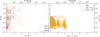 |
Fig. 6. Observed daughter-parent amplitude ratios |


V21 generated variability models for the light curves, hereafter referred to as (harmonic) light curve models, of 38 SPB stars using five different harmonic analysis strategies. In this work, we use the models generated by their strategy 3, which uses the signal-to-noise ratios to determine the significance of detected variability signals, because this resembles commonly used strategies in literature (see Table 1 and the corresponding discussion in Sect. 2.2 of V21 for additional details). They assigned pseudo-classes to the different members of the ensemble of analyzed SPB stars to denote the difficulties encountered during the analysis process: high-fsv stars had light curves that were described adequately by the harmonic light curve models; high mode density stars had many close-spaced frequencies in their Fourier transforms or Lomb-Scargle periodograms; and outbursting stars were found to have distinct variability ‘outbursts’ in their light curves, resulting in many close-spaced and high-amplitude frequency groups (see V21). To select the relevant observed signals for our comparison, we look for sum-frequency resonance combinations of three signals that are part of the light curve models and fulfill the resonance criterion |ν1 − ν2 − ν3|≤ℜν + σν, prop (with σν, prop the propagated uncertainty of the observed frequency difference ν1 − ν2 − ν3 and ν1, ν2 and ν3 the observed frequencies). These combinations also need to contain (i) at least one of the two highest-amplitude signals in the light curve model, and (ii) lower-amplitude components (i.e., not one of the two highest-amplitude signals) that are not present in other considered combinations. The low-over-highest frequency amplitude ratios of these combinations,  (i.e., two ratios per combination), are displayed in the left panel of Fig. 6 as a function of the minimal frequency νmin of the three modes in the combination, as measured within the inertial reference frame. Under the assumption that the non-linear parametric resonant coupling process dominates the energy transfer among the considered modes, we hereafter refer to
  as the observed daughter-parent amplitude ratios; under that assumption, νmin is the minimal daughter mode frequency. Because the stationary combination phase observable
  defined in Eq. (82) depends on the unconstrained initial zero points of the individual mode phases and because no trends are observed in the zero-point-corrected non-linear combination phases
  of isolated mode triads listed in Table 6, we do not enforce conditions on the relative phase of these observed combinations of signals, unlike V21.
One compares the observed daughter-parent amplitude ratios with the relevant computed daughter-parent (stationary) surface luminosity fluctuation ratios |𝔏d| / |𝔏p| of triads found among the (k, m)=(0, 1) daughter g modes and of the (k, m)=(0, 2) parent g modes computed by GYRE for the models listed in Table 2 (shown in the right panel of Fig. 6). These mode triads have small frequency detunings (34) and satisfy all stability criteria, and we further distinguish between triads with modes that satisfy (i) only the stability criteria, or (ii) the stability criteria and the AE validity criterion, or (iii) all stability and validity criteria (i.e., these are the isolated mode triads). The minimal mode frequency observable  (used as the x-axis variable in the right panel of Fig. 6) is smaller than the non-linear frequency shift (54) for some of the considered modes in mode triads with linearly stable solutions (i.e., triads with modes that only satisfy the stability criteria and none of the validity criteria). In that case, we compute their alias frequencies in the frequency range [24.4512, 0] d−1 (using the notation in Table 2; i.e., up to the notional Kepler long-cadence Nyquist frequency; Chaplin et al. 2014). Such aliased signals would however have their amplitude ratios affected by their splitting, which we do not account for in this work. The predicted surface luminosity fluctuation ratios of these alias frequencies are therefore shown on the right panel of Fig. 6 as faint (orange-red) symbols.
The ensemble of stationary surface luminosity fluctuation ratios of computed triads seems to be able to explain the low-amplitude-ratio part of the ensemble of observed daughter-parent amplitude ratios, as can be derived from the panels in Fig. 6. Some SPB modeling targets, for example KIC008714886, show promise for matching a part of their observed amplitude ratios with their theoretically predicted equivalent. Other targets (notably the slow rotator KIC0010526994) have observed daughter-parent amplitude ratios that are all much greater than unity, which we do not have in the calculated ratios.
The absence of high theoretically predicted surface luminosity fluctuation ratios (52) might be caused by our choice of opacity tables, because they determine the linear growth or linear damping rates of the modes. For example, one of the analyzed SPB stars, KIC0010536147, is on the massive end of the SPB instability region (according to the stellar parameters determined in Pedersen 2022), where, according to our simulations that account for the classical κ mechanism driving mechanism, no (k, m)=(0, 2) parent modes are excited (see Table 2). The required changes in opacity to reach the highest observed amplitude ratios are, however, unlikely to be realistic. The modified opacities of Daszyńska-Daszkiewicz et al. (2017) used in modeling the linear stability of the hybrid main-sequence early B-type pulsator ν Eridani for example lead to normalized driving rates that were only two to four times larger than the unmodified driving rates. Asteroseismic modeling of dedicated targets is needed to further assess the effect of opacity on theoretical surface luminosity fluctuation ratios.
Additionally, some of the observed modes might have different nonradial geometries (i.e., different values of m, k) than the ones considered in the limited number of simulations carried out for this work. For example, the period spacing patterns considered by Pedersen et al. (2021) are made up of zonal (k, m)=(1, 0) dipole g modes for 9 of their considered 26 SPB stars, and one star, KIC008714886, has an identified retrograde (k, m)=(0, −1) dipole g mode period spacing pattern (see Supplementary Table 1 of Pedersen et al. 2021). When couplings between g modes other than the ones considered in this work have linear driving or linear damping rates, frequencies, as well as amplitude conversion factors oA, φ of the same order as those obtained for the g modes considered in this work, we expect to obtain similar theoretically predicted luminosity fluctuation ratios. We note, however, that for such different combinations the parent mode can be a lower frequency mode. An example of such a combination that satisfies the coupling coefficient selection rules is the triad that consists of a driven (k, m)=(0, 1) parent mode α, a damped (k, m)=(0, 2) daughter mode β, and a damped (k, m)=(0, −1) daughter mode γ. The damped (k, m)=(0, 2) daughter mode β can have a lower frequency than the parent mode α in the co-rotating frame, while having a higher frequency in the inertial frame. Such a damped (k, m)=(0, 2) mode β would therefore be labeled as the parent when following the rules used to generate the observed daughter-parent amplitude ratios shown in Fig. 6. For comparison with the theoretically predicted daughter-parent surface luminosity fluctuation ratios, the relevant observed amplitude ratios then need to either be computed (as the ratio of the current amplitude ratios) or inverted. In our example, we need to compute the amplitude ratio of modes β and γ  ), and we need to invert the currently computed amplitude ratio of modes α and β.
We also deem it likely that some of the high observed amplitude ratios can be attributed to other amplitude saturation mechanisms, such as multi-mode coupling or higher-order couplings. Correlation of the mean values of the 10 largest mode amplitudes (determined from the light curve models) with the mean values of the 10 largest identified amplitude ratios for each of the different SPB stars considered by V21 for example yields a positive Spearman correlation coefficient. This suggests that higher-order couplings might be needed to explain the high amplitude ratios of high-amplitude SPB pulsators.
6. Conclusions
We derive a theoretical oscillation modeling framework that describes non-linear three-mode coupling among gravito-inertial (g) modes of Slowly Pulsating B (SPB) stars within the Traditional Approximation for Rotation (TAR; e.g., Longuet-Higgins 1968; Lee & Saio 1997; Townsend 2003; Mathis 2013), extending and correcting terms in the formalism of L12 (see Appendix C). This framework relates the g mode adiabatic eigenfunctions to potential non-linear energy exchange between the modes, by computing three-mode (energy-scaled) coupling coefficients |η1| based on a phase space mode decomposition inserted in the relevant coupled equations of motion. To describe three-mode resonant couplings, we derive amplitude equations (AEs) from the coupled equations of motion for a sum-frequency resonance Ω1 ≃ Ω2 + Ω3, using the multiple time scales perturbation method (e.g., Nayfeh 1973, 1981; Nayfeh & Mook 1979). These coupling coefficients need to satisfy angular selection rules (24) and (25) if energy is to be exchanged among the modes. The isolated stable stationary solutions of these AEs (i.e., their stable fixed points) then describe locked three-mode resonant couplings among g modes in rapidly rotating g-mode pulsating stars, such as SPB stars.
We use this framework to compute examples of isolated mode couplings in stellar structure and pulsation models that represent SPB stars analyzed in V21. We limit ourselves to computing couplings among g modes with ordering numbers (k1, k2, k3) = (0, 0, 0) and azimuthal orders (m1, m2, m3) = (2, 1, 1); the most frequently observed modes in SPB stars (see e.g., Pedersen et al. 2021; Szewczuk et al. 2021; Pedersen 2022). The locked mode solutions have to fulfill multiple stability and validity criteria to describe physical three-mode coupling scenarios in such stars. To ensure stability of the three-mode stationary solution, it needs to be hyperbolic, the resonance must be parametric, and the solution must fulfill the condition in Eq. (61a) and the linear quartic stability criterion (64). The validity of the solution is guaranteed if it fulfills the AE validity condition ΨAE ≤ 0.1 (with ΨAE defined in Eq. (83)), and the isolation criterion. The most restricting of all these conditions is the isolation criterion, which ensures that no multi-mode coupling scenarios take place. We find that the restriction to sharp resonances as done by Arras et al. (2003) overestimates the number of isolated mode triads.
By performing coupling computations up to a certain inner radius, we map the regions that contribute significantly to the mode coupling. Typically, we obtain strong contributions to the resonant coupling among the three g modes in the near-core zones of the SPB models, where N2 peaks and modes can become (partially) trapped (Miglio et al. 2008; Michielsen et al. 2021). For more evolved models, this N2 maximum is wider and the κ mechanism typically excites higher radial order modes, which are increasingly confined to the near-core zones. Conversely, for less evolved models, significant contributions to |η1| can be found outside of the near-core zones.
Linear heat-driven vibrational instability defines which modes are available for the non-linear (parametric) couplings we study in this work. The individual mode frequencies depend on a variety of factors, including rotation rate, evolutionary stage, and mass, among others. These frequencies are important, because they define the optimal linear driving regions of the corresponding modes. The linear driving of g modes in SPB stars, however, is ultimately reliant upon the opacity profiles inside the Fe bump. Opacity tables used during stellar modeling define the opacity gradients in the driving zones, and therefore influence (i) the number of possible mode triads that can be formed for a specific model, but also (ii) the linear driving and linear damping rates themselves. These linear driving and linear damping rates affect the non-linear observables, such as the computed stationary mode luminosity fluctuations and their ratios.
For the few models considered in this work, we find no obvious correlations for changes in the coupling coefficients (22) with changes in model parameters. It is not clear whether such trends can be detected if the number of models and the number of considered modes is increased while varying model parameters such as the opacity tables. Because the absolute values of the detuning-damping ratio, |q|, are larger than unity, it is clear however that the resonant nature of the coupling strongly determines the stationary state mode amplitudes (48).
The non-linear frequency shifts (54) for isolated triads are small enough to neglect when compared with the typical errors for the frequencies derived from 4-year Kepler light curves, and the combination phases (82) contain an unconstrained initial mode phase parameter. The best constraints for asteroseismic modeling are therefore obtained from the predicted luminosity fluctuation ratios (76) of coupled modes. Most of these ratios indicate that the (k, m) = (0, 2) parent g modes considered in this work have higher apparent mode amplitudes than their coupled (k, m) = (0, 1) daughter g modes. We obtain disparate linear daughter mode damping rates for each of the isolated mode triads. If one of the linearly damped daughter modes in the isolated mode triad is weakly damped (linearly; at a rate ≲13% that of the parent linear driving rate), we find that that daughter mode can saturate at a higher amplitude than its coupled parent mode. We deem it unlikely that isolated solutions exist in which both daughter-parent amplitude ratios are greater than unity, because of the typical values for the quality factors and detuning-damping ratios associated with g modes in SPB star models.
The monochromatic stationary luminosity fluctuation ratios are consistent with some of the lowest amplitude ratios  observed in the Kepler space photometric time series of some of the target SPB stars (see Sect. 5.3). Even the lowest order model of resonant non-linear mode coupling developed in this work can thus aid future asteroseismic modeling of rapidly rotating SPB stars based on g modes, because it offers additional constraints on some of the observed combination frequencies based on stationary amplitude ratios of specific, resonantly coupled modes. This can in principle also serve as an additional source of mode identification. The logical next step in understanding non-linear amplitude saturation is to apply this framework to the modeling of some of the SPB stars analyzed in V21 by integrating our monochromatic predictions over the Kepler passband.
It should be investigated whether larger resonantly coupled networks of modes or higher-order and r − g mode coupling can saturate some of the unexplained observed candidate couplings in SPB stars. Higher-order coupling will definitely already include self-saturation effects that are neglected in the current formalism (see e.g., Van Hoolst et al. 1998 for an example of a study that included these effects for radial modes while neglecting rotation, and Gastine & Dintrans 2008a,b for direct numerical simulations of the κ mechanism and non-linear saturation for radial modes in Cepheids). Mode triads containing g modes not considered in this work can also explain the presence of some of the highest observed amplitude ratios obtained in this work.
Other authors, such as Lee (2001) and Aprilia & Saio (2011), used a mode expansion formalism that did not invoke the TAR and accounted for linear mode couplings to describe the linear eigenmodes. They found that their formalism linearly stabilizes some of the g modes that were excited when the TAR was assumed (i.e., constituting a systematical error). That method, which truncates the series expansion at some manageable expansion order, is computationally more intensive, and might not be accurate (Dziembowski et al. 2007). Perhaps the hybrid expansion method discussed in Chapter 7 of Goupil et al. (2013) that describes linear mode coupling using expansions of modes whose angular eigenfunctions are described by Hough functions is a good compromise that softens the computational load with increasing expansion order, compared to the original expansion formalism. Because we find that the non-linear saturation is crucially dependent on the linear excitation properties, in-depth investigations of the linear vibrational instability of g modes in SPB stars using the latest improvements in opacity computations are crucial for future non-linear excitation studies (e.g., Daszyńska-Daszkiewicz et al. 2017). Such investigations will allow us to estimate the systematical error we make in the theoretical predictions of surface luminosity fluctuation ratios due to opacity.
The strength of the Coriolis force is determined by the Coriolis frequency 2Ω. The TAR frequency hierarchies 2|Ω|≪|N| and |Ωφ|≪|N|, where Ωφ is the real-valued frequency of pulsation mode φ in the co-rotating reference frame, impose strong stratification in specific regions of the stellar interior, through which the low-frequency waves described within the TAR propagate (see e.g., Dhouib et al. 2021a).
Such periodic frequency and/or amplitude modulation (or even irregular behavior) can be simulated (numerically) using the amplitude equations or coupled-mode equations derived in this work.
A g mode α is considered to have a higher radial order than g mode β when nα < nβ (i.e., when the absolute value of its radial order is larger).
The repository can directly be accessed using the following link: https://doi.org/10.5281/zenodo.10814654.
Acknowledgments
The research leading to these results received funding from the KU Leuven Research Council (grant C16/18/005: PARADISE, with PIs CA and TVH). The research leading to part of these results has also received funding from the European Research Council (ERC) under the Horizon Europe programme (Synergy Grant agreement N°101071505: 4D-STAR). Funded by the European Union. Views and opinions expressed are however those of the author(s) only and do not necessarily reflect those of the European Union or the European Research Council. Neither the European Union nor the granting authority can be held responsible for them. JVB and CA acknowledge support from the Research Foundation Flanders (FWO) under grant agreements N°V421221N (Travel Grant) and N°K802922N (Sabbatical leave). This research was also supported in part by the National Science Foundation under Grant No. PHY-1748958. JVB is grateful to Dominic Bowman for the useful discussion and comments on the manuscript. JVB is also grateful to Michel Rieutord, Rony Keppens and Timothy Van Reeth for the useful comments on his PhD manuscript, which improved this work. CA is grateful for the kind hospitality offered by the staff of the Center for Computational Astrophysics at the Flatiron Institute of the Simons Foundation in New York during her work visits in the fall of 2022 and spring of 2023. Throughout this work we have made use of the following Python packages: LMFIT (Newville et al. 2020), SCIPY (Virtanen et al. 2020), NUMPY (Harris et al. 2020), PANDAS (McKinney et al. 2010), and MATPLOTLIB (Hunter 2007). We thank their authors for making these great software packages open source.
References
- Aerts, C. 2021, Rev. Mod. Phys., 93, 015001 [Google Scholar]
- Aerts, C., & Tkachenko, A. 2023, arXiv e-prints [arXiv: 2311.08453] [Google Scholar]
- Aerts, C., de Pauw, M., & Waelkens, C. 1992, A&A, 266, 294 [NASA ADS] [Google Scholar]
- Aerts, C., Christensen-Dalsgaard, J., & Kurtz, D. W. 2010, Asteroseismology (Springer) [Google Scholar]
- Aerts, C., Molenberghs, G., Michielsen, M., et al. 2018, ApJS, 237, 15 [Google Scholar]
- Aikawa, T. 1984, MNRAS, 206, 833 [NASA ADS] [CrossRef] [Google Scholar]
- Aprilia, L. U., & Saio, H. 2011, MNRAS, 412, 2265 [NASA ADS] [CrossRef] [Google Scholar]
- Arras, P., Flanagan, E. E., Morsink, S. M., et al. 2003, ApJ, 591, 1129 [NASA ADS] [CrossRef] [Google Scholar]
- Bernstein, D. S. 2009, Matrix Mathematics: Theory, Facts, and Formulas, Second Edition (Princeton: Princeton University Press) [CrossRef] [Google Scholar]
- Betounes, D. 2010, Differential Equations: Theory and Applications (New York: Springer-Verlag) [CrossRef] [Google Scholar]
- Bhatia, R. 2007, Positive Definite Matrices (Princeton: Princeton University Press) [Google Scholar]
- Björklund, R., Sundqvist, J. O., Puls, J., & Najarro, F. 2021, A&A, 648, A36 [EDP Sciences] [Google Scholar]
- Bowman, D. M., & Michielsen, M. 2021, A&A, 656, A158 [NASA ADS] [CrossRef] [EDP Sciences] [Google Scholar]
- Bowman, D. M., Kurtz, D. W., Breger, M., Murphy, S. J., & Holdsworth, D. L. 2016, MNRAS, 460, 1970 [NASA ADS] [CrossRef] [Google Scholar]
- Buchler, J. R. 1993, Ap&SS, 210, 9 [NASA ADS] [CrossRef] [Google Scholar]
- Buchler, J. R., & Goupil, M. J. 1984, ApJ, 279, 394 [CrossRef] [Google Scholar]
- Buchler, J. R., & Regev, O. 1983, A&A, 123, 331 [NASA ADS] [Google Scholar]
- Buchler, J. R., Goupil, M. J., & Serre, T. 1995, A&A, 296, 405 [NASA ADS] [Google Scholar]
- Buchler, J. R., Goupil, M. J., & Hansen, C. J. 1997, A&A, 321, 159 [NASA ADS] [Google Scholar]
- Burkart, J., Quataert, E., Arras, P., & Weinberg, N. N. 2012, MNRAS, 421, 983 [NASA ADS] [CrossRef] [Google Scholar]
- Burkart, J., Quataert, E., Arras, P., & Weinberg, N. N. 2013, MNRAS, 433, 332 [NASA ADS] [CrossRef] [Google Scholar]
- Burkart, J., Quataert, E., & Arras, P. 2014, MNRAS, 443, 2957 [NASA ADS] [CrossRef] [Google Scholar]
- Cesari, L. 1971, Asymptotic Behavior and Stability Problems in Ordinary Differential Equations (Berlin, Heidelberg: Springer), 1 [Google Scholar]
- Chaplin, W. J., Elsworth, Y., Davies, G. R., et al. 2014, MNRAS, 445, 946 [NASA ADS] [CrossRef] [Google Scholar]
- Cowling, T. G. 1941, MNRAS, 101, 367 [NASA ADS] [Google Scholar]
- Cox, J. P., & Giuli, R. T. 1968, Principles of Stellar Structure (New York: Gordon and Breach) [Google Scholar]
- Dappen, W., & Perdang, J. 1985, A&A, 151, 174 [NASA ADS] [Google Scholar]
- Daszyńska-Daszkiewicz, J., Dziembowski, W. A., Jerzykiewicz, M., & Handler, G. 2015, MNRAS, 446, 1438 [CrossRef] [Google Scholar]
- Daszyńska-Daszkiewicz, J., Pamyatnykh, A. A., Walczak, P., et al. 2017, MNRAS, 466, 2284 [CrossRef] [Google Scholar]
- De Cat, P., & Aerts, C. 2002, A&A, 393, 965 [NASA ADS] [CrossRef] [EDP Sciences] [Google Scholar]
- Degroote, P., Briquet, M., Catala, C., et al. 2009, A&A, 506, 111 [NASA ADS] [CrossRef] [EDP Sciences] [Google Scholar]
- Degroote, P., Aerts, C., Baglin, A., et al. 2010, Nature, 464, 259 [Google Scholar]
- Dhouib, H., Prat, V., Van Reeth, T., & Mathis, S. 2021a, A&A, 652, A154 [NASA ADS] [CrossRef] [EDP Sciences] [Google Scholar]
- Dhouib, H., Prat, V., Van Reeth, T., & Mathis, S. 2021b, A&A, 656, A122 [NASA ADS] [CrossRef] [EDP Sciences] [Google Scholar]
- Dziembowski, W. 1982, Acta Astron., 32, 147 [NASA ADS] [Google Scholar]
- Dziembowski, W. A. 1993, ASP Conf. Ser., 40, 521 [NASA ADS] [Google Scholar]
- Dziembowski, W., & Krolikowska, M. 1985, Acta Astron., 35, 5 [NASA ADS] [Google Scholar]
- Dziembowski, W., Krolikowska, M., & Kosovichev, A. 1988, Acta Astron., 38, 61 [NASA ADS] [Google Scholar]
- Dziembowski, W. A., Moskalik, P., & Pamyatnykh, A. A. 1993, MNRAS, 265, 588 [NASA ADS] [Google Scholar]
- Dziembowski, W. A., Daszyńska-Daszkiewicz, J., & Pamyatnykh, A. A. 2007, MNRAS, 374, 248 [NASA ADS] [CrossRef] [Google Scholar]
- Essick, R., & Weinberg, N. N. 2016, ApJ, 816, 18 [Google Scholar]
- Frieman, E., & Rotenberg, M. 1960, Rev. Mod. Phys., 32, 898 [Google Scholar]
- Friedman, J. L., & Schutz, B. F. 1978a, ApJ, 221, 937 [NASA ADS] [CrossRef] [Google Scholar]
- Friedman, J. L., & Schutz, B. F. 1978b, ApJ, 222, 281 [NASA ADS] [CrossRef] [Google Scholar]
- Fuller, J. 2017, MNRAS, 472, 1538 [Google Scholar]
- Fuller, J., & Lai, D. 2012, MNRAS, 420, 3126 [NASA ADS] [CrossRef] [Google Scholar]
- Fuller, J., Derekas, A., Borkovits, T., et al. 2013, MNRAS, 429, 2425 [CrossRef] [Google Scholar]
- Fuller, J., Luan, J., & Quataert, E. 2016, MNRAS, 458, 3867 [Google Scholar]
- Gaia Collaboration (Prusti, T., et al.) 2016, A&A, 595, A1 [NASA ADS] [CrossRef] [EDP Sciences] [Google Scholar]
- Gastine, T., & Dintrans, B. 2008a, A&A, 484, 29 [NASA ADS] [CrossRef] [EDP Sciences] [Google Scholar]
- Gastine, T., & Dintrans, B. 2008b, A&A, 490, 743 [NASA ADS] [CrossRef] [EDP Sciences] [Google Scholar]
- Gautschy, A., & Saio, H. 1993, MNRAS, 262, 213 [NASA ADS] [CrossRef] [Google Scholar]
- Gill, A. 1982, Atmosphere-Ocean Dynamics (New York: Academic Press) [Google Scholar]
- Goldstein, J., & Townsend, R. H. D. 2020, ApJ, 899, 116 [NASA ADS] [CrossRef] [Google Scholar]
- Goupil, M.-J., & Buchler, J. R. 1994, A&A, 291, 481 [NASA ADS] [Google Scholar]
- Goupil, M. J., Dziembowski, W. A., & Fontaine, G. 1998, Baltic Astron., 7, 21 [NASA ADS] [Google Scholar]
- Goupil, M., Belkacem, K., Neiner, C., Lignières, F., & Green, J. J. 2013, Studying Stellar Rotation and Convection: Theoretical Background and Seismic Diagnostics, 865 [CrossRef] [Google Scholar]
- Guckenheimer, J., & Holmes, P. 1983, Nonlinear Oscillations, Dynamical Systems, and Bifurcations of Vector Fields (New York, NY: Springer) [CrossRef] [Google Scholar]
- Guo, Z. 2020, ApJ, 896, 161 [NASA ADS] [CrossRef] [Google Scholar]
- Guo, Z. 2021, Front. Astron. Space Sci., 8, 67 [NASA ADS] [Google Scholar]
- Hahn, W. 1967, Stability of Motion., Die Grundlehren der mathematischen Wissenschaften, in Einzeldarstellungen mit besonderer Berücksichtigung der Anwendungsgebiete: 138 (Berlin Heidelberg: Springer) [Google Scholar]
- Harris, C. R., Millman, K. J., van der Walt, S. J., et al. 2020, Nature, 585, 357 [NASA ADS] [CrossRef] [Google Scholar]
- Henneco, J., Van Reeth, T., Prat, V., et al. 2021, A&A, 648, A97 [EDP Sciences] [Google Scholar]
- Hogg, D. W. 2008, arXiv e-prints [arXiv:0807.4820] [Google Scholar]
- Hunter, J. D. 2007, Comput. Sci. Eng., 9, 90 [NASA ADS] [CrossRef] [Google Scholar]
- Koch, D. G., Borucki, W. J., Basri, G., et al. 2010, ApJ, 713, L79 [Google Scholar]
- Kubicek, M., & Marek, M. 1983, Computational Methods in Bifurcation Theory and Dissipative Structures (Berlin, Heidelberg: Springer) [CrossRef] [Google Scholar]
- Kumar, P., & Goodman, J. 1996, ApJ, 466, 946 [NASA ADS] [CrossRef] [Google Scholar]
- Lai, D., & Wu, Y. 2006, Phys. Rev. D, 74, 024007 [NASA ADS] [CrossRef] [Google Scholar]
- Lee, U. 2001, ApJ, 557, 311 [NASA ADS] [CrossRef] [Google Scholar]
- Lee, U. 2012, MNRAS, 420, 2387 [NASA ADS] [CrossRef] [Google Scholar]
- Lee, U. 2022, MNRAS, 513, 2522 [NASA ADS] [CrossRef] [Google Scholar]
- Lee, U., & Saio, H. 1997, ApJ, 491, 839 [Google Scholar]
- Longuet-Higgins, M. S. 1968, Philos. Trans. R. Soc. London Ser. A, 262, 511 [NASA ADS] [CrossRef] [Google Scholar]
- Lynden-Bell, D., & Ostriker, J. P. 1967, MNRAS, 136, 293 [Google Scholar]
- Mathis, S. 2013, in Transport Processes in Stellar Interiors, eds. M. Goupil, K. Belkacem, C. Neiner, F. Lignières, & J. J. Green, 865, 23 [Google Scholar]
- Mathis, S., & Prat, V. 2019, A&A, 631, A26 [NASA ADS] [CrossRef] [EDP Sciences] [Google Scholar]
- McKinney, W. 2010, in Proceedings of the 9th Python in Science Conference, eds. S. van der Walt, & J. Millman, 56 [Google Scholar]
- Michielsen, M., Pedersen, M. G., Augustson, K. C., Mathis, S., & Aerts, C. 2019, A&A, 628, A76 [NASA ADS] [CrossRef] [EDP Sciences] [Google Scholar]
- Michielsen, M., Aerts, C., & Bowman, D. M. 2021, A&A, 650, A175 [NASA ADS] [CrossRef] [EDP Sciences] [Google Scholar]
- Miglio, A., Montalbán, J., Noels, A., & Eggenberger, P. 2008, MNRAS, 386, 1487 [Google Scholar]
- Moravveji, E., Aerts, C., Pápics, P. I., Triana, S. A., & Vandoren, B. 2015, A&A, 580, A27 [NASA ADS] [CrossRef] [EDP Sciences] [Google Scholar]
- Moravveji, E., Townsend, R. H. D., Aerts, C., & Mathis, S. 2016, ApJ, 823, 130 [NASA ADS] [CrossRef] [Google Scholar]
- Morsink, S. M. 2002, ApJ, 571, 435 [NASA ADS] [CrossRef] [Google Scholar]
- Moskalik, P. 1985, Acta Astron., 35, 229 [NASA ADS] [Google Scholar]
- Mourabit, M., & Weinberg, N. N. 2023, ApJ, 950, 6 [NASA ADS] [CrossRef] [Google Scholar]
- Nayfeh, A. H. 1973, Perturbation Methods (New York: Wiley) [Google Scholar]
- Nayfeh, A. H. 1981, Introduction to Perturbation Techniques (New York: Wiley) [Google Scholar]
- Nayfeh, A. H., & Mook, D. T. 1979, Nonlinear Oscillations (Wiley) [Google Scholar]
- Newville, M., Otten, R., Nelson, A., et al. 2020, https://doi.org/10.5281/zenodo.3814709 [Google Scholar]
- Nieva, M. F., & Przybilla, N. 2012, A&A, 539, A143 [NASA ADS] [CrossRef] [EDP Sciences] [Google Scholar]
- O’Leary, R. M., & Burkart, J. 2014, MNRAS, 440, 3036 [CrossRef] [Google Scholar]
- Osaki, Y. 1971, PASJ, 23, 485 [NASA ADS] [Google Scholar]
- Pamyatnykh, A. A. 1999, Acta Astron., 49, 119 [Google Scholar]
- Paxton, B., Bildsten, L., Dotter, A., et al. 2011, ApJS, 192, 3 [Google Scholar]
- Paxton, B., Cantiello, M., Arras, P., et al. 2013, ApJS, 208, 4 [Google Scholar]
- Paxton, B., Marchant, P., Schwab, J., et al. 2015, ApJS, 220, 15 [Google Scholar]
- Paxton, B., Schwab, J., Bauer, E. B., et al. 2018, ApJS, 234, 34 [NASA ADS] [CrossRef] [Google Scholar]
- Paxton, B., Smolec, R., Schwab, J., et al. 2019, ApJS, 243, 10 [Google Scholar]
- Pedersen, M. G. 2022, ApJ, 930, 94 [NASA ADS] [CrossRef] [Google Scholar]
- Pedersen, M. G., Aerts, C., Pápics, P. I., & Rogers, T. M. 2018, A&A, 614, A128 [NASA ADS] [CrossRef] [EDP Sciences] [Google Scholar]
- Pedersen, M. G., Aerts, C., Pápics, P. I., et al. 2021, Nat. Astron., 5, 715 [NASA ADS] [CrossRef] [Google Scholar]
- Prat, V., Mathis, S., Buysschaert, B., et al. 2019, A&A, 627, A64 [NASA ADS] [CrossRef] [EDP Sciences] [Google Scholar]
- Przybilla, N., Nieva, M. F., Irrgang, A., & Butler, K. 2013, EAS Publ. Ser., 63, 13 [CrossRef] [EDP Sciences] [Google Scholar]
- Rauer, H., Catala, C., Aerts, C., et al. 2014, Exp. Astron., 38, 249 [Google Scholar]
- Rogers, T. M., & McElwaine, J. N. 2017, ApJ, 848, L1 [CrossRef] [Google Scholar]
- Schenk, A. K., Arras, P., Flanagan, É. É., Teukolsky, S. A., & Wasserman, I. 2001, Phys. Rev. D, 65, 024001 [CrossRef] [Google Scholar]
- Schutz, B. F. 1979, ApJ, 232, 874 [NASA ADS] [CrossRef] [Google Scholar]
- Schutz, B. F. 1980a, MNRAS, 190, 21 [NASA ADS] [CrossRef] [Google Scholar]
- Schutz, B. F. 1980b, MNRAS, 190, 7 [NASA ADS] [CrossRef] [Google Scholar]
- Seaton, M. J. 2005, MNRAS, 362, L1 [Google Scholar]
- Seydel, R. 2009, Practical Bifurcation and Stability Analysis (New York: Springer-Verlag) [Google Scholar]
- Szewczuk, W., & Daszyńska-Daszkiewicz, J. 2017, MNRAS, 469, 13 [NASA ADS] [CrossRef] [Google Scholar]
- Szewczuk, W., & Daszyńska-Daszkiewicz, J. 2018, MNRAS, 478, 2243 [Google Scholar]
- Szewczuk, W., Walczak, P., & Daszyńska-Daszkiewicz, J. 2021, MNRAS, 503, 5894 [NASA ADS] [CrossRef] [Google Scholar]
- Szewczuk, W., Walczak, P., Daszyńska-Daszkiewicz, J., & Moździerski, D. 2022, MNRAS, 511, 1529 [NASA ADS] [CrossRef] [Google Scholar]
- Takeuti, M., & Buchler, J. R. 1993, Ap&SS, 210, 9 [NASA ADS] [CrossRef] [Google Scholar]
- Townsend, R. H. D. 2003, MNRAS, 340, 1020 [Google Scholar]
- Townsend, R. H. D. 2005, MNRAS, 360, 465 [NASA ADS] [CrossRef] [Google Scholar]
- Townsend, R. H. D., & Teitler, S. A. 2013, MNRAS, 435, 3406 [Google Scholar]
- Townsend, R. H. D., Goldstein, J., & Zweibel, E. G. 2018, MNRAS, 475, 879 [Google Scholar]
- Unno, W., Osaki, Y., Ando, H., Saio, H., & Shibahashi, H. 1989, Nonradial Oscillations of Stars (Tokyo: University of Tokyo Press) [Google Scholar]
- Ushomirsky, G., & Bildsten, L. 1998, ApJ, 497, L101 [NASA ADS] [CrossRef] [Google Scholar]
- Van Beeck, J. 2023, Ph.D. Thesis, KU Leuven, Belgium https://fys.kuleuven.be/ster/pub/phd-thesis-jordan-van-beeck/phd-thesis-jordan-van-beeck [Google Scholar]
- Van Beeck, J., Bowman, D. M., Pedersen, M. G., et al. 2021, A&A, 655, A59 [NASA ADS] [CrossRef] [EDP Sciences] [Google Scholar]
- Van Hoolst, T. 1994a, A&A, 292, 471 [NASA ADS] [Google Scholar]
- Van Hoolst, T. 1994b, A&A, 286, 879 [NASA ADS] [Google Scholar]
- Van Hoolst, T. 1995, A&A, 295, 371 [Google Scholar]
- Van Hoolst, T. 1996, A&A, 308, 66 [NASA ADS] [Google Scholar]
- Van Hoolst, T., & Smeyers, P. 1993, A&A, 279, 417 [NASA ADS] [Google Scholar]
- Van Hoolst, T., Dziembowski, W. A., & Kawaler, S. D. 1998, MNRAS, 297, 536 [NASA ADS] [CrossRef] [Google Scholar]
- Van Reeth, T., De Cat, P., Van Beeck, J., et al. 2022, A&A, 662, A58 [NASA ADS] [CrossRef] [EDP Sciences] [Google Scholar]
- Vandakurov, Y. V. 1981, Sov. Astron. Lett., 7, 128 [NASA ADS] [Google Scholar]
- Vick, M., Lai, D., & Anderson, K. R. 2019, MNRAS, 484, 5645 [NASA ADS] [Google Scholar]
- Vink, J. S., de Koter, A., & Lamers, H. J. G. L. M. 2001, A&A, 369, 574 [NASA ADS] [CrossRef] [EDP Sciences] [Google Scholar]
- Virtanen, P., Gommers, R., Oliphant, T. E., et al. 2020, Nat. Methods, 17, 261 [Google Scholar]
- Waelkens, C. 1991, A&A, 246, 453 [NASA ADS] [Google Scholar]
- Walczak, P., Daszyńska-Daszkiewicz, J., Pigulski, A., et al. 2019, MNRAS, 485, 3544 [Google Scholar]
- Weinberg, N. N. 2016, ApJ, 819, 109 [NASA ADS] [CrossRef] [Google Scholar]
- Weinberg, N. N., & Arras, P. 2019, ApJ, 873, 67 [NASA ADS] [CrossRef] [Google Scholar]
- Weinberg, N. N., & Quataert, E. 2008, MNRAS, 387, L64 [NASA ADS] [CrossRef] [Google Scholar]
- Weinberg, N. N., Arras, P., & Burkart, J. 2013, ApJ, 769, 121 [NASA ADS] [CrossRef] [Google Scholar]
- Weinberg, N. N., Arras, P., & Pramanik, D. 2021, ApJ, 918, 70 [NASA ADS] [CrossRef] [Google Scholar]
- Wu, T., & Li, Y. 2019, ApJ, 881, 86 [Google Scholar]
- Wu, Y., & Goldreich, P. 2001, ApJ, 546, 469 [NASA ADS] [CrossRef] [Google Scholar]
- Wu, T., Li, Y., Deng, Z.-M., et al. 2020, ApJ, 899, 38 [NASA ADS] [CrossRef] [Google Scholar]
- Yu, H., Weinberg, N. N., & Fuller, J. 2020, MNRAS, 496, 5482 [NASA ADS] [CrossRef] [Google Scholar]
- Yu, H., Fuller, J., & Burdge, K. B. 2021a, MNRAS, 501, 1836 [Google Scholar]
- Yu, H., Weinberg, N. N., & Arras, P. 2021b, ApJ, 917, 31 [NASA ADS] [CrossRef] [Google Scholar]
- Yu, H., Weinberg, N. N., & Arras, P. 2022, ApJ, 928, 140 [CrossRef] [Google Scholar]
- Zanazzi, J. J., & Wu, Y. 2021, AJ, 161, 263 [NASA ADS] [CrossRef] [Google Scholar]
- Zong, W., Charpinet, S., & Vauclair, G. 2016a, A&A, 594, A46 [NASA ADS] [CrossRef] [EDP Sciences] [Google Scholar]
- Zong, W., Charpinet, S., Vauclair, G., Giammichele, N., & Van Grootel, V. 2016b, A&A, 585, A22 [NASA ADS] [CrossRef] [EDP Sciences] [Google Scholar]
Appendix A: Phase-space representation of the oscillation model within the TAR
Equation (1) can be written as a dynamical system in phase space that satisfies (following S01)
 (A.1)
(A.1)
in which the non-Hermitian operator T is defined as
 (A.2)
(A.2)
where ζ and F are defined as
 (A.3)
(A.3)
with x the position vector, t the time coordinate, and
 (A.4)
(A.4)
By making a time dependence Ansatz similar to Eq. (2),
 (A.5)
(A.5)
the equations of motion for free linear oscillations yield the eigenvalue problem
![Mathematical equation: $$ \begin{aligned} \left[\mathsf T + i\omega \right]\boldsymbol{\cdot }\,\boldsymbol{\zeta }\left(\boldsymbol{x}\right) = 0\,. \end{aligned} $$](/articles/aa/full_html/2024/07/aa48369-23/aa48369-23-eq201.gif) (A.6)
(A.6)
Because T is non-Hermitian, one should distinguish between its right and left eigenvectors. The right eigenvectors ζφ of operator T are the solutions of
![Mathematical equation: $$ \begin{aligned} \left[\mathsf T + i\omega _\varphi \right]\boldsymbol{\cdot }\,\boldsymbol{\zeta }_\varphi \left(\boldsymbol{x}\right) = 0\,. \end{aligned} $$](/articles/aa/full_html/2024/07/aa48369-23/aa48369-23-eq202.gif) (A.7)
(A.7)
These right eigenvectors defined by Eq. (A.7) are the eigenvectors of non-conjugated eigenmodes satisfying Eq. (1). We refer the reader to S01 for details on the left eigenvector problem.
Appendix B: Proof of the orthogonality condition
We give an explicit proof of Eq. (4) that employs the rotating-frame symplectic product W(ξφ,ξβ) , which was defined by Friedman & Schutz (1978a) as
 (B.1)
(B.1)
where the definition of the inner product in Eq. (5) was used. Because of the time dependence Ansatz (2), Eq. (B.1) becomes
 (B.2)
(B.2)
after multiplication with i, and using the anti-Hermiticity of B. The symplectic product W is a conserved quantity (e.g., Friedman & Schutz 1978b), hence, we have that
 (B.3)
(B.3)
because of Ansatz (2) and the assumed time-independence of Ω. For  , we obtain from Eq. (B.3) that iW(ξφ,ξβ) = 0, which proves that in that case Eq. (4) holds. For modes with real eigenfrequencies Ωβ ≠ Ωφ, Eqs. (B.2) and (B.3) imply that
 (B.4)
(B.4)
which is equal to Eq. (6) for φ ≠ β. In the case of complex conjugate degeneracy (i.e.,  ), or, in the case of degeneracy for real-valued eigenfrequencies (i.e., Ωβ = Ωφ), Eqs. (B.3) and (B.4) yield no orthogonality conditions. We do not consider degenerate modes in this work, and instead refer the reader to S01 for information on the degenerate eigenvalue problem.
For the mode ξφ, we obtain from Eq. (B.1) that
 (B.5)
(B.5)
Because of the conserved nature of W(ξφ,ξφ) and the assumed time-independence of Ω, we write the time derivative of the symplectic product (B.5) as
 (B.6)
(B.6)
indicating that  (i.e., ωφ is real) or iW(ξφ,ξφ) = 0. For real eigenfrequencies Ωφ, Eq. (B.6) is always fulfilled. This proves Eq. (6) for φ = β, because Eq. (B.5) multiplied by i is equal to the real-valued constant bφ defined in Eq. (7) for a real eigenfrequency Ωφ. For complex non-degenerate eigenfrequencies ωφ, Eq. (B.6) is fulfilled only if bφ = 0, because
  .
.
An entirely equivalent proof can be constructed using left contractions of Eq. (3) and its complex conjugate. Lee (2022) provided an example of such a proof, relying on a different time dependence Ansatz. Their derived Eq. (11) is similar to Eq. (6), and is valid for non-degenerate real-valued eigenfrequencies. The lack of an orthogonality relation for the non-adiabatic complex-valued eigenfunctions of oscillations in rotating stars (with associated complex-valued eigenfrequencies) that does not involve Jordan chain modes (see Appendix A of Schenk et al. 2001) motivates the use of adiabatic real-valued eigenfunctions (with associated real-valued eigenfrequencies) in the computations for the mode coupling coefficient (22).
Appendix C: Expressions for the explicit terms of the three-mode coupling coefficients
We base ourselves on explicit expressions derived by L12 for the terms that make up the three-mode coupling coefficients κABC defined in their Eq. (26), and correct some of these expressions before using them to compute the coupling coefficient  defined in Eq. (22). Additionally, we show how we compute the adiabatic derivative of the adiabatic exponent Γ1,
  , which appears in one of the terms of
  .
.
C.1. Information on the explicit terms of 
Equations (14), (15) and (16) contain covariant derivatives of the displacements ξ and the gravitational potential Φ, which are used to compute the non-linear coupling term in the Cowling approximation. These covariant derivatives are computed in spherical coordinates using Eqs. (B6) to (B16) in appendix B of L12, in which we replace the Hough functions defined in L12,  ,
,  and
and  , by their equivalents Hr(θ) eiϕφ, Hθ(θ) eiϕφ and Hϕ(θ) eiϕφ defined for a mode φ in this work. We further note that equation (B12) of L12 should read
 (C.1)
(C.1)
in which z2 denotes the dimensionless horizontal displacement vector of a mode in the Cowling approximation,  is the dimensionless mode frequency of that mode, and c1 is a dimensionless ratio; all defined in L12.
Following S01 and L12, the terms in the coupling coefficient integral can be split up in four different integrals  (u ∈ ⟦4⟧), similar to the definitions of
  in Eqs. (B1) to (B5) of L12, or their equivalents
  . Equations (B2) and (B5) of L12 describe how to compute
  and
and  , and are employed in this work to compute the coupling integrals
  and
and  , and
, and  and
and  , respectively. We note that in Eq. (B3) of L12 for
  , the derivative
  should be replaced by its adiabatic equivalent,
  , before using that equation to compute the coupling integrals
  and
and  . We compute this adiabatic derivative as described in Appendix C.2. Each of the integrands of the coupling integrals
  or
or  consists of a factor composed only of quantities derived from the stellar equilibrium structure, multiplied with some expression that either involves covariant derivatives of the eigenfunctions, or covariant derivatives of the gravitational potential Φ and the eigenfunctions themselves (for
  and
and  ). The explicit expressions of these latter factors of the integrands are constructed from the expressions in Eqs. (B17) to (B22) of L12. We note that the last four terms of Eq. (B19) in L12 need to be multiplied with a factor 2 before using them to compute the coupling integrals
  and
and  , and that the first two terms of their Eq. (B19) can be simplified, because
![Mathematical equation: $$ \begin{aligned} \begin{aligned}&S\left(\frac{\partial (r\,z_1)}{\partial r}\left(z_1 - \dfrac{z_2}{c_1\,\bar{\omega }^2}\right)\frac{\partial }{\partial r}\left(r\,\dfrac{z_2}{c_1\,\bar{\omega }^2}\right)\,:\,H_r\left[H_\theta H_\theta - H_\phi H_\phi \right]\right)\, +\,\\&S\left(\frac{\partial (r\,z_1)}{\partial r}\,z_1\,\frac{\partial }{\partial r}\left(r\,\dfrac{z_2}{c_1\,\bar{\omega }^2}\right)\,:H_r\left[\delta H_r H_\theta - \dfrac{m\,H_r\,H_\phi }{\sin \theta }\right] \,\right)\, -\\&S\left(\frac{\partial (r\,z_1)}{\partial r}\,z_1\,\frac{\partial }{\partial r}\left(r\,\dfrac{z_2}{c_1\,\bar{\omega }^2}\right)\,:\, H_r\left[H_\theta H_\theta - H_\phi H_\phi \right]\right) =\\&S\left(\frac{\partial (r\,z_1)}{\partial r}\,z_1\,\frac{\partial }{\partial r}\left(r\,\dfrac{z_2}{c_1\,\bar{\omega }^2}\right)\,:H_r\left[\delta H_r H_\theta - \dfrac{m\,H_r\,H_\phi }{\sin \theta }\right] \,\right)\, -\\&S\left(\frac{\partial (r\,z_1)}{\partial r} \dfrac{z_2}{c_1\,\bar{\omega }^2}\frac{\partial }{\partial r}\left(r\,\dfrac{z_2}{c_1\,\bar{\omega }^2}\right)\,:\,H_r\left[H_\theta H_\theta - H_\phi H_\phi \right]\right)\,, \end{aligned} \end{aligned} $$](/articles/aa/full_html/2024/07/aa48369-23/aa48369-23-eq242.gif) (C.2)
(C.2)
in which we separated the factors containing the azimuthal angle ϕ, and where δHr replaces  , which was defined together with the symmetrical operator S in L12.
Finally, as noted by for example L12, the coupling coefficient integrals over the spherical star can be transformed into products of integrals over the radial part of the integrand with integrals over the angular part of the integrand. The selection rules discussed in Sect. 2.4 originate from the integral over the angular part of the integrand of these coupling integrals (see appendix E for the explicit dependence of the selection rules on the Hough functions).
C.2. A computation-friendly form of 
In this section, we show that the adiabatic derivative  , which should be used in Eq. (B3) of L12, can be written as a function of non-adiabatic derivatives that are computed in stellar evolution codes such as MESA (Paxton et al. 2011, 2013, 2015; Paxton et al. 2018, 2019). First, let us write a two-dimensional Jacobian as
 (C.3)
(C.3)
Using Eq. (C.3), the expression for  becomes
 (C.4)
(C.4)
If we then multiply Eq. (C.4) with a Jacobian equal to 1, we can write
 (C.5)
(C.5)
which after using the definition of the Jacobian in Eq. (C.3) becomes
![Mathematical equation: $$ \begin{aligned} \left(\frac{\partial \Gamma _1}{\partial \ln \rho }\right)_S =\rho \,\left[\left(\frac{\partial \Gamma _1}{\partial \rho }\right)_T -\left\{ \dfrac{\left(\frac{\partial S}{\partial \rho }\right)_T}{\left(\frac{\partial S}{\partial T}\right)_\rho }\right\} \,\left(\frac{\partial \Gamma _1}{\partial T}\right)_\rho \right]\,, \end{aligned} $$](/articles/aa/full_html/2024/07/aa48369-23/aa48369-23-eq250.gif) (C.6)
(C.6)
whose right hand side only contains thermodynamic quantities that are computed in stellar evolution codes such as MESA.
An adiabatic second-order derivative of adiabatic exponent Γ1 with respect to mass density ρ appears in coupling coefficients that describe four-mode interactions (or higher-order derivatives when higher-order coupling terms are considered). Higher-order derivatives of the thermodynamic quantities used in Eq. (C.6) are not readily computed in stellar evolution codes such as MESA, but would be necessary to obtain an analytical expression for the adiabatic higher-order derivatives of Γ1. Such higher-order derivatives can alternatively be estimated from numerical derivatives of Eq. (C.6) when using the output of current state-of-the-art stellar evolution codes.
Appendix D: Defining cφ(t) and 
We prove the validity of the expressions (18) for cφ(t) and  by making use of the orthogonality relations among the modes. First, let us derive the complex orthogonality relations containing complex conjugate modes using the approach in Appendix B. For
  ,
,  and
and  ) we obtain from the definition of the symplectic product in Eq. (B.1) that
 (D.1a)
 (D.1b)
 (D.1c)
The orthogonality relation derived from Eq. (D.1a) becomes
 (D.2)
(D.2)
when ωφ ≠ −ωβ, which has a real-valued equivalent
 (D.3)
(D.3)
Orthogonality relation (D.3) is valid if Ωφ ≠ −Ωβ. Similarly, we obtain for Eq. (D.1b) that
 (D.4)
(D.4)
when  . The real-valued equivalent of Eq. (D.4) is
 (D.5)
(D.5)
when Ωφ ≠ −Ωβ. Finally, we have that
 (D.6)
(D.6)
for Eq. (D.1c) and  . Its real-valued equivalent
 (D.7)
(D.7)
is the complex conjugate of Eq. (6), and is valid for non-degenerate eigenfrequencies (i.e., Ωφ ≠ Ωβ). The second equality in Eq. (D.7) is valid because bβ is a real number for the adiabatic eigenfunctions used in this work.
Multiplying the term  with
with  and integrating over the stellar mass yields
 (D.8)
(D.8)
By virtue of the phase space mode expansion (17), we write the quantity 𝒫 as
 (D.9)
(D.9)
If we then substitute the orthogonality relation (6) and a relabeled version of orthogonality relation (D.5) in Eq. (D.9), we get for non-degenerate modes φ and β that
 (D.10)
assuming Ωφ ≠ −Ωβ, and using the Kronecker delta in Eq. (6). Equation (D.10) thus proves Eq. (18a) for non-degenerate modes φ and β that have Ωβ ≠ −Ωφ, and a non-zero bβ.
Similarly, if we multiply  with ξβ and integrate over the stellar mass, we obtain
 (D.11)
which, by virtue of the phase space mode expansion (17) can be written as
 (D.12)
The following relations
 (D.13a)
 (D.13b)
are valid because of the definition of the inner product and the anti-Hermiticity of the B operator. Substituting Eq. (D.13) in orthogonality relation (D.3) yields
 (D.14)
By substituting the orthogonality relations (D.7) and (D.14) in Eq. (D.12), we obtain for Ωβ ≠ −Ωφ that
 (D.15)
where we use the Kronecker delta in Eq. (D.7). This proves Eq. (18b) for non-zero bβ and Ωβ ≠ −Ωφ.
Appendix E: Deriving the meridional selection rule
We derive the meridional selection rule mentioned in Sect. 2.4 based on the fact that a rotating star is invariant under the map f: (r, θ, ϕ)→(r, π − θ, ϕ), in analogy to what was done in S01 for their coupling coefficient. This invariance implies that modes are either even or odd under the pullback operator f* (e.g., S01)
 (E.1)
(E.1)
We then have
 (E.2)
(E.2)
with 𝒵φ (called the z-parity in S01) equal to 1 if mode φ is an even mode and −1 if it is an odd mode. The radial Hough function Hr(θ), the latitudinal Hough function Hθ(θ), and the azimuthal Hough function Hϕ(θ) defined in Prat et al. (2019) are real-valued. Based on Eq. (10) we then have that
 (E.3)
(E.3)
By applying the pullback operator f* on the coupling coefficient, and taking into account the commutation of f with geometrical operations such as the computation of covariant derivatives (e.g., S01), we can write
 (E.4)
(E.4)
Because  is a number and therefore invariant under f*, it follows that
 (E.5)
(E.5)
resulting in the meridional or z-parity selection rule (S01)
 (E.6)
(E.6)
where iodd denotes the number of odd modes. Hence, for three-mode coupling, the z-parity selection rule or meridional selection rule implies that two or zero odd modes need to be involved in the coupling, as mentioned in Sect. 2.4, where this is cast into a condition on the sum of the ordering numbers of the interacting modes.
Appendix F: Equivalence of the amplitude equations for Ω1d ≈ Ω2d − Ω3d
In this section, we show the equivalence of the AEs determined in Sect. 2.6 for the sum-frequencies Ω1 ≈ Ω2 + Ω3 with those derived for difference-frequencies Ω1d ≈ Ω2d − Ω3d using the same methods employed in Sect. 2.6. This equivalence indicates that the stationary properties of resonant isolated sum-frequency triads that we derive in the main body of this paper are the same as those properties that one would derive for the (relabeled) difference frequencies for quadratic non-linear mode couplings.
To prove this equivalence, we first derive the difference-frequency AEs using the same procedure as in Sect. 2.6. Here, we define the resonance condition Ω1d ≈ Ω2d − Ω3d in terms of the difference-frequency detuning parameter δωd:
 (F.1)
(F.1)
In Eq. (F.1), the subscript d refers to the fact that we are considering a difference-frequency resonance. If we then set the secular-term-generating terms in Eq. (33) equal to zero, use the difference-frequency resonance condition (F.1), and introduce the linear growth or linear damping rates (similar to what was done in Sect. 2.6), we obtain the extended complex AEs for the difference-frequency resonance Ω1d ≈ Ω2d − Ω3d:
 (F.2)
(F.2)
In the extended complex AEs (F.2), we use the vectors
 (F.3)
(F.3)
and
 (F.4)
(F.4)
in which we use the (difference-frequency) coupling coefficient η1d that is defined as:
 (F.5)
(F.5)
By introducing real amplitudes Aφd and phases ϕφd as in Sect. 2.6, aφd = Aφd exp(i ϕφd) (with φ ∈ ⟦3⟧), we obtain the (real-valued) AEs for difference frequencies,
 (F.6a)
 (F.6b)
where
 (F.7)
(F.7)
as well as
 (F.8)
(F.8)
In Eq. (F.6), we define the generic (frequency-difference) phase coordinate Υd as
 (F.9)
(F.9)
which contains the combination phase Φd = ϕ1d − ϕ2d + ϕ3d for difference frequencies. The time-dependence of Υd is described by
 (F.10)
because the coupling coefficient η1d does not depend on time. In Eq. (F.10), γ⊞d = γ1d + γ2d + γ3d. The equation for the time dependence of Υd is of the exact same form as Eq. (42), which describes the time dependence of Υ. This suggests that the phase coordinates Υ and Υd are connected by some direct relation.
Finally, we prove the equivalence of the AEs derived in Sect. 2.6 and the AEs derived in this Appendix using a relabeling operation. The difference frequency Ω1d ≈ Ω2d − Ω3d can be written as a sum frequency Ω2d ≈ Ω1d + Ω3d. Swapping labels in the definition of the coupling coefficient η1d defined in Eq. (F.5) to describe the coupling among modes in this sum-frequency analogue (dropping the subscript d in the process), leads to the equivalence of its expression with that of the sum-frequency coupling coefficient η1 defined in Eq. (22). Performing the same relabeling operation for the frequency-difference phase coordinate Υd defined in Eq. (F.9), we obtain that it is equal to −Υ. Substituting this relation between Υd and Υ in the difference-frequency AEs (F.6) converts them into the sum-frequency AEs (39a). The temporal dependence of the individual mode phases is therefore the same as those described by the AEs (39b). Hence, the AEs (39) and (42) describe the temporal evolution of sum and difference frequencies, and the properties of the modes in these resonances are derived in the main body of this article.
Appendix G: Materials available online
The MESA and GYRE inlists used to generate our models, as well as the final model data products themselves can be accessed using the MESA market place, https://cococubed.com/mesa_market/inlists.html , which contains a link to a Zenodo repository. This repository4 contains the respective inlists and additional information on the modeling process.
We developed a Python code that computes the stationary mode amplitude ratios using the formalism described in this work. This code generates the figures included in this work. You may download the latest version of the code from the GitHub repository at https://github.com/JVB11/AESolver. The online documentation may be found at https://jvb11.github.io/AESolver/, and contains examples on how to manipulate different parts of the code. The inlists for this Python code that generate the coupling models discussed in this work, as well as the final data products generated by this code, can be accessed using the same Zenodo repository that stores the MESA and GYRE inlists.
All Tables
Radial order ranges {nu} (u ∈ ⟦3⟧) of the (k, m)=(0, 2) parent and (k, m)=(0, 1) daughter modes computed with GYRE and based on the MESA models listed in Table 1, angular rotation rates Ω expressed in percentages of the Roche critical rotation rate ΩRoche and in d−1, model radius R, and the order of magnitude of the bounds for the ranges of ϑ2 and ϑ3 (denoted by ϑ2, 3), q1 and the quality factors Qφ (φ ∈ ⟦3⟧).
Overview of the number of mode triads that satisfy different model validity and stability criteria.
Linear co-rotating-frame frequencies Ωφ, largest absolute spin parameters |sφ| (of the triad modes), radial orders nφ and linear driving or linear damping rates γφ of g modes φ in all identified isolated (g) mode triads with ordering numbers (k1, k2, k3) = (0, 0, 0) and azimuthal orders (m1, m2, m3) = (2, 1, 1) for the models in Table 2 that yield stable and valid stationary solutions.
Dimensionless quantities for the mode triads listed in Table 4: dimensionless AE validity parameter ΨAE, absolute detuning-damping ratio |q| and absolute detuning-driving ratio |q1|, the driving-damping rate ratios ϑ2 and ϑ3, as well as the order of magnitude of the energy-normalized coupling coefficient, 𝒪|η1|.
All Figures
|
Fig. 1. Representations of isolated resonant three-mode coupling networks for modes φ, β and γ. They represent direct resonances (i), parametric resonances (ii), and driven resonances (iii). A linearly unstable (i.e., excited) mode is pictured as an orange circle, whereas a linearly stable (i.e., damped) mode is pictured as a blue square. |
| In the text | |
|
Fig. 2. Stability domains as a function of ϑ2 and ϑ3, indicated by the dark, shaded area, and evaluated using Eqs. (61a) and (64) for different values of |q1|. Specifically, |q1| is set equal to 0.1 (left top panel), 1 (middle top panel), 10 (right top panel), 102 (left bottom panel), 103 (middle bottom panel) and 104 (right bottom panel). The stability domain determined by the stability conditions defined in Dziembowski (1982) is larger and is also indicated in these panels by the hatched areas. Unhatched white areas of the figure panels indicate unstable domains. Note the different axis scales for the different panels, which indicates the importance of the value of |q1| in determining the stability of stationary solutions. |
| In the text | |
|
Fig. 3. Empirical probability distributions of |δω / (γ2 + γ3)| for the 21 identified (stable and AE -valid) isolated mode triads (blue and dotted) and their AE -valid and stable counterparts (yellow) that do not fulfill the isolation criterion. We choose the bin width in a similar way to what is done in Hogg (2008). |
| In the text | |
|
Fig. 4. Coupling coefficient and squared Brunt-Väisälä frequency (N2) profiles as a function of the fractional radius for the isolated mode triad with g mode radial orders (n1, n2, n3) = (−22, −15, −53) in the mid-MS ΔXc, 1 model of Table 4. |
| In the text | |
|
Fig. 5. Same as Fig. 4, but for the isolated mode triad with g mode radial orders (n1, n2, n3) = (−14, −26, −10) in the ΔXc, 2(a) model of Table 4. |
| In the text | |
|
Fig. 6. Observed daughter-parent amplitude ratios |
| In the text | |
Current usage metrics show cumulative count of Article Views (full-text article views including HTML views, PDF and ePub downloads, according to the available data) and Abstracts Views on Vision4Press platform.
Data correspond to usage on the plateform after 2015. The current usage metrics is available 48-96 hours after online publication and is updated daily on week days.
Initial download of the metrics may take a while.