| Issue |
A&A
Volume 686, June 2024
|
|
|---|---|---|
| Article Number | L16 | |
| Number of page(s) | 6 | |
| Section | Letters to the Editor | |
| DOI | https://doi.org/10.1051/0004-6361/202449819 | |
| Published online | 17 June 2024 | |
Letter to the Editor
Galaxy cluster virial-shock sources in eROSITA catalogs
Physics Department, Ben-Gurion University of the Negev, PO Box 653 Be’er-Sheva 84105, Israel
e-mail: keshet.uri@gmail.com
Received:
29
February
2024
Accepted:
11
April
2024
Context. Virial shocks around galaxy clusters and groups are being mapped, thus tracing accretion onto large-scale structure.
Aims. Following the recent identification of discrete ROSAT and radio sources associated with the virial shocks of MCXC clusters and groups, we examined the eROSITA-DE Early Data Release (EDR) to see whether it shows virial-shock X-ray sources within its 140 deg2 field.
Methods. EDR catalog sources were stacked and radially binned around EDR catalog clusters and groups. The properties of the excess virial-shock sources were inferred statistically by comparing the virial-shock region to the field.
Results. We find an excess of X-ray sources narrowly localized at the 2.0 < r/R500 < 2.25 normalized radii, just inside the anticipated virial shocks, of the resolved 532 clusters, for samples of both extended sources (3σ for 534 sources) and bright sources (3.5σ for 5820 sources; 4σ excluding the low cluster-mass quartile). The excess sources are on average extended (∼100 kpc), luminous (LX ≃ 1043 − 44 erg s−1), and hot (keV scales), consistent with infalling gaseous halos crossing the virial shock. The results agree with the stacked ROSAT–MCXC signal, showing the higher LX expected at EDR redshifts and a possible dependence on host mass.
Conclusions. Localized virial-shock spikes in the distributions of discrete radio, X-ray, and possibly also γ-ray sources are new powerful probes of accretion from the cosmic web. We expect that data from future all-sky catalogs will allow us to place strong constraints on virial shock physics.
Key words: shock waves / methods: statistical / catalogs / large-scale structure of Universe / X-rays: galaxies: clusters
© The Authors 2024
 Open Access article, published by EDP Sciences, under the terms of the Creative Commons Attribution License (https://creativecommons.org/licenses/by/4.0), which permits unrestricted use, distribution, and reproduction in any medium, provided the original work is properly cited.
This article is published in open access under the Subscribe to Open model. Subscribe to A&A to support open access publication.
1. Introduction
In recent years, the long-awaited virial-shock (VS) signals around galaxy clusters and groups (for brevity, henceforth “clusters”) were finally detected in inverse-Compton (Keshet et al. 2017; Reiss et al. 2017; Reiss & Keshet 2018; Keshet & Reiss 2018), synchrotron (Keshet et al. 2017; Hou et al. 2023), and thermal Sunyaev–Zeldovich (Keshet et al. 2017, 2020; Hurier et al. 2019; Pratt et al. 2021; Anbajagane et al. 2022) signatures, both in stacking analyses and in individual clusters. The stacked leptonic signals indicate highly localized emission at normalized radii of 2.2 ≲ τ ≡ r/R500 ≲ 2.5, where the subscript 500 refers to the radius around a cluster enclosing 500 times the critical mass density of the Universe at the respective redshift.
An unexpected signal was reported recently (Ilani et al. 2024, henceforth I24) in X-ray and radio catalog sources stacked around clusters from the Meta-catalogue of X-Ray detected Clusters of galaxies (MCXC; Piffaretti et al. 2011), with a highly localized excess at 2.25 < τ < 2.50 precisely coincident with the previous VS leptonic signals. These sources were found to be on average extended, hot (keV scales), magnetized, and radially polarized and so were tentatively identified as the shocked halos of infalling galaxies or galaxy aggregates, possibly including aging relativistic particles from previous galactic outflows (I24). However, the stacking analyses of leptonic emission or discrete sources relied on the same low-redshift MCXC clusters and their tabulated, X-ray-based, characteristic R500 values.
We examined if the early eROSITA-DE Early Data Release (EDR) catalogs (described in Sect. 2) are sufficient to show an excess of VS X-ray sources within their 140 deg2 field and, having identified a signal, characterize the properties of these sources. EDR catalog sources were thus stacked and radially binned around EDR catalog clusters (Sect. 3). The properties of the excess sources were then inferred statistically (Sect. 4) by comparing VS-region sources to their field counterparts. Finally, the results were analyzed and compared to the ROSAT–MCXC results (Sect. 5).
We generally followed the I24 methods and use their notations. A Λ cold dark matter model was adopted with an H0 = 70 km s−1 Mpc−1 Hubble constant and an Ωm = 0.3 mass fraction.
2. Catalog samples
We combined the EDR1 catalogs of X-ray sources (Brunner et al. 2022), clusters (Liu et al. 2022), and cluster X-ray properties (Bahar et al. 2022). Better results are expected with the advent of the first eROSITA all-sky survey2 and future all-sky catalogs3 when sufficiently accurate R500 estimates become available.
Figure 1 presents the EDR and MCXC cluster catalogs in the phase space of M500 mass versus the projected θ500 = R500/dA angle, where dA(z) is the angular diameter distance at redshift z. Thanks to the better resolution and sensitivity of eROSITA, EDR clusters, including massive ones, are available at higher redshifts and thus smaller θ500 than in MCXC. However, due to the smaller field of view, the EDR catalog lacks the rare, highly extended or very massive clusters found in MCXC. We divided the 542 EDR clusters into four mass bins, each with about the same number of clusters, 135 or 136. Due to the ∼1′ resolution of the cluster catalog (Liu et al. 2022), we excluded the ten clusters with θ500 < 1′. The mass bins and θ500 cutoff are shown as lines in the figure.
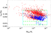 |
Fig. 1. M500–θ500 phase space of eROSITA EDR clusters (blue disks), shown in comparison to MCXC clusters (red circles), with boundaries demarcating the four equal-sized mass bins (vertical dashed lines) and the ten excluded θ500 < 1′ clusters (horizontal dot-dashed lines). |
Figure 2 presents the X-ray FX flux histogram in the [0.2, 2.3] keV single-detection band (we used this band in the rest of the study unless stated otherwise) of all the 27 910 likelihood ℒ ≥ 6 EDR catalog sources and of the subset of the 541 extended sources. We focused on the regime between the minimal flux of the extended-source distribution, Fmin ≃ 10−13.57 erg s−1 cm−2, which approximately coincides with the mean flux (Fmean) of the full sample, and the upper cutoff, Fmax ≃ 10−12 erg s−1 cm−2, imposed to avoid the apparent bright outliers. This range comprises 5820 sources, 534 of which are extended. We further separated this subsample into faint and bright sources using the threshold Fth ≃ 10−13 erg s−1 cm−2, which approximately coincides with the extended-source median. The ∼10″ resolution of the source catalog (adopting the camera pixel size; Brunner et al. 2022) is sufficient for the analysis of θ500 ≳ 1′ clusters.
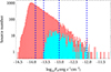 |
Fig. 2. Nominal ([0.2, 2.3] keV) flux distributions of extended (lower, cyan histogram) and all (higher, pink histogram) EDR catalog sources, with vertical dashed lines showing (from left to right) the flux levels of the full-catalog median, the mean (Fmean ≃ Fmin), the threshold (Fth), and the upper cutoff (Fmax). |
3. Binning and stacking
Denoting 𝒩(τ, c) as the number of sources found in a radial ring of normalized radius τ and width Δτ around cluster 1 ≤ c ≤ Nc, and ℱ(τ, c) as the number of combined foreground and background sources (henceforth field sources) expected in this ring, we adopted the field-only, 𝒩 = ℱ null hypothesis. A positive 𝒩 > ℱ excess is assigned a source-weighted (SW) significance
or a cluster-weighted (CW) significance
in the ℱ ≫ 1 normal-distribution limit. Modifications for a Poisson distribution, necessary for finite and especially small ℱ, are provided in Appendix A and incorporated henceforth.
For simplicity, given the EDR limited field of view, intermediate Galactic latitudes (20° ≲ b ≲ 40°), and large exposure variations, especially in the field periphery (Brunner et al. 2022), we approximated ℱ as a constant, measured in the {130° < RA < 142°, 0° < Dec < 4°} rectangle of fairly uniform exposure. The results are not sensitive to reasonable changes in the determination of ℱ(τ), including field estimates in the vicinity of each cluster and polynomial sky fits (see I24). We adopted the same nominal Δτ = 0.25 resolution used in previous stacking analyses. No substantial systematic errors are found when comparing SW to CW stacking, when varying the analysis parameters, or when analyzing, for each parameter set, > 105 control samples, each analogous to a real sample but with randomized cluster sky coordinates. A discussion of systematic effects and deviations from circular symmetry is available in I24.
Away from the central τ ≲ 1 excess of sources associated with the intracluster medium (ICM), the extended (respectively, extended and bright) sources present a > 3σ excess (respectively, > 2σ) inside the anticipated VS radius, peaked at 1.75 < τ < 2.0 (respectively, 2.0 < τ < 2.25), as shown in Fig. 3 (top row). Also incorporating non-extended EDR sources yields a local 2.0 < τ < 2.25 excess in each mass bin (1–4), although the low-mass bin (bin 1) shows only a ∼0.5σ excess, as compared to S > 2 in each of the more massive bins (2–4); the co-added excess over these three bins, shown in Fig. 3 (bottom row), presents a ∼3σ (respectively, ∼4σ) excess for all sources (respectively, for bright sources only). Results for each mass bin and for all bins combined are shown in Appendix C. We note that while the VS signal emerges in extended or bright sources without any cuts, it vanishes if Fmin is lowered, for example to the catalog median, which is sensitive to the ℒ cut.
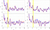 |
Fig. 3. Top row: significance, S(τ), radial profiles of all (left panel) or only bright F > Fth (right) extended eROSITA sources, SW (blue diamonds, with solid lines to guide the eye) or CW (red circles, with dashed lines) stacked around massive clusters (bins 2–4). Also shown are the Poisson-statistics confidence levels (±{1σ, 2σ, 3σ, …}; dotted black curves), the control-sample median and the corresponding containment fractions (50%,16%,2.3%,… for SW; dot-dashed green lines), and the anticipated 2.2 < τ < 2.5 VS region (vertical yellow shading) based on previous stacked γ-ray (RK18) and radio (H23) continuum and discrete X-ray and radio source detections (I24). Bottom row: same as the top panels, but also including non-extended sources in the same Fmin < F < Fmax range. |
The peripheral location of the excess and its proximity to the previously stacked signals tie it to the VS region. The narrowness of the signal indicates that the excess sources are directly associated with the shock, rather than being driven by the gradual changes in environment as infalling objects approach the cluster. The same findings in the ROSAT–MCXC analysis, along with the properties of the excess X-ray and radio sources, led us to the conclusion that these objects are likely shocked infalling gaseous halos, probably around galaxies or galaxy aggregates (I24). The VS excess typically peaks in the 2.0 < τ < 2.25 bin for EDR stacking, just inside the 2.25 < τ < 2.5 bin of maximal MCXC-stacking excess. This small offset might arise from differences in the catalog prescriptions for the R500 determination, although some redshift dependence cannot be ruled out.
4. Excess source properties
Although the localized 2.0 < τ < 2.25 (henceforth the VS bin) excess is significant, the number of excess sources is small compared to the coincident field sources, so we are unable to tie individual sources to the VS. We can, however, characterize the excess sources statistically, despite the small sample size, by comparing catalog properties in the VS bin and in the field.
We can consider some source properties, ℙ, of interest, such as the source extent (SE) or luminosity (L). In the absence of source redshifts, we estimated ℙ by assigning sources the redshift of their tentative host cluster. We then compared the differential (ℕ(ℙ)≡dN/dℙ) and cumulative (N(< ℙ)) distributions among the 𝒩(2.0 < τ < 2.25, c) sources in the VS bin (subscript V) to the distributions of many random samples, each of ℱ(2.0 < τ < 2.25, c) sources, drawn from the field region (subscript F). The cumulative VS excess, NV(< ℙ)−NF(< ℙ), and its local significance, S(ℙ) = [ℕV − μ(ℕF)]/σ(ℕF), were then estimated. We also examined a reference ICM region, 1.0 < τ < 1.5, rescaling its 𝒩 to the solid angle of the VS bin.
Figure 4 presents the SE distribution in the VS bin as compared to the field and ICM regions. There is a significant (> 3σ) local excess of ∼7 sources with 60 kpc ≲ SE ≲ 300 kpc, broadly consistent4 with the results from I24. The ICM region shows a comparable or slightly smaller SE, also based on only a few sources. The results in this section are based on bright (F > Fth) sources around clusters in mass bins 2–4 (which show the most significant excess in Fig. 3), but similar results are obtained for the entire sample with all mass bins (see Appendix B).
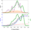 |
Fig. 4. SE distribution for nominal cuts (F > Fth and mass bins 2–4). Differential distributions (ℕ(ℙ); top panel) and cumulative distributions (N(< ℙ); bottom panel, left axis) are shown for ℙ = log10SE in the VS bin (solid and dot-dashed green lines), ICM region (double dot-dashed purple), field sampling (dotted red; pink-shaded 1σ dispersion), and VS excess (dashed blue). The bottom panel also shows the local significance, S(ℙ), of the VS excess (solid green curve, right axis). |
Low-redshift VS sources of LX ∼ 1042 − 43 erg s−1 luminosities were identified by I24 as thermal emission from shocked infalling halos, so one could naively expect LX ∝ (1 + z)6 luminosities ∼10 times higher at typical EDR redshifts, in both nominal and higher-energy bands. Figure 5 presents the logarithmic distributions of the LX, Lh, and Lu luminosities in the observed [0.2, 2.3], [2.3, 5], and [5, 8] keV bands, respectively. A significant VS excess of ∼15 sources in the 1043 − 44 erg s−1 range is indeed found in LX and Lh, whereas no significant excess can be identified in Lu. These sources are thus consistent with thermal emission from gaseous objects compressed and heated to keV-scale temperatures by the VS (see Appendix B).
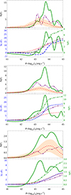 |
Fig. 5. Luminosity ℙ = log10L distributions in the [0.2, 2.3] (top two panels), [2.3, 5] (middle panels), and [5, 8] keV (bottom panels) bands, using the same sample and notations of Fig. 4. We have added a |
5. Summary and discussion
By stacking EDR sources (Fig. 2) around 532 EDR clusters (Fig. 1), we see a significant excess of extended (3σ) or bright (3.5σ) sources narrowly localized at normalized 2.0 < τ < 2.25 cluster radii (Figs. 3 and C.1). The proximity to the ROSAT–MCXC (I24) and other stacked signals directly links these sources to the VS shock of the host cluster and renders look-elsewhere corrections negligible. The sources are on average extended (Figs. 4 and B.1), with LX ≃ Lh ≃ 1043 − 44 erg s−1, which is about ten times higher than in the I24 sources, and no Lu detection (Figs. 5 and B.2), as expected for keV-scale sources at EDR redshifts. The signal strengthens (4σ) without the low-mass quartile, M500 < 1014.3, suggesting a host-mass dependence not seen by I24.
The stacked signals emerge thanks to the omission of faint background sources, F < Fmin ≃ Fmean (detected at lower likelihood levels), and the approximate similarity of clusters when scaled by R500. The small offset of the 2.0 < τ < 2.25 EDR signal from previous 2.2 < τ < 2.5 MCXC-based VS signals hints at a possible dependence on redshift or F cut, but could also arise from differences in the catalog prescriptions for R500 determination, which is based on X-rays in MCXC and weak lensing in EDR. Larger future studies could better resolve the offset and identify its origin, constrain the SE, L, and additional source properties, test the tentative M500 dependence, and examine deviations from spherical symmetry, which were suggested by I24 and earlier MCXC-based studies but are too weak for the EDR.
Our results are consistent with the tentative identification of the X-ray sources as thermal emission from gaseous objects, likely galactic halos, compressed and heated to keV-scale temperatures by the VS, with a strong LX(z) dependence. Their nonthermal counterpart, already seen as excess synchrotron radio sources, should also have nonthermal hard X-ray and possibly also γ-ray counterparts, so combining or cross-correlating broadband catalogs should uncover more VS-related phenomena (I24). We conclude that localized VS spikes in the distributions of discrete sources are a powerful probe of accretion from the cosmic web and of the underlying physical processes, ranging from the evolution of large-scale structure, to magnetization by the VS, to its dark matter splashback counterpart.
The EDR SE, defined as the core radius in a β = 2/3 model (Brunner et al. 2022), cannot be directly compared to ROSAT source radii (I24).
Acknowledgments
This research received funding from ISF grant No. 2126/22. May Gideon Ilani’s memory be a blessing.
References
- Anbajagane, D., Chang, C., Jain, B., et al. 2022, MNRAS, 514, 1645 [NASA ADS] [CrossRef] [Google Scholar]
- Bahar, Y. E., Bulbul, E., Clerc, N., et al. 2022, A&A, 661, A7 [NASA ADS] [CrossRef] [EDP Sciences] [Google Scholar]
- Brunner, H., Liu, T., Lamer, G., et al. 2022, A&A, 661, A1 [NASA ADS] [CrossRef] [EDP Sciences] [Google Scholar]
- Hou, K.-C., Hallinan, G., & Keshet, U. 2023, MNRAS, 521, 5786 [NASA ADS] [CrossRef] [Google Scholar]
- Hurier, G., Adam, R., & Keshet, U. 2019, A&A, 622, A136 [NASA ADS] [CrossRef] [EDP Sciences] [Google Scholar]
- Ilani, G., Hou, K.-C., & Keshet, U. 2024, arXiv e-prints [arXiv:2402.16946] [Google Scholar]
- Keshet, U., & Reiss, I. 2018, ApJ, 869, 53 [Google Scholar]
- Keshet, U., Kushnir, D., Loeb, A., & Waxman, E. 2017, ApJ, 845, 24 [NASA ADS] [CrossRef] [Google Scholar]
- Keshet, U., Reiss, I., & Hurier, G. 2020, ApJ, 895, 72 [NASA ADS] [CrossRef] [Google Scholar]
- Liu, A., Bulbul, E., Ghirardini, V., et al. 2022, A&A, 661, A2 [NASA ADS] [CrossRef] [EDP Sciences] [Google Scholar]
- Piffaretti, R., Arnaud, M., Pratt, G. W., Pointecouteau, E., & Melin, J.-B. 2011, A&A, 534, A109 [NASA ADS] [CrossRef] [EDP Sciences] [Google Scholar]
- Pratt, C. T., Qu, Z., & Bregman, J. N. 2021, ApJ, 920, 104 [NASA ADS] [CrossRef] [Google Scholar]
- Reiss, I., & Keshet, U. 2018, JCAP, 2018, 010 [Google Scholar]
- Reiss, I., Mushkin, J., & Keshet, U. 2017, Proc. 7th Int. Fermi Symp., (Garmisch-Partenkirchen, Germany), IFS2017, https://pos.sissa.it/cgi-bin/reader/conf.cgi?confid=312, 163 [Google Scholar]
Appendix A: Stacking equations
For a Poisson distribution of mean λ, where measurement k has probability p(k) = e−λλk/k!, we can analytically sum the probabilities of equal or larger (respectively smaller) k values to quantify the significance of a positive excess (respectively a negative deficit) in units of Gaussian standard errors,
![$$ \begin{aligned} S_p(k;\lambda ) = {\left\{ \begin{array}{ll} \sqrt{2}\,\mathrm{erfc}^{-1}\left[\frac{\Gamma (k)-\Gamma (k,\lambda )}{\Gamma (k)/2}\right]>0&\mathrm{if }~k>\lambda \,; \\ -\sqrt{2}\,\mathrm{erfc}^{-1}\left[\frac{\Gamma (1+k,\lambda )}{\Gamma (1+k)/2}\right]<0&\mathrm{if }~k < \lambda \,; \\ 0&\mathrm{if }~k=\lambda \,, \end{array}\right.} \end{aligned} $$](/articles/aa/full_html/2024/06/aa49819-24/aa49819-24-eq4.gif)
where erfc(x) and Γ(x) are respectively the complementary error and the Euler Gamma functions. One can find SSW for given Sp and ℱ by solving (cf. Eq. 1)

which results in the SSW(τ) profiles shown for integer Sp values in the S(τ) in Figs. 3 and C.1.
Appendix B: Source properties in the full sample
Figures B.1 and B.2 complement Figs. 4 and 5, respectively, showing the properties of all Fmin < F < Fmax sources around clusters in all mass bins. The signals are stronger here (i.e., they involve more excess sources than in Figs. 4 and 5) but are noisier. Regardless, our conclusions are qualitatively unchanged.
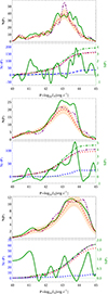 |
Fig. B.2. Luminosity distributions of all sample sources around all clusters (same notations as in Fig. 5). |
Appendix C: Mass dependence
Figure C.1 presents the stacked S(τ) profile in each of the four mass bins shown in Fig. 1, as well as the signal co-added over all four mass bins. While the higher-mass bins (2–4) each present a ∼2σ excess in the VS bin, the M ≲ 1014.3 clusters in mass bin 1 show a negligible excess. This result differs from the comparable signals found by I24 in all their mass bins; however, due to the poor statistics of the present sample, we cannot conclude that there is a meaningful difference between the EDR and ROSAT–MCXC results in this regard.
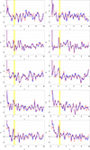 |
Fig. C.1. Same as Fig. 3, but showing mass bins 1–4 separately (first four panels, top down) and combined (bottom panel). |
All Figures
|
Fig. 1. M500–θ500 phase space of eROSITA EDR clusters (blue disks), shown in comparison to MCXC clusters (red circles), with boundaries demarcating the four equal-sized mass bins (vertical dashed lines) and the ten excluded θ500 < 1′ clusters (horizontal dot-dashed lines). |
| In the text | |
|
Fig. 2. Nominal ([0.2, 2.3] keV) flux distributions of extended (lower, cyan histogram) and all (higher, pink histogram) EDR catalog sources, with vertical dashed lines showing (from left to right) the flux levels of the full-catalog median, the mean (Fmean ≃ Fmin), the threshold (Fth), and the upper cutoff (Fmax). |
| In the text | |
|
Fig. 3. Top row: significance, S(τ), radial profiles of all (left panel) or only bright F > Fth (right) extended eROSITA sources, SW (blue diamonds, with solid lines to guide the eye) or CW (red circles, with dashed lines) stacked around massive clusters (bins 2–4). Also shown are the Poisson-statistics confidence levels (±{1σ, 2σ, 3σ, …}; dotted black curves), the control-sample median and the corresponding containment fractions (50%,16%,2.3%,… for SW; dot-dashed green lines), and the anticipated 2.2 < τ < 2.5 VS region (vertical yellow shading) based on previous stacked γ-ray (RK18) and radio (H23) continuum and discrete X-ray and radio source detections (I24). Bottom row: same as the top panels, but also including non-extended sources in the same Fmin < F < Fmax range. |
| In the text | |
|
Fig. 4. SE distribution for nominal cuts (F > Fth and mass bins 2–4). Differential distributions (ℕ(ℙ); top panel) and cumulative distributions (N(< ℙ); bottom panel, left axis) are shown for ℙ = log10SE in the VS bin (solid and dot-dashed green lines), ICM region (double dot-dashed purple), field sampling (dotted red; pink-shaded 1σ dispersion), and VS excess (dashed blue). The bottom panel also shows the local significance, S(ℙ), of the VS excess (solid green curve, right axis). |
| In the text | |
|
Fig. 5. Luminosity ℙ = log10L distributions in the [0.2, 2.3] (top two panels), [2.3, 5] (middle panels), and [5, 8] keV (bottom panels) bands, using the same sample and notations of Fig. 4. We have added a |
| In the text | |
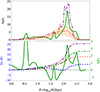 |
Fig. B.1. SE distribution of all sample sources around all clusters (same notations as in Fig. 4 |
| In the text | |
|
Fig. B.2. Luminosity distributions of all sample sources around all clusters (same notations as in Fig. 5). |
| In the text | |
|
Fig. C.1. Same as Fig. 3, but showing mass bins 1–4 separately (first four panels, top down) and combined (bottom panel). |
| In the text | |
Current usage metrics show cumulative count of Article Views (full-text article views including HTML views, PDF and ePub downloads, according to the available data) and Abstracts Views on Vision4Press platform.
Data correspond to usage on the plateform after 2015. The current usage metrics is available 48-96 hours after online publication and is updated daily on week days.
Initial download of the metrics may take a while.