| Issue |
A&A
Volume 686, June 2024
|
|
|---|---|---|
| Article Number | A60 | |
| Number of page(s) | 13 | |
| Section | Cosmology (including clusters of galaxies) | |
| DOI | https://doi.org/10.1051/0004-6361/202449143 | |
| Published online | 30 May 2024 | |
GLACE survey: OSIRIS/GTC tuneable imaging of the galaxy cluster ZwCl 0024.0+1652
II. The mass–metallicity relationship and the effect of the environment
1
Institut de Radioastronomie Millimétrique (IRAM), Av. Divina Pastora 7, Núcleo Central, 18012 Granada, Spain
e-mail: This email address is being protected from spambots. You need JavaScript enabled to view it.
2
Asociación Astrofísica para la Promoción de la Investigación, Instrumentación y su Desarrollo, ASPID, 38205 La Laguna, Tenerife, Spain
3
Centro de Astrobiología (CSIC/INTA), ESAC Campus, 28692 Villanueva de la Cañada, Madrid, Spain
4
ISDEFE for European Space Astronomy Centre (ESAC)/ESA, PO Box 78 28690 Villanueva de la Cañada, Madrid, Spain
5
Instituto de Astrofísica de Canarias (IAC), 38200 La Laguna, Tenerife, Spain
6
Departamento de Astrofísica, Universidad de La Laguna (ULL), 38205 La Laguna, Tenerife, Spain
7
Departamento de Física de la Tierra y Astrofísica, Instituto de Física de Partículas y del Cosmos, IPARCOS, Universidad Complutense de Madrid (UCM), 28040 Madrid, Spain
8
Instituto de Física de Cantabria (CSIC-Universidad de Cantabria), 39005 Santander, Spain
9
Instituto de Astronomía, Universidad Nacional Autónoma de México, Apdo. Postal 70-264, 04510 Ciudad de México, Mexico
10
Fundación Galileo Galilei-INAF, Rambla José Ana Fernández Pérez, 7, 38712 Breña Baja, Tenerife, Spain
11
Centro de Estudios de ísica del Cosmos de Aragón (CEFCA), Plaza San Juan 1, 44001 Teruel, Spain
12
Space Science and Geospatial Institute (SSGI), Entoto Observatory and Research Center (EORC), Astronomy and Astrophysics Research Division, PO Box 33679 Addis Abbaba, Ethiopia
13
Instituto de Astrofísica de Andalucía (CSIC), 18080 Granada, Spain
14
Physics Department, Mbarara University of Science and Technology (MUST), Mbarara, Uganda
15
Addis Ababa University (AAU), PO Box 1176 Addis Ababa, Ethiopia
16
Physics Department, Kotebe Metropolitan University (KMU), PO Box 31248 Addis Ababa, Ethiopia
17
Telespazio Vega UK for ESA, European Space Astronomy Centre, Operations Departmen, 28691 Villanueva de la Cañada, Spain
Received:
2
January
2024
Accepted:
26
February
2024
Abstract
Aims. In this paper, we revisit the data for the galaxy cluster ZwCl 0024.0+1652 provided by the GLACE survey and study the mass–metallicity function and its relationship with the environment.
Methods. Here we describe an alternative way to reduce the data from OSIRIS tunable filters. This method gives us better uncertainties in the fluxes of the emission lines and the derived quantities. We present an updated catalogue of cluster galaxies with emission in Hα and [N II] λλ6548,6583. We also discuss the biases of these new fluxes and describe the way in which we calculated the mass–metallicity relationship and its uncertainties.
Results. We generated a new catalogue of 84 emission-line galaxies with reliable fluxes in [N II] and Hα lines from a list of 174 galaxies. We find a relationship between the clustercentric radius and the density of galaxies. We derived the mass–metallicity relationship for ZwCl 0024.0+1652 and compared it with clusters and field galaxies from the literature. We find a difference in the mass–metallicity relationship when compared to more massive clusters, with the latter showing on average higher values of abundance. This could be an effect of the quenching of the star formation, which seems to be more prevalent in low-mass galaxies in more massive clusters. We find little to no difference between ZwCl 0024.0+1652 galaxies and field galaxies located at the same redshift.
Key words: ISM: abundances / galaxies: clusters: individual: ZwCl 0024.0+1652 / galaxies: star formation / cosmology: observations
© The Authors 2024
 Open Access article, published by EDP Sciences, under the terms of the Creative Commons Attribution License (https://creativecommons.org/licenses/by/4.0), which permits unrestricted use, distribution, and reproduction in any medium, provided the original work is properly cited.
This article is published in open access under the Subscribe to Open model. This email address is being protected from spambots. You need JavaScript enabled to view it. to support open access publication.
1. Introduction
The evolution of the star formation process in cluster galaxies is still an open field. The pioneering works of Gisler (1978) and Dressler et al. (1985) established that emission-line galaxies (ELGs) are more numerous in the field than in clusters. Other works have delved deeper into the issue: for example Balogh et al. (1997) found that cluster galaxies are likely to have less significant star formation processes than field galaxies, finding that the star formation rate (SFR) in cluster galaxies is lower when compared with field galaxies; Cucciati et al. (2010) and Cantale et al. (2016) reported that the fraction of blue galaxies is significantly lower in groups than in field galaxies; Allen et al. (2016) found that the mass-normalised SFR for the highest-mass galaxies in the field was larger than for galaxies in clusters; Old et al. (2020) found that the star-forming main sequence for galaxies in clusters is lower compared to that of the field galaxies, and this effect was more significant for lower-mass galaxies; and Vaughan et al. (2020) found that the average Hα-to-continuum-size ratio of ELGs is smaller in cluster galaxies than in field galaxies with the same stellar mass.
The reasons for these differences may be associated with the quenching of star formation in cluster galaxies. Boselli & Gavazzi (2006) list the possible causes in their review: starvation (removal of the outer galaxy halo that feeds the star formation, preventing further infall of gas into the disc (Larson et al. 1980); ram-pressure stripping (removal of the galactic gas by moving at high velocities in dense and hot intergalactic medium (Gunn & Gott 1972); or harassment (interactions of the galaxy with the potential of the cluster as a whole (Moore et al. 1996), among others.
Metallicities have been found to be affected by this quenching (see Darvish et al. 2015). There is a tight correlation between the abundance of galaxies and their stellar mass: the more massive the galaxy, the higher the metallicity. This is called the mass–metallicity relationship (hereafter, MZR). As proposed by Lara-López et al. (2010), this relationship may be an indicator of a more profound link between metallicity, stellar mass, and SFR, which has been referred to as the “fundamental plane”.
It is assumed that pristine gas falls into galaxies and is then turned into stars and released at the end of the life of the massive stars. Some of this gas, enriched with metals, may escape the gravity well of its parent galaxy. However, in more massive galaxies with larger gravity wells, this gas will have a lesser tendency to escape when compared with galaxies of lower masses. Therefore, in general, in the absence of interactions with other galaxies, this may imply that galaxies with larger stellar masses will be more metallic. Following this criterion, the MZR may be influenced by the environment: galaxies located within the denser areas of a cluster could potentially be subject to a greater number of interactions than field galaxies or galaxies in the outskirts of the same cluster. These interactions may strip galaxies of their less metallic gas by some of the processes mentioned above, and these galaxies will therefore have a higher metallicity content than those in the field or in less dense environments (see e.g. Maier et al. 2019, and references therein). The MZR has been described in many different contexts; for example, in field galaxies in the local Universe (Tremonti et al. 2004; Lee et al. 2006 or Andrews & Martini 2013, among others), in field galaxies at higher redshifts (i.e. Calabrò et al. 2017 for 0.1 < z < 0.9 or Hayashi et al. 2009 for up to z ∼ 2), and in galaxies in clusters (see e.g. Sobral et al. 2016; Ciocan et al. 2020; Maier et al. 2019; Lara-López et al. 2022 or Pérez-Martínez et al. 2023, among others).
Here, we present a revisiting of the cluster ZwCl 0024.0+1652 (hereafter Cl0024) using improved reduction techniques. The paper is organised as follows. In Sect. 2, we describe the GLACE survey, explain the inverse convolution method, and present the galaxy cluster Cl0024. In Sect. 3, we discuss the way we parameterised the environment. Section 4 is devoted to the MZR for Cl0024, where we also present a comparison with other clusters and field galaxies from the literature. In Sect. 5 we discuss our main results and present the conclusions of this work. Throughout this paper, we assume a standard Λ-cold dark matter cosmology with ΩΛ = 0.7, Ωm = 0.3, and H0 = 70 km s−1 Mpc−1.
2. The GLACE survey: Revisiting the pseudospectra
The GLACE (GaLAxy Cluster Evolution Survey) is a narrow-band survey of ELGs and AGNs in a sample of galaxy clusters located at different redshifts. The aim of GLACE is to study the variations in galaxy properties as a function of environment. The main objectives and methods of this survey are described in detail in Sánchez-Portal et al. (2015). Briefly, GLACE was developed as the cluster counterpart of the OTELO survey (Bongiovanni et al. 2019), observing clusters at z ∼ 0.4, 0.63, and 0.86, and mapping several rest-frame optical emission lines, such as Hα, Hβ, [N II], [O II]λ3727, and [O III]λ5007.
We selected Cl0024 from the lower redshift observations; it has a precise redshift of z = 0.395. We obtained data through tunable filter tomography, employing the instrument OSIRIS on the 10.4 m GTC (Gran Telescopio Canarias) at Roque de los Muchachos Observatory. The whole process of obtaining and reducing the data is described in Sánchez-Portal et al. (2015). Briefly, the data were obtained through the technique of TF tomography (Cepa et al. 2013), where a series of tuned images were obtained, sampling the [N II] and Hα lines. The result is a pseudospectrum for each ELG. This pseudospectrum is a convolution of the real spectrum of the ELG with the response function of the OSIRIS instrument. A total of 174 ELGs were detected from the cluster. From there, fluxes from the Hα, and [N II] lines were derived, as well as redshifts. AGNs were detected and marked as such (see Sánchez-Portal et al. 2015 for details).
2.1. The inverse convolution method
The method to derive the fluxes and their uncertainty for the 174 ELGs is detailed in Eqs. (10) and (11) of Sánchez-Portal et al. (2015); in Eq. (11), the uncertainty is obtained using a first-order approximation of the variance in uncertainty propagation theory. However, such first-order approximations lead to larger, unrealistic variance estimates, especially when ratios of quantities are used and the nominal variances of the quantities involved have an associated relative standard deviation of greater than 10% (as is the case in Eq. (10) of Sánchez-Portal et al. 2015). Worse yet, for large relative standard deviations, not only is the uncertainty overestimated, but the nominal value of the inferred quantity is also biased if ratios or logarithm operations are involved (see Cerviño & Valls-Gabaud 2003, for a case of study for different inference types).
Fortunately, since this first iteration with the data, a new method to obtain the fluxes from the pseudospectra has been developed. This latter is based on a Monte Carlo sampling of the multi-parametric probability distribution function (PDF) of the intensity of the continuum fluxes and the shape of the principal lines in the pseudo-spectrum produced by the tunable filters. The multi-parametric PDFs are also used to obtain the associated PDFs of line ratios and related quantities, such as metallicities, and this approach has been employed in several works related to the OTELO Survey (i.e. Bongiovanni et al. 2020; Nadolny et al. 2020; Cedrés et al. 2021; Navarro Martínez et al. 2021).
This method, named “inverse convolution”, is described in detail in Appendix A of Nadolny et al. (2020). Briefly, a model spectrum as a rest-frame spectrum is simulated by Gaussian profiles of the [N II] and Hα lines defined by their amplitude, common line width for three lines, and a constant continuum level. The model is then convolved with the spectral response of the OSIRIS instrument and then compared with the observational data through a likelihood function. This is repeated a total of 105 times. After this process, we obtain a PDF shape for each parameter, as well as all the required additional quantities. This allows us to obtain more reliable values for the Hα and [N II] fluxes, which will lead to more informed estimates of the metallicity. The inverse convolutions can be used to derive the redshift, the continuum, the fluxes of the lines (Hα, [N II]λ6548 and [N II]λ6583 in this case), and the full width at half maximum (FWHM) of the lines. The uncertainties can be directly obtained from the PDF. In our case, we use the 68% confidence interval around the mode of the PDF for each parameter.
This new way of obtaining the fluxes from the emission lines allows us to revisit the data from Cl0024 and study its properties in greater detail. The results can be seen in Fig. 1, where present the pseudospectrum of the galaxy id:424 (upper panel) and the deconvolved spectrum (lower panel) as well as the 68% confidence interval of the fit.
 |
Fig. 1. Pseudospectrum with fitting components (upper panel) and deconvolved spectrum (lower panel) for the tier 1 galaxy id:424. The filled grey area represents the 68% confidence interval. |
After all the galaxies from Sánchez-Portal et al. (2015) were reprocessed by the inverse convolution method, a classification of the fitted spectra – based on careful visual inspection – was carried out, taking into account the quality of the deconvolution as well as the uncertainties. In this new classification, the galaxies were sorted into tiers. Tiers 1 to 3 are well-deconvolved galaxies, with galaxies from tier 1 having the smallest uncertainties and those from tier 3 galaxies having the largest. We also made sure that all fluxes, redshifts, and derived quantities present PDFs that can be approximated as Gaussians. This means that the mode, median, and mean of the PDFs are very close, and so we can use any of them interchangeably. From the total of 174 galaxies by Sánchez-Portal et al. (2015), we derived reliable fluxes for 84 of them. For the remaining galaxies, in 47 cases we were unable to separate the [N II] lines from the Hα, line, 16 cases presented a complex Hα, line made up of several superimposing components, and in 27 cases the algorithm did not converge. Of the cases with a composite Hα, line and those for which we were unable to separate Hα, and [N II] lines, 75% and 30% are classified as AGNs by Sánchez-Portal et al. (2015) respectively. Table 1 contains a summary of the classification for all the galaxies. In Table A.1, we present the results of the inverse convolution for the 84 galaxies from tiers 1 to 3, indicating the Hα and [N II]λ6584 fluxes as well as the metallicity. Hereafter, unless otherwise stated, we only analyse and discuss galaxies from tiers 1 to 3.
Number of galaxies in the sample segregated by quality.
2.2. Galaxy cluster ZwCl 0024.0+1652
Cl0024 is a galaxy cluster located at mid-redshift (z ∼ 0.4); it has been described as having a rather complex structure that does not appear at visible wavelengths (Czoske et al. 2002), and is low in X-ray flux and central velocity dispersion (Johnson et al. 2016). Cl0024 is one of the original clusters of the pioneering paper by Butcher & Oemler (1978), where the so-called Butcher–Oemler effect was first described. Beyoro-Amado et al. (2021) reported that the core is almost totally made up of early-type galaxies with no emission lines up to ∼500 kpc, with increasing numbers of late-type galaxies in the outskirts. Sánchez-Portal et al. (2015) suggest that this seems to indicate a quenching of star formation and AGN activity.
The cluster has been divided into at least two substructures by several authors (i.e. Czoske et al. 2002; Moran et al. 2007; Sánchez-Portal et al. 2015): one that constitutes the main cluster and centred at z = 0.395 (thereafter Structure A) and a second group of infalling galaxies at z = 0.381 (thereafter Structure B). Czoske et al. (2002) suggest that these two structures are colliding along the line of sight. Moreover, Czoske et al. (2002) and Sánchez-Portal et al. (2015) propose the existence of a third interacting structure at about z ∼ 0.42.
In the upper panel of Fig. 2, we show the distribution of redshifts derived from the inverse convolution method (solid black line) and the redshifts from Sánchez-Portal et al. (2015) (blue dashed line). The two structures are clearly identified in the histogram. Moreover, the proposed third structure can be seen at z ∼ 0.42. The lower panel shows the residuals between the new and the old determination. The coincidence between both methods is very good, with the majority of the galaxies presenting differences of less than 0.001 in redshift.
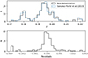 |
Fig. 2. Redshift distribution for the galaxies presented in this study of Cl0024. The upper panel shows the distribution of redshifts derived from the new determination (solid line) and the determination from Sánchez-Portal et al. (2015) (dashed line). The lower panel shows the distribution of the residuals between the old and the new redshift determination. This figure includes all the galaxies (tiers 1 to 3, and “no deblending” and “composite Hα, lines”). |
Figure 3 shows the Hα flux derived from the inverse convolution method versus the Hα flux derived from Sánchez-Portal et al. (2015). There is a very good correlation between the results of the two methods (as expected). Nevertheless, it seems that the determination by Sánchez-Portal et al. (2015) has marginally higher values when compared with those from the inverse convolution method.
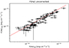 |
Fig. 3. Comparison between the obtained values for the Hα emission line uncorrected for extinction from Sánchez-Portal et al. (2015) and the new one from this work. The red continuous line indicates a 1:1 relation. |
On the other hand, the real strength of the inverse convolution method is shown in Fig. 4 where it is compared to the distribution of the relative uncertainties obtained by Sánchez-Portal et al. (2015) and the new ones, defined as the 68% confidence interval. The median value of the distribution of relative uncertainties in the Hα flux from the Sánchez-Portal et al. (2015) determination is above 20%, while with the inverse convolution method is just over 10%, with many galaxies having uncertainties in the Hα line at 5% and below. This difference allows us to calculate all the derived quantities (such as the abundance) with enough precision to to make robust conclusions.
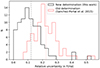 |
Fig. 4. Histogram of the relative uncertainty in the flux determination in the Hα line. The red histogram is the error from Sánchez-Portal et al. (2015). The red dotted line is the median value of the relative error. The black histogram is the relative error from this work. The grey dashed line represents the median value. |
3. Parameterisation of the environment
We characterise the local environment of our sample by applying a modified version of the method first described in Dressler (1980). We calculated the projected surface density of the galaxies in our data set, estimated as the source density in the area encircled between the object and the tenth nearest galaxy above a certain magnitude threshold (Σ10) according to the following equation:
 (1)
(1)
where R10 is the projected distance in megaparsecs from the considered galaxy to the tenth closest object. In this case, we take objects brighter than I ∼ 21.5 measured in GLACE ancillary data (Sánchez-Portal et al. 2015), where the completeness of the spectroscopic member catalogue is above 70% along the full area covered by the observations (Perez-Martinez et al., in prep.). We also take into account the two main structures described in Sect. 2.
Figure 5 shows the logarithm of the Σ10 as a function of the clustercentric radius for all galaxies from Sánchez-Portal et al. (2015). We take the centre of the cluster to be that suggested in Sánchez-Portal et al. (2015). The median values for the Structures A and B galaxies are indicated by the grey dashed line and the red dashed line, respectively. A tight correlation exists, with galaxies with a lower clustercentric radius having a larger value in log(Σ10). This is not surprising because, we expect to find a denser environment for galaxies in the inner parts of the cluster. The galaxies from the infall Structure show, in general, lower values in density when compared with galaxies in the main structure and can be clearly identified in Fig. 5. We note that the clustercentric radius used in this case originates from the centre of Structure A, and so, in principle, we would expect a greater scattering of galaxies in Structure B. However, the figure shows a tight correlation for those galaxies. This seems to indicate that the centres of the two structures must be relatively closely projected onto the sky, as suggested by Czoske et al. (2002).
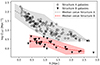 |
Fig. 5. Logarithm of Σ10 as a function of the clustercentric radius for all the galaxies from Sánchez-Portal et al. (2015). Open circles and downward-pointing filled triangles are the galaxies from Structures A and B, respectively. The grey and red dashed lines show the median value for galaxies in Structures A and B, respectively. The filled grey and red areas represent the median absolute deviation for Structures A and B, respectively. |
4. The mass–metallicity relationship
To determine the abundance of the ELGs of Cl0024, and keeping in mind that we are restricted to the Hα and [N II] lines, we employed the recipe given by Pettini & Pagel (2004) using the ratio N2. This ratio is defined as
![Mathematical equation: $$ \begin{aligned} \mathrm{N2}\equiv \log \left(\frac{\left[{\mathrm{N}\,\text{\small{II}} }\right]\lambda 6583}{\mathrm{H}\alpha }\right)\cdot \end{aligned} $$](/articles/aa/full_html/2024/06/aa49143-24/aa49143-24-eq2.gif) (2)
(2)
Then, the metallicity is derived using the following equation:
 (3)
(3)
No extinction correction is necessary given the proximity in wavelength of the two lines (Hα and [N II]λ6583). To avoid the systematic effect of different abundance calibrations, when comparing the MZR with data from the literature, all the metallicities presented in this work are calculated using the N2 method. We only calculated the abundance for galaxies marked as star-forming galaxies in the catalogue presented in Sánchez-Portal et al. (2015), taking out all those classified as AGNs.
We obtained stellar mass estimations for star-forming galaxies by modelling SEDs based on the broad-band (BVRIJKs), publicly available optical and near-infrared data described by Moran et al. (2005), and fixing redshift to the values derived from the inverse convolution method. We used a set of low-resolution, composite stellar population templates with delayed exponential star formation histories (SFHs) obtained from the stellar population synthesis models of Bruzual & Charlot (2003), adopting four stellar metallicity values (from Z = 0.0004 to Z⊙; Padova 1994 tracks) and an initial mass function (IMF) according to Chabrier (2003). The age of star formation was constrained to between 10 Myr and 10 Gyr (about the age of the Universe at the mean redshift of the cluster) and the e-folding times in the 0.01 < τ < 30 Gyr range. The best fit of the models was obtained using LePhare (Arnouts et al. 1999; Ilbert et al. 2006), assuming the Calzetti et al. (2000) extinction law with intrinsic reddenning E(B − V) varying between 0 and 0.5 mag. The median  value obtained from SED fitting is 1.57 and the medians of stellar mass estimations are distributed in the 8.4 ≤ log (M* [M⊙]) ≤ 11 range, with a mean uncertainty of about 0.3 dex. Those estimations are fully consistent with those obtained from exponentially declining SFH and the same prescriptions as those indicated above.
In order to make a meaningful comparison with other MZRs from the literature, we follow the recipe suggested by Curti et al. (2020), where the data were binned and fitted to the equation adapted from Zahid et al. (2014), which in turn is an evolution of the functional relationship presented in Moustakas et al. (2011):
 (4)
(4)
where according to Curti et al. (2020), M* is the stellar mass in solar masses; Z0 is the saturation metallicity, which gives the upper metallicity limit of the MZR; M0 is the turnover mass; and γ is the power law that controls the MZR at M* < M0. This fit is applied to binned data of log (M*). Curti et al. (2020) used 0.15 dex stellar mass bins. In order to improve the dispersion of the fits, we decided to fix the saturation abundance. According to Marino et al. (2013), the N2 ratio begins to saturate at N2 ≃ −0.4, meaning it no longer presents a linear relationship with oxygen abundance. This is equivalent to 12 + log(O/H) ∼ 8.67, and so we assume that this is the asymptotic metallicity of the MZR for galaxies with M* ≫ M0. In this way, the parameters to fit are reduced to two: the turnover mass M0, and the exponent of the power law γ.
To obtain the parameters of the fitting, a set of Monte Carlo simulations were carried out. Each galaxy had a simulated random value of log(M*) and of 12 + log(O/H) inside the uncertainty of both quantities of the given object. Then, a new MZR was constructed with these simulated values. After that, the MZR was binned in stellar mass. Due to our smaller number of galaxies in clusters at larger redshift, when compared with the Curti et al. (2020) set, our bins need to be larger in order to include a significant number of galaxies. In the end, we employed 0.62 dex stellar mass bins for our data. Also, this same binning was employed for all the comparison clusters from the literature. This process was repeated 100 000 times, resulting in a set of binned MZRs. Each binned MZR was then fitted using a least-squares minimisation algorithm based on the Levenberg–Marquardt method. The mean and standard deviation were calculated for all the fits. The mean was considered the best fit for the MZR, and the standard deviation was assumed to be the main uncertainty for the MZR. Moreover, the resultant parameters (M0 and γ) and their uncertainty were calculated as the mean of all the values obtained in every fit and its standard deviation, respectively.
In Fig. 6 we show the MZR for the ELGs detected in the cluster Cl0024. The grey dashed line represents the mean fitted Eq. (4). The filled grey area is the 1σ uncertainty on the fits. As expected, there is a tight correlation between the stellar mass and the metallicity of the galaxies, with lower-mass galaxies having lower values of oxygen abundance.
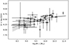 |
Fig. 6. MZR for the SFGs of Cl0024. Our data are the open circles, the black-dashed line represents the mean of the fitted values employing the recipe by Curti et al. (2020), and the grey area represents the 1σ deviation of the fits. |
In Table 2 we summarise the properties of the clusters used in this study. Table 3 lists the fit parameters of Eq. (4) for all the clusters, local SDSS galaxies in clusters, and field galaxies at z ∼ 0.4, which we use for comparison in the following sections.
Main characteristics of the galaxy clusters employed in this study.
4.1. The effect of the environment
Figure 7 shows the MZR for the galaxies of Cl0024. In the left panel, we only show the galaxies of the main structure inside 0.5 R200 (black open circles) and the galaxies of the infall group (red circles). In the right panel, we separate Cl0024 galaxies into medium and high-density zones, log(Σ10)≧1.7, following the criteria suggested by Sobral et al. (2016); these are represented by open red circles, and galaxies in low-density zones are represented by open black circles. In order to eliminate some of the noise in the figure, we only consider the galaxies with an uncertainty of 1% in the abundance determination.
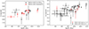 |
Fig. 7. MZR for Cl0024. Left panel: open black circles and red filled circles are the galaxies with R < 0.5 R200 and galaxies in Structure B, respectively. Right panel: open red circles and open black circles are the galaxies from Cl0024 within medium and high-density zones (log(Σ10)≧1.7) and low-density zones (log(Σ10) < 1.7), respectively. |
Maier et al. (2019) found that the galaxies with 0.5 R200 have enhanced metallicities when compared to the infall galaxies of the same cluster. However, we find no such differences between the infall group and the galaxies inside 0.5 R200. An explanation for this difference could be that XMMXCS J2215.9–1738 infall galaxies come from the field, and are therefore poorer in metals when compared with the galaxies from the core. On the other hand, the infall group in Cl0024 is, in reality, a subgroup of galaxies with a certain density above that of the field galaxies.
The right panel of Fig. 7 also shows that there is no difference between galaxies in high-density zones and those in low-density zones. All these results seem to agree with Sobral et al. (2016), who found no significant dependence of the MZR on the environment inside the same cluster.
Figure 8 shows the abundance as a function of the clustercentric radius for galaxies on Structures A and B. The median value is represented by a grey dashed line and only for galaxies in Structure A. This median value and its uncertainty were calculated in the same way as the binned median MZR was computed, as described in Sect. 4. The filled grey zone represents the uncertainty on the median value of 1σ. The blue dotted line represents the position of the Rvirial from Sánchez-Portal et al. (2015). There is a slight dependence of the metallicity on clustercentric radius, with inner galaxies presenting, at least on average, larger abundances. We find no clear differences between galaxies in Structures A and B. However, Maier et al. (2015) found that the metallicities of galaxies inside the virialized part of the cluster they studied presented enhanced metallicities by about 0.1 dex when compared to infalling galaxies. Here, the difference in median abundance between galaxies well inside the virialized part and galaxies in the outside zones is about ∼0.25 dex, which is slightly larger than the difference reported by Maier et al. (2015). This is a result similar to the one presented in Ellison et al. (2009), where it is reported that the galaxies are slightly more metal-rich if they are located in overdensity zones. Lara-López et al. (2022) also find a dependence of the metallicity on projected clustercentric radius for galaxies in the Fornax cluster. On the other hand, Mouhcine et al. (2007) and Cooper et al. (2008) found weak or no connection between abundance and environment in galaxies. However, Cooper et al. (2008) expanded the study, and after removing the mean colour–luminosity–environment relation, found a residual relationship between environment and metallicity.
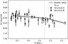 |
Fig. 8. Metallicity as a function of clustercentric radius for Cl0024. The open black circles are the galaxies from Structure A. The downward black-filled triangles are the galaxies from Structure B. The grey dashed line is the median of the values for Structure A. The blue dotted line indicates the position of the virial radius for Cl0024 from Sánchez-Portal et al. (2015). |
4.2. Effect of the mass of the cluster
In Fig. 9 we make a comparison with data from cluster RX J2248–4431 (thereafter RXJ2248) from Ciocan et al. (2020), cluster MACS J0415.1–2403 (thereafter MACS0415) from Maier et al. (2016), and cluster Cl 0939+4713 (thereafter Cl0939) from Sobral et al. (2016). All clusters are at a similar redshift.
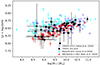 |
Fig. 9. Mass–metallicity relationship for ELGs in clusters at similar redshift. Black circles represent our data. The cyan downward-pointing triangles are the galaxies from Ciocan et al. (2020) for the cluster RX J2248–4431. The blue pentagons represent the galaxies from Sobral et al. (2016) for the cluster Cl 0939+4713. The red upward-pointing triangles are the galaxies from Maier et al. (2016) for the cluster MACS J0416.1–2403. |
Figure 10 shows the fitted functions described in Eq. (4) with one standard deviation (filled regions) of the MZR for the four clusters and the SDSS galaxy clusters (black thick line) from Tempel et al. (2017) at local redshift. It should be noted that all four clusters have been chosen in such a way that they are in a similar non-relaxed status (i.e. Sánchez-Portal et al. 2015; Czoske et al. 2002 for Cl0024; Schindler et al. 1998 for Cl0939; Mann & Ebeling 2012 for MACS0416; and Rahaman et al. 2021; Kesebonye et al. 2023 for RXJ2248). We can see that the fitted value of the abundance for RXJ2248 is systematically larger than the abundance for our data of Cl0024. On the other hand, the data from MACS0416 follow, inside uncertainties, the same path as Cl0024. The data from Cl0939 seem to follow a shallower path when compared with RXJ2248. However, the fact that the data from Sobral et al. (2016) do not include uncertainties should be taken into account. In the end, we decided to add a 5% error to each measured flux. Therefore, it is possible that, in this case, we are underestimating the total uncertainty of the fit. Nevertheless, the value of the abundance for Cl0939 is larger than Cl0024 for all ranges in stellar mass. Moreover, most of the time, the abundance fitted for RXJ2248 and Cl0939 is larger than or equal to that in local clusters, and the abundances for Cl0024 and MACS0416 are below them. If we take into account the fitted parameters presented in Table 3, we can see that the main difference between the clusters lies in the turnover mass, log(M0/M⊙), with Cl0024 and MACS0416 having a large value (10.68 and 10.46 respectively) when compared to Cl0939 and RXJ2248 clusters. This indicates that γ, the low-mass end slope, is dominant for almost all stellar masses sampled in Cl0024 and MACS0416. The shallow behaviour of Cl0939, represented by the low value of γ = 0.12 ± 0.008, may be due to the lack of low-stellar-mass galaxies when compared with the other two clusters, which generates a poor constraint when fitting. On the other hand, the γ obtained for Cl0024, RXJ2248, MACS0416, and local clusters are similar within the uncertainties.
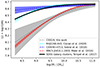 |
Fig. 10. Comparison of MZR between Cl0024 and clusters at the same redshift, as well as galaxies from clusters at low redshift from Tempel et al. (2017). The colour coding is reported in the legend. All data were fitted following the recipe presented in Curti et al. (2020). |
From Table 2, it can be seen that the M200 masses for RXJ2248 and Cl0939 are 2.81 × 10¹⁵ M⊙ and 1.7 × 10¹⁵ M⊙, respectively. Both are an order of magnitude higher than the reported mass for Cl0024. On the other hand, the M200 for MACS0416 is somewhat lower, less than two times larger than the mass for Cl0024.
According to Calabrò et al. (2017), the MZR is a consequence of the conversion of gas into stars inside galaxies, a process regulated by gas exchanges with the environment. There should therefore be a correlation between the total abundance of the gas in the galaxies and the metallicity of the intracluster gas. However, in Table 2 we can see that the average values of Z/Z⊙ for Cl0024, Cl0939, MACS0416, and RXJ2248 are similar.
Nevertheless, we have to take into account that the metallicity is not constant within each cluster, and here we are comparing average values. According to De Filippis et al. (2003), Cl0939 shows a high-metallicity region (they called it M1, with Z/Z⊙ ≃ 0.33) with a peak in galaxy number density. These authors suggest that the galaxies there may have enriched the gas in the zone compared with others with a lower galaxy number density. For RXJ2248, Rahaman et al. (2021) gives Z/Z⊙ ≃ 0.36 for the centremost zone of the cluster. On the other hand, Zhang et al. (2005) give a value of Z/Z⊙ ≃ 0.25 for the most metallic zone in Cl0024. If we take this into account, it is clear that Cl0939 and RXJ2248 show zones where the intracluster gas has larger abundances than the most metallic zone of Cl0024.
Figure 11 shows the logarithm of M0 as a function of M200 for all the clusters presented in Table 2. The filled black circle is the cluster Cl0024, and the open black circles are the clusters at about z ∼ 0.4. The open red triangles are the clusters at larger redshift. The filled black star represents the Hercules Supercluster at z ∼ 0.033. The figure indicates that the drive for the change in the turnover mass, and therefore in the larger abundance for several clusters, lies in the M200 of the cluster: the more massive the cluster, the higher the density of galaxies in certain zones, even if the mean value of the metallicity of the intracluster gas is the same.
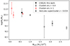 |
Fig. 11. Fitted turnover parameter from Eq. (4) for all the clusters in the study as a function of M200. The black-filled and open circles are, from left to right, the clusters at z ∼ 0.4, Cl0024, MACS0416, Cl0939, and RXJ2248, respectively. The open red triangles are, from left to right, the clusters at z > 1, XMM–LSS J02182–05102, PKS 1138–262, and XMMXCS J2215.9–1738. The black star is the Hercules Supercluster at z ∼ 0.033. |
4.3. Effect of the redshift
Figure 12 shows the MZR for clusters at different redshifts: cluster XMMXCS J2215.9–1738, hereafter XCS2215, at z ∼ 1.5 from Maier et al. (2019), cluster XMM–LSS J02182–05102, hereafter LSS2182, at z ∼ 1.62 form Tran et al. (2015), and the cluster PKS 1138–262, hereafter PKS1138, at z ∼ 2.16 from Pérez-Martínez et al. (2023). XCS2215 and PKS1138 have similar values for M200. On the other hand, LSS2182 has a somewhat lower value of M200, but with large uncertainty, (7.7 ± 3.8)×1013 M⊙ (Pierre et al. 2012), and so we can consider that, in this case, we are mainly comparing the effect of the redshift between the three clusters. In order to carry out a meaningful comparison with the high-redshift clusters, which are limited to high-stellar-mass galaxies, we restricted the galaxies of Cl0024 to stellar masses larger than log(M*/M⊙) > 9.5.
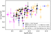 |
Fig. 12. MZR for ELGs in clusters at different redshifts. We show the galaxies from Cl0024 with errors in the determination of the metallicity below 0.3 dex and stellar masses over log(M/M⊙) = 9.5 with filled black circles, the data from Maier et al. (2019) for the cluster XMMXCS J2215.9–1738 at z ∼ 1.5 with blue circles, the data from Tran et al. (2015) for XMM–LSS J02182–05102 at z ∼ 1.62 with magenta circles, and the data from Pérez-Martínez et al. (2023) for the cluster PKS 1138–262 at z ∼ 2.16 with orange circles. |
Figure 13 shows the fit drawn using Eq. (4). All the clusters are approximately superimposed. The fitted values for PKS1138 and Cl0024 are the same within uncertainties. From Table 3, we can see that the values of the turnover mass are also compatible within the uncertainties, as shown in Fig. 11. The only difference between the three clusters is on the γ parameter, which in this case is somewhat higher for XCS2215 when compared with the other clusters.
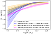 |
Fig. 13. MZR for ELGs in clusters at different redshifts. We show the fitted values from Eq. (4) and the 1σ deviation for the three clusters (filled regions) employing the same colours as in Fig. 12. |
For a fixed stellar mass, Ly et al. (2016) show that the abundance of field galaxies evolves with redshift as log(O/H)∝(1 + z)−2.32. Moreover, Maiolino et al. (2008) found an evolution on the MZR with redshift, and found it to be faster at 2.2 < z < 3.5 than at lower redshifts (z < 2.2). Also Huang et al. (2019) also found that the more evolved galaxies have higher metallicities at fixed stellar masses when compared with less evolved galaxies. Also, Troncoso et al. (2014) found that at z ∼ 3.4, galaxies are more metal poor when compared with lower-redshift galaxies. We do not find a similar relationship with galaxy clusters, although we do not have data over z > 2. This may imply that the effect of the environment, such as the total mass of the cluster, may have a larger influence than the canonical evolution of the cluster.
4.4. Comparison with field galaxies at the same redshift
Figure 14 shows the MZR for our galaxies in Cl0024 and field galaxies at the same redshift from several authors: Amorín et al. (2015), Nadolny et al. (2020), and SDSS field galaxies at 0.35 < z < 0.45 from the Tempel et al. (2017) catalogue, as well as SFGs with 0.35 < z < 0.45 from VIMOS VLT Deep Survey Database (see Le Fèvre et al. 2005 for the description of the survey). From Table 3, we can see that the turnover mass for the field galaxies is the largest one: log(M*/M⊙) = 11.66 ± 0.51 when compared with log(M*/M⊙) = 10.68 ± 0.34 for Cl0024 or log(M*/M⊙) = 9.50 ± 017 for SDSS local clusters. This means that the power-law part of Eq. (4) is dominant for a longer range.
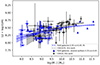 |
Fig. 14. MZR for Cl0024 and field galaxies at similar redshift. Cl0024 galaxies are represented as open grey circles, and field galaxies are represented as filled blue triangles. The field galaxies come from Nadolny et al. (2020), Amorín et al. (2015), and SDSS galaxies at 0.35 < z < 0.45. The fitted value for the MZR is represented by the grey dashed line and the blue dashed line for Cl0024 and field galaxies, respectively. The filled areas represent a 1σ deviation of the fit. |
In this case, for lower stellar masses, the abundance of Cl0024 is compatible with the field galaxies at the same redshift, although the abundance is slightly lower for Cl0024. However, at masses over log(M*/M⊙) > 9.75, the metallicity of the cluster is slightly larger than that of the field galaxies. This seems to agree with the results from Kacprzak et al. (2015), where the authors found no difference larger than 0.02 dex in the MZR of field galaxies at z ∼ 2 when compared with cluster galaxies at the same redshift.
5. Discussion and conclusions
Figure 15 shows all the fits calculated for Eq. (4) for all the clusters presented in this work and field galaxies at z ∼ 0.4 from several sources. We also include data from the Hercules Supercluster, a massive cluster (M200 = 2.1 × 10¹⁵ M⊙ according to Monteiro-Oliveira et al. 2022) at an almost local redshift of z ∼ 0.033. These data were obtained from Petropoulou et al. (2011) for Abell 2151 (the Hercules cluster proper) and from Petropoulou (2012) for the rest of the subclusters that make up the Hercules Supercluster.
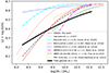 |
Fig. 15. MZR fits for galaxy clusters and field galaxies at z ∼ 0.4. The meaning of the colour code and shape of the lines is explained in the inset key. |
Figure 16 shows the offsets from the fit of the MZR of field galaxies at 0.35 < z < 0.45. It is clear that Cl0024 and MACS0416 clusters both have lower metallicity at lower stellar masses when compared with field galaxies; they also present lower metallicities at all stellar masses when compared with the two more massive clusters Cl0939 and RXJ2248. It should be noted that the two massive clusters RXJ2248 and Cl0939 present a larger value of the turnover parameter M0 when compared with the rest of the clusters. The same also happens at local values of the redshift for the Hercules Supercluster (see Fig. 11).
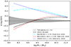 |
Fig. 16. Offsets from the fitted value of MZR of field galaxies at z ∼ 0.4 for clusters at similar redshift. The filled area represents a 1σ deviation of the fit for field galaxies. The colour coding and shape of the lines are explained in the inset key. |
The difference presented in Fig. 16 can be explained if we consider that more massive clusters should present larger zones with high density, where the galaxy–galaxy encounters as well as galaxy–cluster interactions (due to a large virial radius) may be more effective than in smaller clusters. For this reason, low-mass galaxies immersed in massive clusters tend to be more metallic than those in smaller clusters. Therefore, in all these cases, the value of the M0 parameter may be a proxy for the mass of the cluster, and therefore an indicator of the quenching of the star formation in clusters. However, a proper study of the SFR is being carried out (De Daniloff et al., in prep.) to confirm whether or not we are seeing a genuine quenching of the star formation.
Regarding the dynamical state of the cluster, gas metallicity estimations appear not to be affected by the membership of the galaxy to any of the two identified structures confirmed by Sánchez-Portal et al. (2015). So far, we can simply conclude that such structural duality only appears to affect density indicators, in the sense that the median projected surface density (Σ10) of Structure A is ∼0.7 dex denser than that of Structure B (see Sect. 3).
On the other hand, as seen in Figs. 14 and 16, the less massive clusters (Cl0024 and MACS0416) present values for MZR closer to those of field galaxies at the same redshift, with differences in abundance at lower masses of about −0.15 dex and 0.1 dex when compared to the more massive galaxies. This seems to indicate that the conditions in these clusters are much closer to those of field galaxies than to those of more massive clusters.
The main conclusions we can derive from this work are as follows:
-
We revisited the work of Sánchez-Portal et al. (2015) and applied the inverse convolution method to the galaxy cluster Cl0024. We obtain a total of 84 galaxies (classified in tiers 1 to 3) from the original 174, where the method yields better results in the determination of the fluxes and redshifts, and we are able to reduce the uncertainties from over 20% in the old catalogue to less than 10% for the 40% of ELGs, and even below 5% for the 20% of the ELGs.
-
From the redshift distribution, we find the two clearly differentiated structures previously mentioned in Czoske et al. (2002) and Moran et al. (2007), as well as the third interacting structure at about z ∼ 0.42 suggested in Sánchez-Portal et al. (2015).
-
There is a relationship between the clustercentric radius and the logarithm of the density, with galaxies with larger radii being located in zones with lower density when compared with galaxies in the central zones. This effect happens for the two main structures. This seems to imply that both structures may have their nucleus in the line of sight, and therefore may be superimposed.
-
We obtain the MZR for the ELGs of Cl0024 after removing AGNs, indicated as such in Sánchez-Portal et al. (2015).
-
We fitted Cl0024 MZR with the function proposed by Curti et al. (2020), as well as several other clusters and field galaxies.
-
The MZR for Cl0024 presents a tight correlation between the metallicity and the stellar mass of the galaxies, with galaxies with higher masses having higher values of oxygen abundance.
-
We separated the galaxies of Structures A and B in the MZR of Cl0024, as well as the galaxies in high-density zones and low-density zones, and find no differences between them. These results agree with Sobral et al. (2016), where we find no significant dependence of the MZR on the environment inside the same cluster.
-
We find a slight gradient of the metallicity with the clustercentric radius for galaxies of Structure A. Galaxies tend to be more metallic in the inner part of the cluster when compared with galaxies on the outskirts.
-
We find a difference in MZRs for galaxy clusters at the same redshift. Cl0939 and RXJ2248 data from Sobral et al. (2016) and Ciocan et al. (2020), respectively, present larger values of abundance up to stellar masses over log(M*/M⊙) > 10.5. This difference seems to depend on the M200 of each cluster, in the sense that clusters with larger masses have lower values of the turnover mass, M0. This is the case even if the intracluster gas abundance is similar for the clusters. However, the clusters Cl0939 and RXJ2248 present high-density zones with larger values of intracluster gas abundance when compared with Cl0024 and MACS0416. This may imply that the more massive clusters present more galaxy–galaxy as well as cluster–galaxy encounters, which may cause a quenching of the star-forming processes.
-
No appreciable difference was found in the MZR of clusters of similar or lower M200 but different redshift than Cl0024. This seems to suggest that the way in which clusters evolve is heavily influenced by the total mass of the cluster.
-
When comparing Cl0024 with field galaxies at the same redshift, it we find that the MZR fit of field galaxies presents a larger turnover mass, although there is little difference in the abundance of lower stellar masses.
Acknowledgments
B.C., M.S.P., and A.B. acknowledge the support of the Spanish Ministry of Science, Innovation and Universities through the project PID-2021-122544NB-C43. J.C. and M.G.-O. acknowledges the support of the Spanish Ministry of Science, Innovation and Universities through the project PID-2021-122544NB-C41. M.A.L.L. acknowledges support from the Spanish grant PID-2021-123417OB-I00, and the Ramón y Cajal program funded by the Spanish Government (RYC2020-029354-I). M.C. acknowledges the support of PID2019-107408GB-C41 and PID2022-136598NB-C33 grants funded by MCIN/AEI/10.13039/501100011033 and by “ERDF A way of making Europe”. B.C. wishes to thank Carlota Leal Álvarez by her support during the development of this paper. Based on observations made with the Gran Telescopio Canarias (GTC), installed at the Spanish Observatorio del Roque de los Muchachos of the Instituto de Astrofísica de Canarias, on the island of La Palma. This research uses data from the VI-MOSS VLT Deep Survey, obtained from the VVDS database operated by Cesam Laboratoire d’Astrophysique de Marseille, France. This research has made use of NASA’s Astrophysics Data System. This research has made use of the NASA/IPAC Extragalactic Database (NED), which is funded by the National Aeronautics and Space Administration and operated by the California Institute of Technology.
References
- Allen, R. J., Kacprzak, G. G., Glazebrook, K., et al. 2016, ApJ, 826, 60 [Google Scholar]
- Amorín, R., Pérez-Montero, E., Contini, T., et al. 2015, A&A, 578, A105 [NASA ADS] [CrossRef] [EDP Sciences] [Google Scholar]
- Andrews, B. H., & Martini, P. 2013, ApJ, 765, 140 [NASA ADS] [CrossRef] [Google Scholar]
- Arnouts, S., Cristiani, S., Moscardini, L., et al. 1999, MNRAS, 310, 540 [Google Scholar]
- Balogh, M. L., Morris, S. L., Yee, H. K. C., Carlberg, R. G., & Ellingson, E. 1997, ApJ, 488, L75 [NASA ADS] [CrossRef] [Google Scholar]
- Beyoro-Amado, Z., Sánchez-Portal, M., Bongiovanni, Á., et al. 2021, MNRAS, 501, 2430 [CrossRef] [Google Scholar]
- Bonamigo, M., Grillo, C., Ettori, S., et al. 2017, ApJ, 842, 132 [NASA ADS] [CrossRef] [Google Scholar]
- Bonamigo, M., Grillo, C., Ettori, S., et al. 2018, ApJ, 864, 98 [Google Scholar]
- Bongiovanni, Á., Ramón-Pérez, M., Pérez García, A. M., et al. 2019, A&A, 631, A9 [NASA ADS] [CrossRef] [EDP Sciences] [Google Scholar]
- Bongiovanni, Á., Ramón-Pérez, M., Pérez García, A. M., et al. 2020, A&A, 635, A35 [NASA ADS] [CrossRef] [EDP Sciences] [Google Scholar]
- Boselli, A., & Gavazzi, G. 2006, PASP, 118, 517 [Google Scholar]
- Bruzual, G., & Charlot, S. 2003, MNRAS, 344, 1000 [NASA ADS] [CrossRef] [Google Scholar]
- Butcher, H., & Oemler, A. 1978, ApJ, 219, 18 [NASA ADS] [CrossRef] [Google Scholar]
- Calabrò, A., Amorín, R., Fontana, A., et al. 2017, A&A, 601, A95 [NASA ADS] [CrossRef] [EDP Sciences] [Google Scholar]
- Calzetti, D., Armus, L., Bohlin, R. C., et al. 2000, ApJ, 533, 682 [NASA ADS] [CrossRef] [Google Scholar]
- Cantale, N., Jablonka, P., Courbin, F., et al. 2016, A&A, 589, A82 [NASA ADS] [CrossRef] [EDP Sciences] [Google Scholar]
- Cedrés, B., Bongiovanni, Á., Cerviño, M., et al. 2021, A&A, 649, A73 [NASA ADS] [CrossRef] [EDP Sciences] [Google Scholar]
- Cepa, J., Bongiovanni, A., Pérez García, A. M., et al. 2013, Rev. Mex. Astron. Astrofis. Conf. Ser., 42, 70 [NASA ADS] [Google Scholar]
- Cerviño, M., & Valls-Gabaud, D. 2003, MNRAS, 338, 481 [CrossRef] [Google Scholar]
- Chabrier, G. 2003, PASP, 115, 763 [Google Scholar]
- Ciocan, B. I., Maier, C., Ziegler, B. L., & Verdugo, M. 2020, A&A, 633, A139 [NASA ADS] [CrossRef] [EDP Sciences] [Google Scholar]
- Cooper, M. C., Tremonti, C. A., Newman, J. A., & Zabludoff, A. I. 2008, MNRAS, 390, 245 [NASA ADS] [CrossRef] [Google Scholar]
- Cucciati, O., Marinoni, C., Iovino, A., et al. 2010, A&A, 520, A42 [NASA ADS] [CrossRef] [EDP Sciences] [Google Scholar]
- Curti, M., Mannucci, F., Cresci, G., & Maiolino, R. 2020, MNRAS, 491, 944 [Google Scholar]
- Czoske, O., Moore, B., Kneib, J. P., & Soucail, G. 2002, A&A, 386, 31 [NASA ADS] [CrossRef] [EDP Sciences] [Google Scholar]
- Darvish, B., Mobasher, B., Sobral, D., et al. 2015, ApJ, 814, 84 [NASA ADS] [CrossRef] [Google Scholar]
- De Filippis, E., Schindler, S., & Castillo-Morales, A. 2003, A&A, 404, 63 [NASA ADS] [CrossRef] [EDP Sciences] [Google Scholar]
- Dressler, A. 1980, ApJ, 236, 351 [Google Scholar]
- Dressler, A., Thompson, I. B., & Shectman, S. A. 1985, ApJ, 288, 481 [NASA ADS] [CrossRef] [Google Scholar]
- Ellison, S. L., Simard, L., Cowan, N. B., et al. 2009, MNRAS, 396, 1257 [NASA ADS] [CrossRef] [Google Scholar]
- Gisler, G. R. 1978, MNRAS, 183, 633 [NASA ADS] [CrossRef] [Google Scholar]
- Gunn, J. E., & Gott, J. R., III 1972, ApJ, 176, 1 [Google Scholar]
- Hayashi, M., Motohara, K., Shimasaku, K., et al. 2009, ApJ, 691, 140 [NASA ADS] [CrossRef] [Google Scholar]
- Huang, C., Zou, H., Kong, X., et al. 2019, ApJ, 886, 31 [NASA ADS] [CrossRef] [Google Scholar]
- Ilbert, O., Arnouts, S., McCracken, H. J., et al. 2006, A&A, 457, 841 [NASA ADS] [CrossRef] [EDP Sciences] [Google Scholar]
- Johnson, H. L., Harrison, C. M., Swinbank, A. M., et al. 2016, MNRAS, 460, 1059 [NASA ADS] [CrossRef] [Google Scholar]
- Kacprzak, G. G., Yuan, T., Nanayakkara, T., et al. 2015, ApJ, 802, L26 [NASA ADS] [CrossRef] [Google Scholar]
- Kesebonye, K. C., Hilton, M., Knowles, K., et al. 2023, MNRAS, 518, 3004 [Google Scholar]
- Koyama, Y., Kodama, T., Nakata, F., Shimasaku, K., & Okamura, S. 2011, ApJ, 734, 66 [NASA ADS] [CrossRef] [Google Scholar]
- Lara-López, M. A., Cepa, J., Bongiovanni, A., et al. 2010, A&A, 521, L53 [CrossRef] [EDP Sciences] [Google Scholar]
- Lara-López, M. A., Galán-de Anta, P. M., Sarzi, M., et al. 2022, A&A, 660, A105 [NASA ADS] [CrossRef] [EDP Sciences] [Google Scholar]
- Larson, R. B., Tinsley, B. M., & Caldwell, C. N. 1980, ApJ, 237, 692 [Google Scholar]
- Le Fèvre, O., Vettolani, G., Garilli, B., et al. 2005, A&A, 439, 845 [Google Scholar]
- Lee, H., Skillman, E. D., Cannon, J. M., et al. 2006, ApJ, 647, 970 [NASA ADS] [CrossRef] [Google Scholar]
- Ly, C., Malkan, M. A., Rigby, J. R., & Nagao, T. 2016, ApJ, 828, 67 [NASA ADS] [CrossRef] [Google Scholar]
- Maier, C., Ziegler, B. L., Lilly, S. J., et al. 2015, A&A, 577, A14 [NASA ADS] [CrossRef] [EDP Sciences] [Google Scholar]
- Maier, C., Kuchner, U., Ziegler, B. L., et al. 2016, A&A, 590, A108 [NASA ADS] [CrossRef] [EDP Sciences] [Google Scholar]
- Maier, C., Hayashi, M., Ziegler, B. L., & Kodama, T. 2019, A&A, 626, A14 [NASA ADS] [CrossRef] [EDP Sciences] [Google Scholar]
- Maiolino, R., Nagao, T., Grazian, A., et al. 2008, A&A, 488, 463 [NASA ADS] [CrossRef] [EDP Sciences] [Google Scholar]
- Mann, A. W., & Ebeling, H. 2012, MNRAS, 420, 2120 [NASA ADS] [CrossRef] [Google Scholar]
- Marino, R. A., Rosales-Ortega, F. F., Sánchez, S. F., et al. 2013, A&A, 559, A114 [NASA ADS] [CrossRef] [EDP Sciences] [Google Scholar]
- Monteiro-Oliveira, R., Morell, D. F., Sampaio, V. M., Ribeiro, A. L. B., & de Carvalho, R. R. 2022, MNRAS, 509, 3470 [Google Scholar]
- Moore, B., Katz, N., Lake, G., Dressler, A., & Oemler, A. 1996, Nature, 379, 613 [Google Scholar]
- Moran, S. M., Ellis, R. S., Treu, T., et al. 2005, ApJ, 634, 977 [NASA ADS] [CrossRef] [Google Scholar]
- Moran, S. M., Ellis, R. S., Treu, T., et al. 2007, ApJ, 671, 1503 [Google Scholar]
- Mouhcine, M., Baldry, I. K., & Bamford, S. P. 2007, MNRAS, 382, 801 [NASA ADS] [CrossRef] [Google Scholar]
- Moustakas, J., Zaritsky, D., Brown, M., et al. 2011, ArXiv e-prints [arXiv:1112.3300] [Google Scholar]
- Nadolny, J., Lara-López, M. A., Cerviño, M., et al. 2020, A&A, 636, A84 [NASA ADS] [CrossRef] [EDP Sciences] [Google Scholar]
- Navarro Martínez, R., Pérez-García, A. M., Pérez-Martínez, R., et al. 2021, A&A, 653, A24 [NASA ADS] [CrossRef] [EDP Sciences] [Google Scholar]
- Old, L. J., Balogh, M. L., van der Burg, R. F. J., et al. 2020, MNRAS, 493, 5987 [NASA ADS] [CrossRef] [Google Scholar]
- Pérez-Martínez, J. M., Dannerbauer, H., Kodama, T., et al. 2023, MNRAS, 518, 1707 [Google Scholar]
- Petropoulou, V. 2012, PhD Thesis, University of Granada, Spain [Google Scholar]
- Petropoulou, V., Vílchez, J., Iglesias-Páramo, J., et al. 2011, ApJ, 734, 32 [NASA ADS] [CrossRef] [Google Scholar]
- Pettini, M., & Pagel, B. E. J. 2004, MNRAS, 348, L59 [NASA ADS] [CrossRef] [Google Scholar]
- Pierre, M., Clerc, N., Maughan, B., et al. 2012, A&A, 540, A4 [NASA ADS] [CrossRef] [EDP Sciences] [Google Scholar]
- Rahaman, M., Raja, R., Datta, A., et al. 2021, MNRAS, 505, 480 [NASA ADS] [CrossRef] [Google Scholar]
- Sánchez-Portal, M., Pintos-Castro, I., Pérez-Martínez, R., et al. 2015, A&A, 578, A30 [NASA ADS] [CrossRef] [EDP Sciences] [Google Scholar]
- Schindler, S., Belloni, P., Ikebe, Y., et al. 1998, A&A, 338, 843 [NASA ADS] [Google Scholar]
- Shimakawa, R., Kodama, T., Tadaki, K. I., et al. 2014, MNRAS, 441, L1 [NASA ADS] [CrossRef] [Google Scholar]
- Sobral, D., Stroe, A., Koyama, Y., et al. 2016, MNRAS, 458, 3443 [NASA ADS] [CrossRef] [Google Scholar]
- Tempel, E., Tuvikene, T., Kipper, R., & Libeskind, N. I. 2017, A&A, 602, A100 [NASA ADS] [CrossRef] [EDP Sciences] [Google Scholar]
- Tran, K.-V. H., Nanayakkara, T., Yuan, T., et al. 2015, ApJ, 811, 28 [NASA ADS] [CrossRef] [Google Scholar]
- Tremonti, C. A., Heckman, T. M., Kauffmann, G., et al. 2004, ApJ, 613, 898 [Google Scholar]
- Troncoso, P., Maiolino, R., Sommariva, V., et al. 2014, A&A, 563, A58 [NASA ADS] [CrossRef] [EDP Sciences] [Google Scholar]
- Vaughan, S. P., Tiley, A. L., Davies, R. L., et al. 2020, MNRAS, 496, 3841 [NASA ADS] [CrossRef] [Google Scholar]
- Zahid, H. J., Dima, G. I., Kudritzki, R.-P., et al. 2014, ApJ, 791, 130 [NASA ADS] [CrossRef] [Google Scholar]
- Zhang, Y. Y., Böhringer, H., Mellier, Y., Soucail, G., & Forman, W. 2005, A&A, 429, 85 [NASA ADS] [CrossRef] [EDP Sciences] [Google Scholar]
Appendix A: List of galaxies from tiers 1 to 3
Catalogue of deconvolved galaxies with quality tiers 1 to 3. The first column is the identification number from Sánchez-Portal et al. (2015); column 2 is the new derived redshift; column 3 and 4 are the integrated Hα flux and [N II]λ6583, respectively, in erg cm−2 s−1 × 10⁻¹⁷; column 5 is the derived abundance employing the N2 index; column 6 is the logarithm of the stellar mass in solar masses, and column 7 is the flag for AGN from Sánchez-Portal et al. (2015). The uncertainties are taken as one standard deviation of the value of each parameter.
All Tables
Catalogue of deconvolved galaxies with quality tiers 1 to 3. The first column is the identification number from Sánchez-Portal et al. (2015); column 2 is the new derived redshift; column 3 and 4 are the integrated Hα flux and [N II]λ6583, respectively, in erg cm−2 s−1 × 10⁻¹⁷; column 5 is the derived abundance employing the N2 index; column 6 is the logarithm of the stellar mass in solar masses, and column 7 is the flag for AGN from Sánchez-Portal et al. (2015). The uncertainties are taken as one standard deviation of the value of each parameter.
All Figures
|
Fig. 1. Pseudospectrum with fitting components (upper panel) and deconvolved spectrum (lower panel) for the tier 1 galaxy id:424. The filled grey area represents the 68% confidence interval. |
| In the text | |
|
Fig. 2. Redshift distribution for the galaxies presented in this study of Cl0024. The upper panel shows the distribution of redshifts derived from the new determination (solid line) and the determination from Sánchez-Portal et al. (2015) (dashed line). The lower panel shows the distribution of the residuals between the old and the new redshift determination. This figure includes all the galaxies (tiers 1 to 3, and “no deblending” and “composite Hα, lines”). |
| In the text | |
|
Fig. 3. Comparison between the obtained values for the Hα emission line uncorrected for extinction from Sánchez-Portal et al. (2015) and the new one from this work. The red continuous line indicates a 1:1 relation. |
| In the text | |
|
Fig. 4. Histogram of the relative uncertainty in the flux determination in the Hα line. The red histogram is the error from Sánchez-Portal et al. (2015). The red dotted line is the median value of the relative error. The black histogram is the relative error from this work. The grey dashed line represents the median value. |
| In the text | |
|
Fig. 5. Logarithm of Σ10 as a function of the clustercentric radius for all the galaxies from Sánchez-Portal et al. (2015). Open circles and downward-pointing filled triangles are the galaxies from Structures A and B, respectively. The grey and red dashed lines show the median value for galaxies in Structures A and B, respectively. The filled grey and red areas represent the median absolute deviation for Structures A and B, respectively. |
| In the text | |
|
Fig. 6. MZR for the SFGs of Cl0024. Our data are the open circles, the black-dashed line represents the mean of the fitted values employing the recipe by Curti et al. (2020), and the grey area represents the 1σ deviation of the fits. |
| In the text | |
|
Fig. 7. MZR for Cl0024. Left panel: open black circles and red filled circles are the galaxies with R < 0.5 R200 and galaxies in Structure B, respectively. Right panel: open red circles and open black circles are the galaxies from Cl0024 within medium and high-density zones (log(Σ10)≧1.7) and low-density zones (log(Σ10) < 1.7), respectively. |
| In the text | |
|
Fig. 8. Metallicity as a function of clustercentric radius for Cl0024. The open black circles are the galaxies from Structure A. The downward black-filled triangles are the galaxies from Structure B. The grey dashed line is the median of the values for Structure A. The blue dotted line indicates the position of the virial radius for Cl0024 from Sánchez-Portal et al. (2015). |
| In the text | |
|
Fig. 9. Mass–metallicity relationship for ELGs in clusters at similar redshift. Black circles represent our data. The cyan downward-pointing triangles are the galaxies from Ciocan et al. (2020) for the cluster RX J2248–4431. The blue pentagons represent the galaxies from Sobral et al. (2016) for the cluster Cl 0939+4713. The red upward-pointing triangles are the galaxies from Maier et al. (2016) for the cluster MACS J0416.1–2403. |
| In the text | |
|
Fig. 10. Comparison of MZR between Cl0024 and clusters at the same redshift, as well as galaxies from clusters at low redshift from Tempel et al. (2017). The colour coding is reported in the legend. All data were fitted following the recipe presented in Curti et al. (2020). |
| In the text | |
|
Fig. 11. Fitted turnover parameter from Eq. (4) for all the clusters in the study as a function of M200. The black-filled and open circles are, from left to right, the clusters at z ∼ 0.4, Cl0024, MACS0416, Cl0939, and RXJ2248, respectively. The open red triangles are, from left to right, the clusters at z > 1, XMM–LSS J02182–05102, PKS 1138–262, and XMMXCS J2215.9–1738. The black star is the Hercules Supercluster at z ∼ 0.033. |
| In the text | |
|
Fig. 12. MZR for ELGs in clusters at different redshifts. We show the galaxies from Cl0024 with errors in the determination of the metallicity below 0.3 dex and stellar masses over log(M/M⊙) = 9.5 with filled black circles, the data from Maier et al. (2019) for the cluster XMMXCS J2215.9–1738 at z ∼ 1.5 with blue circles, the data from Tran et al. (2015) for XMM–LSS J02182–05102 at z ∼ 1.62 with magenta circles, and the data from Pérez-Martínez et al. (2023) for the cluster PKS 1138–262 at z ∼ 2.16 with orange circles. |
| In the text | |
|
Fig. 13. MZR for ELGs in clusters at different redshifts. We show the fitted values from Eq. (4) and the 1σ deviation for the three clusters (filled regions) employing the same colours as in Fig. 12. |
| In the text | |
|
Fig. 14. MZR for Cl0024 and field galaxies at similar redshift. Cl0024 galaxies are represented as open grey circles, and field galaxies are represented as filled blue triangles. The field galaxies come from Nadolny et al. (2020), Amorín et al. (2015), and SDSS galaxies at 0.35 < z < 0.45. The fitted value for the MZR is represented by the grey dashed line and the blue dashed line for Cl0024 and field galaxies, respectively. The filled areas represent a 1σ deviation of the fit. |
| In the text | |
|
Fig. 15. MZR fits for galaxy clusters and field galaxies at z ∼ 0.4. The meaning of the colour code and shape of the lines is explained in the inset key. |
| In the text | |
|
Fig. 16. Offsets from the fitted value of MZR of field galaxies at z ∼ 0.4 for clusters at similar redshift. The filled area represents a 1σ deviation of the fit for field galaxies. The colour coding and shape of the lines are explained in the inset key. |
| In the text | |
Current usage metrics show cumulative count of Article Views (full-text article views including HTML views, PDF and ePub downloads, according to the available data) and Abstracts Views on Vision4Press platform.
Data correspond to usage on the plateform after 2015. The current usage metrics is available 48-96 hours after online publication and is updated daily on week days.
Initial download of the metrics may take a while.