| Issue |
A&A
Volume 686, June 2024
|
|
|---|---|---|
| Article Number | A224 | |
| Number of page(s) | 8 | |
| Section | The Sun and the Heliosphere | |
| DOI | https://doi.org/10.1051/0004-6361/202348606 | |
| Published online | 14 June 2024 | |
Long-period oscillations in the lower solar atmosphere prior to flare events
1
Leibniz-Institut für Astrophysik Potsdam (AIP), An der Sternwarte 16, 14-482 Potsdam, Germany
e-mail: This email address is being protected from spambots. You need JavaScript enabled to view it.
2
Dipartimento di Fisica e Astronomia “Ettore Majorana”, Università di, Catania, Via S. Sofia 78, 95123 Catania, Italy
3
Department of Astronomy, Eötvös Loránd University, Pázmány Péter sétány 1/A, 1112 Budapest, Hungary
4
Solar Physics and Space Plasma Research Center, School of Mathematics and Statistics, University of Sheffield, Sheffield S3 7RH, UK
5
Hungarian Solar Physics Foundation, Petőfi tér 3, 5700 Gyula, Hungary
Received:
14
November
2023
Accepted:
11
March
2024
Abstract
Context. Multiple studies have identified a range of oscillation periods in active regions, from 3−5 min to long-period oscillations that last from tens of minutes to several hours. Recently, it was also suggested that these periods are connected with eruptive activity in the active regions. Thus, it is essential to understand the relation between oscillations in solar active regions and their solar eruption activity.
Aims. We investigate the long-period oscillations of NOAA 12353 prior to a series of C-class flares and correlate the findings with the 3- to 5-min oscillations that were previously studied in the same active region. The objective of this work is to elucidate the presence of various oscillations with long periods in the lower solar atmosphere both before and after the flare events.
Methods. To detect long-period oscillations, we assessed the emergence, shearing, and total magnetic helicity flux components from the photosphere to the top of the chromosphere. To analyze the magnetic helicity flux in the lower solar atmosphere, we used linear force-free field extrapolation to construct a model of the magnetic field structure of the active region. Subsequently, the location of long-period oscillations in the active region was probed by examining the spectral energy density of the measured intensity signal in the 1700 Å, 1600 Å, and 304 Å channels of the Atmospheric Imaging Assembly (AIA) of the Solar Dynamics Observatory (SDO). Significant oscillation periods were determined by means of a wavelet analysis.
Results. Based on the evolution of the three magnetic helicity flux components, 3- to 8-h periods were found both before and after the flare events, spanning from the photosphere to the chromosphere. These 3- to 8-h periods were also evident throughout the active region in the photosphere in the 1700 Å channel. Observations of AIA 1600 Å and 304 Å channels, which cover the chromosphere to the transition region, revealed oscillations of 3−8 h near the region in which the flare occurred. The spatial distribution of the measured long-period oscillations mirror the previously reported distribution of 3- to 5-min oscillations in NOAA 12353 that were seen both before and after the flares.
Conclusions. This case study suggest that the varying oscillation properties in a solar active region could be indicative of future flaring activity.
Key words: magnetohydrodynamics (MHD) / waves / Sun: flares / Sun: magnetic fields / Sun: oscillations / Sun: photosphere
© The Authors 2024
 Open Access article, published by EDP Sciences, under the terms of the Creative Commons Attribution License (https://creativecommons.org/licenses/by/4.0), which permits unrestricted use, distribution, and reproduction in any medium, provided the original work is properly cited.
This article is published in open access under the Subscribe to Open model. This email address is being protected from spambots. You need JavaScript enabled to view it. to support open access publication.
1. Introduction
Active regions (ARs) represent zones with intense magnetic fields that can be observed on the solar surface and in the lower solar atmosphere. ARs play a significant role in solar events, including solar flares and coronal mass ejections (CME). Detailed, high-resolution observations highlight the intricate structures and dynamic behaviors of ARs. These regions, along with the sunspots they encompass, notably display a diverse range of waves and oscillations.
The oscillatory behaviors in ARs can be classified into several categories. The more commonly recognized categories are short-period oscillations with a typical duration of 3 (Fleck & Schmitz 1991) and 5 (Thomas et al. 1984) minutes. Other detected periods include long-period oscillations spanning several hours (see Efremov et al. 2007; Dorotovič et al. 2008, 2014; Dumbadze et al. 2017, and references therein), and the ultra-long-period oscillations that persist for days (see Khutsishvili et al. 1998; Gopasyuk 2004, and references therein).
Bhatnagar et al. (1972) was one of the first to document this 5-min short-period oscillation in photospheric umbral fluctuations. These 5-min oscillations within a sunspot umbra are a testament to how a sunspot may react to the surrounding 5-min p-modes in the ambient calm regions (as discussed in Thomas et al. 1982, and the references therein). Interestingly, in the elevated atmosphere over sunspot umbrae (Ruiz Cobo et al. 1997), 3-min oscillations stand out as the dominant dynamic phenomena. These fluctuations are discernible through various chromospheric spectral lines, including the Ca II H and K lines (Beckers & Tallant 1969), Hα (Giovanelli 1972), the Ca II IR triplet (Lites et al. 1982), and the Mg II h and k lines (Gurman 1987). These variations point to a comprehensive wave propagation mechanism within sunspots (Khomenko & Collados 2015; Stangalini et al. 2018). Reinforcing this concept, a plethora of studies have underscored evidence of these wave motions that span from the photosphere to the corona (e.g. Freij et al. 2014; Krishna Prasad et al. 2015; Zhao et al. 2016; Stangalini et al. 2021).
A fundamental observation in the atmosphere of umbrae is the vertical shift in the oscillation period, transitioning from 5-min oscillations in the photosphere to 3-min oscillations in the chromosphere (Beckers & Schultz 1972; Lites 1992). Wiśniewska et al. (2016) also confirmed that since the cutoff frequency in the quiet-Sun region depends on the height, this maximum can also be achieved at frequencies up to 7.0 mHz in the chromosphere, which corresponds to ∼2−3 min. Furthermore, Monsue et al. (2016) examined waves with frequencies (ν) ranging from 0 to 8.0 mHz using the Hα line. Their results showed a power enhancement for frequencies of 1−2 mHz immediately prior to and shortly after the flare. The other frequencies up to 8 mHz were suppressed. Their explanation for this behavior was that acoustic energy is converted into thermal energy at the flare maximum, while the low-frequency enhancement arose from an instability in the chromosphere and provided an early warning of the flare onset.
Recently, Wiśniewska et al. (2019) analyzed the frequency distribution of short-period oscillations (3 and 5 min) in the lower solar atmosphere before and during a C-class flare event. Interestingly, they found that the location of the enhanced oscillatory power in the 6−7 mHz range (approximately 2.5 min) was initially concentrated around the active region in the photosphere. Meanwhile, these shorter periods were measured precisely in the area of maximum flare emission in the chromosphere, unlike the surrounding area, which did not show the increment of spatial power distribution. Wiśniewska et al. (2019) also applied the differential emission measure (DEM) analysis for this particular region that exhibited rapid oscillatory motions of plasma, heated up to 12 MK inside the magnetic arch, which afterward formed post-flare loops. In the footpoints of the associated chromospheric loop, the temperatures varied from 0.4 MK to 1.0 MK. Therefore, the authors concluded that this phenomenon agreed with the results that were presented by Monsue et al. (2016). These two works support and confirm the conjecture that the energy of the high-frequency waves due to a flare can be converted into thermal energy and transported toward higher layers of the solar atmosphere.
Furthermore, long-period oscillations in sunspots were discerned both from radio emission measurements and magnetic field data, as highlighted by the research of Gelfreikh et al. (2006), Solov’ev & Kirichek (2008), Abramov-Maximov et al. (2013), Smirnova et al. (2013). To date, magnetic field oscillations with periods of 30−40, 70−100, 150−200, and 800−1300 min were observed in ARs by various researchers, for instance, Nagovitsyna & Nagovitsyn (2002), Efremov et al. (2007), Dorotovič et al. (2008, 2014), Kallunki & Riehokainen (2012), Abramov-Maximov et al. (2013), Bakunina et al. (2013), Efremov et al. (2014). Based on the findings of Dumbadze et al. (2021), these long-period oscillations necessitate the energetic backing of convective activities beneath the solar facade. One plausible explanation could be rooted in the diverse magnetohydrodynamic oscillations evident in the stratified structure of the AR magnetic field. These might be intrinsically connected to the characteristic turnover duration of supergranulation cells. Moreover, oscillations detected in radial magnetic flux data might also be indicative of recurring flux emergence or cancellation. It was also suggested by Solov’ev & Kirichek (2008, 2009, 2014), however, that long-period oscillations represent the global vertical-radial oscillations of a magnetic element, such as a spot or pore. These oscillations occur around its stable equilibrium position. These oscillations are indicative of emergence and formation processes of the flux tube forming sunspots. They also symbolize deviations from the gas-mass equilibrium within the sunspot Wilson depression area.
Soós et al. (2022) and Korsós et al. (2022) reported long-period oscillations in the evolution of the magnetic helicity flux preceding solar eruptions. Soós et al. (2022) examined the presence of long-period oscillations in the evolution of the magnetic helicity flux in various flare-producing ARs. They identified and highlighted a correlation between the flaring activities and the unique oscillatory behavior pattern of the horizontal and vertical magnetic helicity flux components. This work was further developed by Korsós et al. (2022). They found that the longest photospheric periods of the horizontal and vertical helicity fluxes remained the longest and most common periods at least up to 1 Mm or even higher days before the most energetic flare events. They concluded that the horizontal and vertical helicity flux components become a coupled oscillatory system in the lower solar atmosphere before a major solar eruption.
Therefore, the aim of this study is to scrutinize in a more systematic manner the presence of long-period oscillations in an AR within the lower solar atmosphere prior to solar eruptions. The active region selected for this study, NOAA 12353, was previously examined by Wiśniewska et al. (2019). The authors primarily focused on the relation between the 3- and 5-min short-period oscillations and the flare activity. Our current investigation specifically targets the relation between the long-period oscillations and the flare activity of this active region, building upon the works of Wiśniewska et al. (2019) and Korsós et al. (2022).
The structure of this paper is as follows: Section 2 offers an introduction to the studied AR, NOAA 12353. Section 3.1 analyzes the magnetic helicity evolution in the lower solar atmosphere. Section 3.2 presents an in-depth analysis of intensity images at the 1700 Å, 1600 Å, and 304 Å wavelengths. Finally, the results and conclusions are presented in Sect. 4.
2. Observational data
The aim of this study is to identify long-period oscillatory patterns in active region NOAA 12353 and investigate the relation of these patterns to its flaring activity. Therefore, we analyzed the corresponding 1700, 1600, and 304 Å observations taken by the Atmospheric Imaging Assembly (AIA; Lemen et al. 2012) camera and magnetic field measurements taken by the Helioseismic and Magnetic Imager (HMI; Schou et al. 2012; Scherrer et al. 2012) on board the Solar Dynamics Observatory (SDO; Pesnell et al. 2012).
The studied AR emerged on 2015 May 21 and was designated NOAA 12353 on the subsequent day. The data sets contain measurements between 2015 May 21 at 17:30 UT and 2015 May 23 at 23:42 UT. On 2015 May 23, a negative magnetic field appeared within two positive polarities. This area of NOAA 12353 is emphasized with the large white squares in Figs. 1a–c. Furthermore, a small opposite-polarity pair was present, which is shown in the smaller white square in Fig. 1a. These close-by opposite magnetic field elements together triggered a series of C-class flares on 2015 May 23: with peak flaring activities of C1.0 flare at 03:33, C1.1 at 07:22, and C2.3 at 17:39 UT. The positive polarity of the small opposite magnetic field pair (in the smaller white square of Fig. 1a) disappeared after the first C1.0 flare, while the larger negative polarity slowly started to disappear close to the end of the study period. After the last C2.3 flare, the AR exhibited a more simplified and matured magnetic structure.
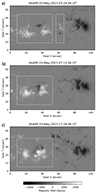 |
Fig. 1. AR NOAA 12353. The panels display the SHARP radial magnetic field component (Br). Panels a–c show the closest magnetogram in time to the X-ray flux peak of C1.0, C1.1, and C2.3, respectively, on 2015 May 23. The larger white square emphasizes the delta spot of the active region. The smaller white square in panel a marks the two close opposite polarities where the positive polarity disappeared after the C1.0 flare. The color bar gives information about the magnetic field strength. |
Similar to Korsós et al. (2022), we employed the linear force-free field (LFFF) extrapolation model as presented by Wiegelmann & Sakurai (2021) to investigate the oscillations of the magnetic helicity flux in the 3D lower solar atmosphere of NOAA 12353. This model hinges on the photospheric vector magnetic field observations. The photospheric vector magnetic fields of the AR comprise the Br, Bt, and Bp components, as sourced from the Spaceweather Helioseismic Magnetic Imager Active Region Patches (SHARPs; Bobra et al. 2014). Using the method developed by Wiegelmann & Sakurai (2021), we constructed a series of extrapolated magnetogram data from the z = 0 level (denoting the photosphere) up to 3.6 Mm with a 12-min cadence. A step size of z = 0.36 Mm was adopted, congruent with the SHARP pixel dimension. Additionally, for the LFFF extrapolation, we leveraged the precalculated and archived twisting parameter α embedded in the FITS header of the SHARP data cube series.
Next, we used the measurements from the Atmospheric Imaging Assembly/SDO (AIA/SDO; Lemen et al. 2012) to investigate the presence and the location of long-period oscillations within the AR before and during the C-class flares. For this purpose, we selected the intensity filtergrams at wavelengths of 1700 Å, 1600 Å, and 304 Å. These data sets encompass the designated area of NOAA 12353 within the 108 × 54 arcsec2 field of view (FoV; Figs. 2a–c). The comprehensive data set of tracked and normalized intensity images spans from 2015 May 21 at 17:30 UT to 2015 May 23 at 23:42 UT. While filtergrams with a temporal resolution of 12 s are available from AIA, we opted for a 12-min cadence to match the cadence of the SHARP data.
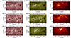 |
Fig. 2. Series of AIA cutouts showing AR NOAA 12353 in panel a in the 1700 Å, in panel b in the 1600 Å, and in panel c in the 304 Å channels. Each row shows a snapshot of the region close to the onset times of C1.0, C1.1, and C2.3 flares. The selected areas have spatial dimensions of 108 × 54 arcsec2, and the axes indicate the position of the region with respect to the solar center. The overplotted black contours represent the largest intensity area during the corresponding flare event measured in the 304 Å wavelength. |
3. Results
3.1. Determining helicity flux oscillations
Magnetic helicity quantifies the extent of twist, writhing, and linkage of magnetic field lines within a given volume (Berger & Field 1984; Berger 1993; Berger & Hornig 2018). It conveys information regarding the intricacy of the magnetic field topology and is therefore associated with the free magnetic energy stored in ARs (Schuck & Antiochos 2019; Liokati et al. 2023). Consequently, specific magnetic helicity parameters are thought to be insightful for characterizing the pre-flare conditions of ARs (e.g., Elsasser 1956; Moon et al. 2002a,b; Smyrli et al. 2010; Park et al. 2008, 2012; Gupta et al. 2021).
Additionally, Korsós et al. (2022) demonstrated that the simultaneous long-period oscillations of the emergence (EM), shearing (SH), and total (T) helicity flux components are discernible from the photosphere up to heights of at least 1 Mm, and can be evident several days preceding a flare event(s).
In alignment with the approach of Korsós et al. (2022), we now computed the magnetic helicity flux to observe its progression, which symbolizes the rate of helicity injection, over various atmospheric layers of the AR. For each scrutinized atmospheric layer of the AR, we employed the technique called differential affine velocity estimator for vector magnetograms (DAVE4VM; Schuck 2008) to ascertain the evolution of the magnetic helicity flux. Following this, to ensure consistency in scale for comparison, we normalized the time series of the three magnetic helicity flux components (EM, SH, and T) using their maximum absolute values.
Next, following the approach and method that were developed and applied, in Korsós et al. (2022) and Soós et al. (2022), we analyzed the time series of the normalized EM (dotted line), SH (solid line), and T (dash-dotted line) helicity flux components, as shown in Fig. 3a. We used the wavelet analysis software developed by Torrence & Compo (1998) to generate the wavelet power spectrum (WPS) of the EM, SH, and T time series using the default Morlet wavelet profile. Furthermore, we calculated the associated global power spectrum (GPS) by averaging the WPS (see, e.g., Fig. 3c). To uncover how the long-period oscillatory behavior of the three helicity flux components develops in the lower solar atmosphere before the flares, we identified significant periodicities based on the GPS and WPS plots with a 2σ significance at each investigated atmospheric height. These measured significant periods at each corresponding height are summarized in Table 1. The 2σ significance levels were determined based on the white-noise model and standard deviation of the input signals.
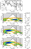 |
Fig. 3. Temporal analysis of the magnetic helicity flux in the photosphere. The top panel a shows time series of the normalized emergence (EM, dotted line), shearing (SH, solid line), and Total (dash-dotted line) helicity fluxes. The vertical black lines mark the onset time of the C1.0 (03:30), C1.1 (07:30), and C2.3 (17:39) flares, respectively, on 2015 May 23. Rows 2–4 (panel b) show the wavelet power spectrum (WPS) of the EM, SH, and Total helicity fluxes. The x-axis of each WPS is the observation time, and the y-axis is the period, both in hours. The black lines in the WPS plots bound the cone of influence (hashed area), i.e., the domain in which edge effects may become important. The plots to the right of each WPS (panel c) are the corresponding global wavelet spectra (GPS) with power averaged over time. The dashed black lines mark the 2σ confidence for GPS analyses. |
Periods of the three magnetic helicity flux components at the investigated heights.
According to Table 1, the revealed periods have two peak oscillation times at 3 and 7 h in the evolution of the EM component from the photosphere up to the chromosphere. Remarkably, these periods persisted both before and after the occurrence of C-class flares. Similarly, the SH and T helicity fluxes exhibit comparable periods, lasting from 3 to 8 h throughout the investigated lower solar atmosphere. However, it is worth noting that the SH and T components also manifest an additional 10-h period, which can be confidently deduced at a 2σ confidence level from the photosphere up to an altitude of 1400 km. The powers of the 10-h period were more dominant during the emerging phase of the AR (see, e.g., Fig. 3). The 3- to 8-h-period band of the three helicity flux components was measurable from the beginning until the end of the investigation period.
3.2. Wavelet analysis of the intensity at 1600 Å, 1700 Å, and 304 Å
The oscillations in the intensity data were studied in two ways. First, we analyzed the time series of the FOV-integrated intensity for each of the three AIA channels (1700 Å, 1600 Å, and 304 Å), and then we analyzed the intensity time series of every pixel of the FOV. The first approach facilitates a direct comparison with the analysis of the helicity, since the FOV-integrated intensity time series characterizes the active region as a whole, and similarly, for the three helicity components. The second approach allows the examination of the spatial distribution of the oscillatory power.
For the first approach, we averaged for each channel the intensity inside the FOV in each filtergram and constructed the time series seen as in the upper panels of Fig. 4. The lower panels of the same figure show the 2D wavelet transform of the series. For the image sequences at 1700 Å and 1600 Å, we could not identify any significant periods (inside the cone of influence that marks the significant results of WPS). However, for the 304 Å data series, we were able to determine significant periods between ∼3 and ∼8 h (see Fig. 4c). The 3-h period, although weaker than the 8-h period, still reaches a 2σ (95%) confidence level. The 8-h period started to be dominant ∼15 h before the first C-class flare. The 3-h period was observed with a 2σ significance around the time of the C1.1 and C1.0 flares.
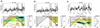 |
Fig. 4. Spatially averaged WPS of the intensity signals for the FoV the NOAA 12353 taken at (a) 1700 Å, (b) 1600 Å, and 304 Å. This figure is to be compared with the results presented in Fig. 3. We identified strong oscillation powers between 3.0−8.0 h for (c) 304 Å. |
Next, for the second approach, we generated 3D wavelet power spectra (wavelet power as a function of time and period) for each pixel within the FoV. We applied the default Morlet wavelet profile to each pixel in the analyzed data cubes. Based on the results of the analysis of the integrated intensity and the helicity parameters, we focused on the 3- to 8-h-period window. Figure 5 represents the 3D data cubes of the spatial distribution of power in the 3- to 8-h-period band as a function of time. In the 3D data cubes, the magnitude of the power increases from green to red.
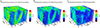 |
Fig. 5. 3D cubes showing the spatial distribution over the FoV of the power in the 3- to 8-h-period band as a function of time in the case of 1700 Å, 1600 Å, and 304 Å, plotted in panels a–c, respectively. |
To pinpoint the 3- to 8-h oscillations within the 3D wavelet power spectra, we took temporal cross cuts through the 3D cubes of Fig. 5 for 1700 Å, 1600 Å, and 304 Å. The cuts were taken at four instances in Figs. 6a–c: (I) before the C1.0 flare on 2015 May 22 at 03:42 UT, (II) about 20 min after the C1.0 flare on 2015 May 23 at 03:54 UT, (III) about 30 min after the C1.1 flare on 2015 May 23 at 07:54 UT, and, finally, (IV) about 15 min after the C2.3 flare on 2015 May 23 at 17:54 UT. From inspecting Figs. 5 and 6, we note the following:
-
In the 1700 Å channel (Fig. 6a), the power of the oscillations with periods between 3 to 8 h appears notably strong around the sunspot at all four selected times. The 1700 Å wavelength predominantly provides insights into the photosphere and temperature minimum region (Lemen et al. 2012). Therefore, the observed 3- to 8-h-period band could be associated with photospheric plasma motions, which in turn may induce magnetic field configurations that support or even trigger solar flares.
-
The 1600 Å channel mostly reflects the evolution of the AR in the upper photosphere and the transition region (Lemen et al. 2012). In Fig. 6b, the highest power of the 3- to 8-h oscillation band is more localized than in Fig. 6a. The power is concentrated in the area in which the opposite polarities are very close to each other, as highlighted in Figs. 1a–c. Furthermore, the regions of high power significantly overlap with the locations of the footpoints of the flaring loop, as shown in Fig. 3.
-
The 304 Å channel shows the evolution of the AR in the chromosphere and transition region (Lemen et al. 2012). Before the occurrence of the first C-class flare, the strongest power outlines the loop structures within the opposite polarities (Fig. 6c). However, during the time when the three flares occurred, the locations of the power peaks are closely aligned with the location of the flares (see Figs. 6c II–IV).
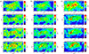 |
Fig. 6. Cuts through the 3D cubes of Fig. 5 for (a) the intensity at 1700 Å, (b) the intensity at 1600 Å, and (c) the intensity at 304 Å, estimated at four moments of time. The panels are (I) before the first flare on 2015 May 22 at 03:42 UT, (II) ∼20 min after the first flare C1.0, (III) ∼30 min after the second flare C1.1, and (IV) ∼15 min after the third flare C2.3. |
As illustrated in Figs. 1 and 6c, NOAA 12353 is an emerging region that produced the three C-class flares during its relatively early stages of evolution. For this region, the 3- to 8-h long-period oscillations were notably strong in the emergence area, particularly within the chromosphere and transition region many hours before the first flare (Figs. 4c and 6c I).
4. Discussion and conclusion
We aimed to merge the methods of Wiśniewska et al. (2019) and Korsós et al. (2022) to examine the presence of long-period oscillations in the lower solar atmosphere in two types of time series. HMI magnetograms were probes of the magnetic complexity, namely the three components of the magnetic helicity, EM, SH, and Total. The others were the observable UV or extreme-UV morphology of the region, namely the intensities recorded by the three AIA channels 1600 Å, 1700 Å, and 304 Å. Both sets of observables stem from a height range spanning from the photosphere up to the upper chromosphere and transition region. We examined the presence of long-period oscillations over a 50-h interval, spanning from the initial emergence phase of NOAA 12353 until the end of its series of three C-class flares. Our goal was to deepen our understanding of the relation between the oscillatory behavior of the AR and flaring activity.
The analysis of the helicity-related time series unveiled dominant periodicities spanning between 3−8 h in the evolution of the EM, SH, and Total components from the photosphere through the chromosphere. Notably, these periods were consistent during the entire investigated period. Additionally, the SH and Total components exhibited an ancillary 10-h period that was confidently ascertained at the 2σ confidence level, from the photosphere to an altitude of approximately 1400 km. These long-period oscillations were particularly pronounced during the emergent phase of the AR.
Interestingly, the oscillatory behavior of the AIA intensities is consistent with these findings. Although the disk-integrated intensity in 1700 Å and 1600 Å does not show any significant signal, the 304 Å shows dominant periods around 3 and 8 h at the 2σ (95%) confidence level. It should be noted that 1700 Å and 1600 Å predominantly reflect the photospheric evolution, with the exception of the latter, which also contains contributions from the chromosphere and transition region C IV line. However, the 304 Å primarily measures He II emission and therefore shows the structure of the magnetized chromospheric plasma. Its evolution is therefore more relevant to the magnetic connectivity and complexity.
The investigation of the spatial distribution of the 3−8 h power showed differences in the distribution in different atmospheric heights. In 1700 Å filtergrams, the power of the oscillations with periods between 3−8 h appears notably strong around the sunspot, similar to the short-period oscillations (3−5 min) reported by Wiśniewska et al. (2019). In the 1600 Å and 304 Å wavelengths, the oscillations were notably stronger in the region in which the negative-polarity flux emerged between two positive polarities (in the large square in Figs. 1a–c), which is the region in which the flares originated. Interestingly, based on the analyses of the chromosphere – transition height range by Wiśniewska et al. (2019), the short-period oscillations were also stronger in the flaring area. These findings also agree with the analysis of helicity because the EM component alone predominantly shows a significant pre-flare power outside the cone of influence in Fig. 3b.
Our study, as presented, strengthens the notion that long-period oscillations are indicative of the relation between the flux emergence within an active region and its subsequent flaring activity. Furthermore, this case study demonstrates the connection between short- and long-period oscillations. Presented result is indicative that both oscillations are influenced by the convective plasma motions that transport magnetic flux from the solar interior to the solar atmosphere. In the future, we intend to investigate and comprehend the intricacies of both short- and long-period oscillations by exploring their underlying mechanisms and their potential implications for flare occurrences. This research will be based on a more extensive data set of active regions, allowing for a deeper understanding of these phenomena.
The various oscillatory phenomena observed in the Sun are linked with the properties of the solar plasma and the global and local magnetic field. Thus, understanding these phenomena is fundamental in solar physics. In addition to the well-known 3- and 5-min global oscillation periods, ARs also display an oscillatory power with periods that span from tens of minutes to several hours or even days. In the past, observational data of these longer-period oscillations were scarce, largely because their detection demands exceptionally stable observational conditions and consistent instrument performance (Smirnova et al. 2013). With missions such as SDO, there is now an uninterrupted flow of high-quality solar observations that allows us to monitor the long-term variations of solar phenomena. Both the evolution of the magnetic field in terms of photospheric magnetograms and associated parameters such as helicity and the response of the chromosphere and corona can be followed for extended periods. Therefore, it is now possible to probe long-period oscillations in different observables and investigate possible links and connections. A next step may be to extend this analysis to many different types of active regions and events.
Our analysis may hold an additional implication on the topic of flare prediction. After more than one full solar cycle of solar observations by SDO, a large sample of time series is available. These could be used to feed prediction models (see e.g. Kontogiannis 2023, for a brief review). The results in this study, along with the previous work of Soós et al. (2022) and Korsós et al. (2022), outline a possible frame for a time-series analysis, where the detection of certain oscillatory signatures could be used as an indicator of imminent flaring activity.
Acknowledgments
M.B.K., R.E., and A.W. acknowledge support grant and no. 824135 (SOLARNET – Integrating High Resolution Solar Physics project). M.B.K., R.E., and A.W. acknowledge support from the European Union’s Horizon 2020 Research and Innovation Programme under grant agreement no. 739500 (PRE-EST project MBK, RE) and no. 824064 (ESCAPE project AW). R.E. and M.B.K. also thank for the support received from NKFIH OTKA (Hungary, grant no. K142987). M.B.K. acknowledges support by the Università degli Studi di Catania (PIA.CE.RI. 2020-2022 Linea 2), by the Italian MIUR-PRIN grant 2017APKP7T, CAESAR ASI-INAF n. 2020-35-HH.0 project and ÚNKP-23-4-II-ELTE-107, ELTE Hungary. R.E. is grateful to STFC (UK, grant number ST/M000826/1). I.K. is supported by grant KO 6283/2-1 of the Deutsche Forschungsgemeinschaft (DFG). Sz.S. acknowledges the support (grant no. C1791784) provided by the Ministry of Culture and Innovation of Hungary of the National Research, Development and Innovation Fund, financed under the KDP-2021 funding scheme.
References
- Abramov-Maximov, V. E., Efremov, V. I., Parfinenko, L. D., Solov’ev, A. A., & Shibasaki, K. 2013, Geomagnet. Aeron., 53, 909 [NASA ADS] [CrossRef] [Google Scholar]
- Bakunina, I. A., Abramov-maximov, V. E., Nakariakov, V. M., et al. 2013, PASJ, 65, S13 [CrossRef] [Google Scholar]
- Beckers, J. M., & Schultz, R. B. 1972, Sol. Phys., 27, 61 [NASA ADS] [CrossRef] [Google Scholar]
- Beckers, J. M., & Tallant, P. E. 1969, Sol. Phys., 7, 351 [NASA ADS] [CrossRef] [Google Scholar]
- Berger, M. A. 1993, Phys. Rev. Lett., 70, 705 [NASA ADS] [CrossRef] [Google Scholar]
- Berger, M. A., & Field, G. B. 1984, J. Fluid Mech., 147, 133 [NASA ADS] [CrossRef] [Google Scholar]
- Berger, M. A., & Hornig, G. 2018, J. Phys. A Math. Gen., 51, 495501 [NASA ADS] [CrossRef] [Google Scholar]
- Bhatnagar, A., Livingston, W. C., & Harvey, J. W. 1972, Sol. Phys., 27, 80 [NASA ADS] [CrossRef] [Google Scholar]
- Bobra, M. G., Sun, X., Hoeksema, J. T., et al. 2014, Sol. Phys., 289, 3549 [Google Scholar]
- Dorotovič, I., Erdélyi, R., & Karlovský, V. 2008, in Waves and Oscillations in the Solar Atmosphere: Heating and Magneto-Seismology, eds. R. Erdélyi, & C. A. Mendoza-Briceno, 247, 351 [Google Scholar]
- Dorotovič, I., Erdélyi, R., Freij, N., Karlovský, V., & Márquez, I. 2014, A&A, 563, A12 [Google Scholar]
- Dumbadze, G., Shergelashvili, B. M., Kukhianidze, V., et al. 2017, A&A, 597, A93 [NASA ADS] [CrossRef] [EDP Sciences] [Google Scholar]
- Dumbadze, G., Shergelashvili, B. M., Poedts, S., et al. 2021, A&A, 653, A39 [NASA ADS] [CrossRef] [EDP Sciences] [Google Scholar]
- Efremov, V. I., Parfinenko, L. D., & Solov’ev, A. A. 2007, Astron. Rep., 51, 401 [CrossRef] [Google Scholar]
- Efremov, V. I., Parfinenko, L. D., Solov’ev, A. A., & Kirichek, E. A. 2014, Sol. Phys., 289, 1983 [NASA ADS] [CrossRef] [Google Scholar]
- Elsasser, W. M. 1956, Rev. Mod. Phys., 28, 135 [NASA ADS] [CrossRef] [Google Scholar]
- Fleck, B., & Schmitz, F. 1991, A&A, 250, 235 [NASA ADS] [Google Scholar]
- Freij, N., Scullion, E. M., Nelson, C. J., et al. 2014, ApJ, 791, 61 [NASA ADS] [CrossRef] [Google Scholar]
- Gelfreikh, G. B., Nagovitsyn, Y. A., & Nagovitsyna, E. Y. 2006, PASJ, 58, 29 [NASA ADS] [Google Scholar]
- Giovanelli, R. G. 1972, Sol. Phys., 27, 71 [NASA ADS] [CrossRef] [Google Scholar]
- Gopasyuk, O. S. 2004, in Multi-Wavelength Investigations of Solar Activity, eds. A. V. Stepanov, E. E. Benevolenskaya, & A. G. Kosovichev, 223, 249 [NASA ADS] [Google Scholar]
- Gupta, M., Thalmann, J. K., & Veronig, A. M. 2021, A&A, 653, A69 [NASA ADS] [CrossRef] [EDP Sciences] [Google Scholar]
- Gurman, J. B. 1987, Sol. Phys., 108, 61 [CrossRef] [Google Scholar]
- Kallunki, J., & Riehokainen, A. 2012, Sol. Phys., 280, 347 [CrossRef] [Google Scholar]
- Khomenko, E., & Collados, M. 2015, Liv. Rev. Sol. Phys., 12, 6 [Google Scholar]
- Khutsishvili, E., Kvernadze, T., & Sikharulidze, M. 1998, Sol. Phys., 178, 271 [NASA ADS] [CrossRef] [Google Scholar]
- Kontogiannis, I. 2023, Adv. Space Res., 71, 2017 [NASA ADS] [CrossRef] [Google Scholar]
- Korsós, M. B., Erdélyi, R., Huang, X., & Morgan, H. 2022, ApJ, 933, 66 [CrossRef] [Google Scholar]
- Krishna Prasad, S., Jess, D. B., & Khomenko, E. 2015, ApJ, 812, L15 [NASA ADS] [CrossRef] [Google Scholar]
- Lemen, J. R., Title, A. M., Akin, D. J., et al. 2012, Sol. Phys., 275, 17 [Google Scholar]
- Liokati, E., Nindos, A., & Georgoulis, M. K. 2023, A&A, 672, A38 [NASA ADS] [CrossRef] [EDP Sciences] [Google Scholar]
- Lites, B. W. 1992, in Sunspots: Theory and Observations, eds. J. H. Thomas, & N. O. Weiss, NATO Adv. Study Inst. (ASI) Ser. C, 375, 261 [NASA ADS] [CrossRef] [Google Scholar]
- Lites, B. W., Chipman, E. G., & White, O. R. 1982, ApJ, 253, 367 [NASA ADS] [CrossRef] [Google Scholar]
- Monsue, T., Hill, F. P., & Stassun, K. G. 2016, ApJ, 152, A81 [CrossRef] [Google Scholar]
- Moon, Y. J., Choe, G. S., Wang, H., et al. 2002a, ApJ, 581, 694 [Google Scholar]
- Moon, Y. J., Chae, J., Wang, H., Choe, G. S., & Park, Y. D. 2002b, ApJ, 580, 528 [NASA ADS] [CrossRef] [Google Scholar]
- Nagovitsyna, E. Y., & Nagovitsyn, Y. A. 2002, Astron. Lett., 28, 121 [NASA ADS] [CrossRef] [Google Scholar]
- Park, S.-H., Lee, J., Choe, G. S., et al. 2008, ApJ, 686, 1397 [NASA ADS] [CrossRef] [Google Scholar]
- Park, S.-H., Cho, K.-S., Bong, S.-C., et al. 2012, ApJ, 750, 48 [NASA ADS] [CrossRef] [Google Scholar]
- Pesnell, W. D., Thompson, B. J., & Chamberlin, P. C. 2012, Sol. Phys., 275, 3 [Google Scholar]
- Ruiz Cobo, B., Rodríguez Hidalgo, I., & Collados, M. 1997, ApJ, 488, 462 [NASA ADS] [CrossRef] [Google Scholar]
- Scherrer, P. H., Schou, J., Bush, R. I., et al. 2012, Sol. Phys., 275, 207 [Google Scholar]
- Schou, J., Scherrer, P. H., Bush, R. I., et al. 2012, Sol. Phys., 275, 229 [Google Scholar]
- Schuck, P. W. 2008, ApJ, 683, 1134 [NASA ADS] [CrossRef] [Google Scholar]
- Schuck, P. W., & Antiochos, S. K. 2019, ApJ, 882, 151 [Google Scholar]
- Smirnova, V., Riehokainen, A., Solov’ev, A., et al. 2013, A&A, 552, A23 [NASA ADS] [CrossRef] [EDP Sciences] [Google Scholar]
- Smyrli, A., Zuccarello, F., Romano, P., et al. 2010, A&A, 521, A56 [NASA ADS] [CrossRef] [EDP Sciences] [Google Scholar]
- Solov’ev, A., & Kirichek, E. 2014, Ap&SS, 352, 23 [CrossRef] [Google Scholar]
- Solov’ev, A. A., & Kirichek, E. A. 2008, Astrophys. Bull., 63, 169 [Google Scholar]
- Solov’ev, A. A., & Kirichek, E. A. 2009, Astron. Rep., 53, 675 [CrossRef] [Google Scholar]
- Soós, S., Korsós, M. B., Morgan, H., & Erdélyi, R. 2022, ApJ, 925, 129 [CrossRef] [Google Scholar]
- Stangalini, M., Jafarzadeh, S., Ermolli, I., et al. 2018, ApJ, 869, 110 [Google Scholar]
- Stangalini, M., Erdélyi, R., Boocock, C., et al. 2021, Nat. Astron., 5, 691 [NASA ADS] [CrossRef] [Google Scholar]
- Thomas, J. H., Cram, L. E., & Nye, A. H. 1982, Nature, 297, 485 [NASA ADS] [CrossRef] [Google Scholar]
- Thomas, J. H., Cram, L. E., & Nye, A. H. 1984, ApJ, 285, 368 [NASA ADS] [CrossRef] [Google Scholar]
- Torrence, C., & Compo, G. P. 1998, Bull. Am. Meteorol. Soc., 79, 61 [Google Scholar]
- Wiegelmann, T., & Sakurai, T. 2021, Liv. Rev. Sol. Phys., 18, 1 [NASA ADS] [CrossRef] [Google Scholar]
- Wiśniewska, A., Musielak, Z. E., Staiger, J., & Roth, M. 2016, ApJ, 819, L23 [Google Scholar]
- Wiśniewska, A., Chmielewska, E., Radziszewski, K., Roth, M., & Staiger, J. 2019, ApJ, 886, 32 [CrossRef] [Google Scholar]
- Zhao, J., Felipe, T., Chen, R., & Khomenko, E. 2016, ApJ, 830, L17 [Google Scholar]
All Tables
Periods of the three magnetic helicity flux components at the investigated heights.
All Figures
|
Fig. 1. AR NOAA 12353. The panels display the SHARP radial magnetic field component (Br). Panels a–c show the closest magnetogram in time to the X-ray flux peak of C1.0, C1.1, and C2.3, respectively, on 2015 May 23. The larger white square emphasizes the delta spot of the active region. The smaller white square in panel a marks the two close opposite polarities where the positive polarity disappeared after the C1.0 flare. The color bar gives information about the magnetic field strength. |
| In the text | |
|
Fig. 2. Series of AIA cutouts showing AR NOAA 12353 in panel a in the 1700 Å, in panel b in the 1600 Å, and in panel c in the 304 Å channels. Each row shows a snapshot of the region close to the onset times of C1.0, C1.1, and C2.3 flares. The selected areas have spatial dimensions of 108 × 54 arcsec2, and the axes indicate the position of the region with respect to the solar center. The overplotted black contours represent the largest intensity area during the corresponding flare event measured in the 304 Å wavelength. |
| In the text | |
|
Fig. 3. Temporal analysis of the magnetic helicity flux in the photosphere. The top panel a shows time series of the normalized emergence (EM, dotted line), shearing (SH, solid line), and Total (dash-dotted line) helicity fluxes. The vertical black lines mark the onset time of the C1.0 (03:30), C1.1 (07:30), and C2.3 (17:39) flares, respectively, on 2015 May 23. Rows 2–4 (panel b) show the wavelet power spectrum (WPS) of the EM, SH, and Total helicity fluxes. The x-axis of each WPS is the observation time, and the y-axis is the period, both in hours. The black lines in the WPS plots bound the cone of influence (hashed area), i.e., the domain in which edge effects may become important. The plots to the right of each WPS (panel c) are the corresponding global wavelet spectra (GPS) with power averaged over time. The dashed black lines mark the 2σ confidence for GPS analyses. |
| In the text | |
|
Fig. 4. Spatially averaged WPS of the intensity signals for the FoV the NOAA 12353 taken at (a) 1700 Å, (b) 1600 Å, and 304 Å. This figure is to be compared with the results presented in Fig. 3. We identified strong oscillation powers between 3.0−8.0 h for (c) 304 Å. |
| In the text | |
|
Fig. 5. 3D cubes showing the spatial distribution over the FoV of the power in the 3- to 8-h-period band as a function of time in the case of 1700 Å, 1600 Å, and 304 Å, plotted in panels a–c, respectively. |
| In the text | |
|
Fig. 6. Cuts through the 3D cubes of Fig. 5 for (a) the intensity at 1700 Å, (b) the intensity at 1600 Å, and (c) the intensity at 304 Å, estimated at four moments of time. The panels are (I) before the first flare on 2015 May 22 at 03:42 UT, (II) ∼20 min after the first flare C1.0, (III) ∼30 min after the second flare C1.1, and (IV) ∼15 min after the third flare C2.3. |
| In the text | |
Current usage metrics show cumulative count of Article Views (full-text article views including HTML views, PDF and ePub downloads, according to the available data) and Abstracts Views on Vision4Press platform.
Data correspond to usage on the plateform after 2015. The current usage metrics is available 48-96 hours after online publication and is updated daily on week days.
Initial download of the metrics may take a while.