| Issue |
A&A
Volume 685, May 2024
|
|
|---|---|---|
| Article Number | A43 | |
| Number of page(s) | 25 | |
| Section | Stellar structure and evolution | |
| DOI | https://doi.org/10.1051/0004-6361/202348909 | |
| Published online | 03 May 2024 | |
Eclipse-timing study of new hierarchical triple star candidates in the northern continuous viewing zone of TESS
1
Baja Astronomical Observatory of University of Szeged, Szegedi út, Kt. 766, 6500 Baja, Hungary
e-mail: This email address is being protected from spambots. You need JavaScript enabled to view it.
2
HUN-REN-SZTE Stellar Astrophysics Research Group, Szegedi út, Kt. 766, 6500 Baja, Hungary
3
Konkoly Observatory, HUN-REN Research Centre for Astronomy and Earth Sciences, Konkoly Thege Miklós út 15-17, 1121 Budapest, Hungary
4
ELTE Gothard Astrophysical Observatory, Szent Imre h. u. 112, 9700 Szombathely, Hungary
5
HUN-REN-ELTE Exoplanet Research Group, Szent Imre h. u. 112, 9700 Szombathely, Hungary
6
Department of Physics, Kavli Institute for Astrophysics and Space Research, M.I.T., Cambridge, MA 02139, USA
7
NASA Goddard Space Flight Center, 8800 Greenbelt Road, Greenbelt, MD 20771, USA
8
Eszterházy Károly Catholic University, Department of Physics, Eszterházy tér 1, 3300 Eger, Hungary
Received:
11
December
2023
Accepted:
2
February
2024
Abstract
Aims. We compiled a list of more than 3500 eclipsing binaries located in and near the northern continuous viewing zone (NCVZ) of the TESS space telescope that have sufficient TESS photometry to search for additional hidden components in these systems. In addition to discovering their hierarchical nature, we also determined their orbital parameters and analyzed their distributions.
Methods. We obtained the TESS light curves of all targets in an automated way by applying convolution-aided differential photometry on the TESS full-frame images from all available sectors up to sector 60. Using a new self-developed Python GUI, we visually confirmed all of these light curves, determined the eclipsing periods of the objects, and calculated their eclipse-timing variations (ETVs). The ETV curves were used in order to search for nonlinear variations that could be attributed to a light travel-time effect (LTTE) or dynamical perturbations caused by additional components in these systems. We preselected 351 such candidates and modeled their ETVs with the analytic formulae of pure LTTE or with a combination of LTTE and dynamical perturbations.
Results. We were able to fit a model solution for the ETVs of 135 hierarchical triple candidates, 10 systems of which were known from the literature, and the remaining 125 systems are new discoveries. These systems include some more noteworthy ones, such as five tight triples that are very close to their dynamical stability limit with a period ratio lower than 20, and three newly discovered triply eclipsing triples. We point out that dynamical perturbations occur in GZ Dra, which we found to be a triple, and that the system is one of the most strongly inclined systems known in the literature, with im = 58° ±7°. We also compared the distributions of some orbital parameters from our solutions with those from a previous Kepler sample. Finally, we verified the correlations between the available parameters for systems that have Gaia non-single star orbital solutions with those from our ETV solutions.
Key words: binaries: close / binaries: eclipsing / binaries: general
© The Authors 2024
 Open Access article, published by EDP Sciences, under the terms of the Creative Commons Attribution License (https://creativecommons.org/licenses/by/4.0), which permits unrestricted use, distribution, and reproduction in any medium, provided the original work is properly cited.
This article is published in open access under the Subscribe to Open model. This email address is being protected from spambots. You need JavaScript enabled to view it. to support open access publication.
1. Introduction
In hierarchical triples, the inner binary and the outer more distant third star orbit the common center of mass of the system. These systems are especially interesting because their exact formation scenarios and their contributions to various evolutionary channels (e.g., stellar mergers or type Ia supernovae) are still debated (Toonen et al. 2020, 2022; Tokovinin 2021). In these systems, the dynamical perturbations that can cause variations in their orbital elements can also most likely be detected and studied (Borkovits 2022).
Hierarchical triple systems can be detected using photometric, spectroscopic, and/or astrometric observations. Photometric methods can only be applied for eclipsing binaries (EBs), in which we can detect (i) additional light in the light curve of the inner binary; (ii) eclipse-timing variations (ETVs) caused by the light travel-time effect (LTTE); (iii) eclipse-depth variations (EDVs) caused by the dynamically forced precession of the orbital planes; and (iv) additional eclipses of the components of the inner binary with the tertiary. Spectroscopy can either directly reveal the triple nature of an object by resolving three sets of atomic lines in the spectra or can reveal it indirectly by detecting periodic variations in the systemic radial velocity (gamma velocity) of a binary star. Finally, astrometric observations can detect changes in the position of a binary star in the plane of the sky while it orbits the common center of mass of the triple system. Photometry is the most convenient technique of all these options because it can cover larger areas on the sky than spectroscopic studies and because these areas have orders-of-magnitude more objects within them, and also because larger telescopes and more telescope time is required for spectroscopy than for photometry for the same object. Astrometry is also slightly problematic because currently, the Gaia space telescope is our only tool for the purpose of searching for hierarchical triples via this technique, and it became this tool only very recently, as Czavalinga et al. (2023) demonstrated after the Gaia 3rd Data Release (Gaia Collaboration 2023; Babusiaux et al. 2023). This means that currently, photometric techniques are our best option to discover new hierarchical triple systems. Except for the first listed effect (additional light), which can be unreliable on its own and only yields the flux ratio of the supposed tertiary relative to the total flux of the system, the other three effects (ETVs, EDVs, additional eclipses, or their combination) can be excellent indicators. The analysis of ETV (or more traditionally, O–C) curves has a centuries-long history. The first triply eclipsing systems were discovered only very recently, however, in the last decade (Carter et al. 2011; Derekas et al. 2011), due to the Kepler mission (Borucki et al. 2010). The EDVs in these objects are observed routinely only since the advent of the era of space photometry. The Kepler space telescope, originally built to find transiting exoplanets, collected a four-year-long almost uninterrupted photometric data set from an area of ∼100 square degrees of the sky with unprecedented precision, which enabled the detection of the previously mentioned effects. As its successor, TESS (Transiting Exoplanet Survey Satellite; Ricker et al. 2015) is conducting a nearly all-sky survey of exoplanets. Its observations are also a treasure chest for almost all fields of stellar astronomy that should be exploited in many different ways, including searches for compact hierarchical triples.
The literature knows a handful of ETV studies for large sky surveys such as CoRoT (Convection, Rotation and planetary Transits; Hajdu et al. 2017, 2022a), Kepler (Rappaport et al. 2013; Conroy et al. 2014; Borkovits et al. 2015, 2016), or OGLE (Optical Gravitational Lensing Experiment; Hajdu et al. 2019, 2022b), which found hundreds of these compact hierarchical triples (CHTs) collectively. This number can further be significantly improved by the analysis of the whole collection of available and future TESS data. These systems could be of great help in the search for rare circumstances (e.g., superflat, supercircular, supertight, super dynamically interacting retrograde orbits or von Zeipel-Kozai-Lidov cycles in operation), and fortuitously discovered systems that allow very precise measurements of the stars, their evolutionary state, and the orbits.
The TESS space telescope performed a unique sky survey during its two-year-long primary mission, in which it collected a high-precision almost uninterrupted about one-month-long or longer photometric data set for the majority of the objects located in the southern and northern hemispheres. For the objects closer to the ecliptic poles, longer data sets are available because of the observational strategy of TESS. These objects can be involved in multiple observation sectors with as long as a whole year for objects found in the continuous viewing zones (CVZs). In its extended mission, TESS reobserved almost the same parts of the sky extending the length of these data sets. These temporal samples give us an opportunity to analyze the eclipse times of EBs with relatively short orbital periods (up to about a few dozen days) and search for the signal of additional components with short outer orbital periods (up to about a few hundred days) in the ETVs. In this way, we can discover new CHTs and also reanalyze previously known systems in order to obtain more accurate parameters for them.
In this paper, we carry out a comprehensive analysis of the ETV curves of the EBs that were observed by the TESS space telescope in its northern continuous viewing zone (NCVZ) in between sectors 14 and 60. As a close predecessor of this current study, we refer to Borkovits et al. (2016), who analyzed the four-year-long data set of the prime Kepler mission to identify and study CHTs among more than 2600 EBs via their ETV curves. In this work, we follow a similar (but not identical) method for the identification and ETV analyses of CHT candidates among TESS EBs.
The structure of the paper is the following. In Sect. 2 we briefly describe the methods and data sets we used to identify EBs in the TESS NCVZ sample and then discuss the data reduction and formation of the ETV curves. The basics of the mathematical modeling of the ETVs are summarized in Sect. 3, while the results of our comprehensive detailed analysis are discussed and tabulated in Sect. 4. We conclude in Sect. 5.
2. Observational data and data reduction
We used a list of objects showing eclipse-like variations during the year 2 observations of TESS found in the TESS data using a machine-learning approach that is further described by Powell et al. (2023). From this list, we selected the objects with at least eight observation sectors during year 2, that is, those that are located in or near the NCVZ of TESS. This yielded 5139 such targets with long enough and almost uninterrupted data sets that were used for our survey. Moreover, we added one more object (TIC 377105433) to our list from the list of Czavalinga et al. (2023), which, although located in the NCVZ, was too faint to be found by the search algorithm that was used to construct the GSFC EB catalog. After filtering out duplicate sources, 3553 objects were in the final set of targets for further analysis.
We obtained all TESS light curves of the objects in our sample up to sector 60 in an automated way using a convolution-aided differential photometric pipeline based on the FITSH software package (Pál 2012). We removed the remaining trends using the WOTAN (Hippke et al. 2019) Python package or using the principal component analysis method implemented in the lightkurve (Lightkurve Collaboration 2018) Python package in some more complicated cases. In order to determine the eclipsing periods of the systems, we first ran an initial box least-squares (BLS; Kovács et al. 2002) search on the full light curves. Then, using the best BLS period, we transformed the light curves into the orbital phase domain and visually verified whether the initial period found by the BLS was correct. As a final step, we used the phase dispersion minimization (PDM; Stellingwerf 1978) period-search method to obtain more accurate eclipsing periods.
After we determined the periods of the systems, we calculated ETVs in a similar way as (Borkovits et al. 2015) using the following equation:
 (1)
(1)
where Δ is the time difference of the observed and calculated mid-eclipse times (O–C) for the given orbital cycle, T(E) is the mid-eclipse time of the Eth orbital cycle, T0 is the mid-eclipse time of the zeroth orbital cycle (reference epoch), Ps is the reference period, and E is the cycle number. Finally, we visually confirmed all ETV curves in order to select those that show clear nonlinear variations for the further analysis.
For this purpose, we developed an interactive program with a graphical user interface (GUI) using the Tkinter module of Python, which is shown in Fig. 1. This program allows the user to quickly load and view any raw light curve with several useful interactive features that help to analyze the light curve and quickly calculate the ETV curve of an object using the algorithm described above. The already implemented features are (i) an interactive detrending of the raw light curve; (ii) multiple period-searching methods, for example, BLS periodogram and PDM in order to determine the eclipsing period of the system automatically; (iii) a reference epoch determination with the calculation of the (folded) orbital phase curve; (iv) a determination of the times of eclipsing minima or out-of-eclipse maxima with the fitting of higher-order polynomials; (v) a display of the ETV curve of the object calculated from the previously determined minima and/or maxima using the previously found orbital period and reference epoch; and (vi) saving of the latest results in a database that allows more complex external analyses of the candidate systems and also ensures reproducibility.
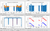 |
Fig. 1. Current look of our self-developed unique light- and ETV-curve analyzer GUI. In the top left corner, the raw light curve is plotted (blue) alongside the fitted trends (orange). In the top right corner, the detrended light curve is plotted after the normalization by the previously fitted trends. In the lower left corner, the previously detrended and normalized light curve binned and folded with the specified bin numbers and ephemeris is plotted alongside the polinomial templates fitted on the two types of eclipses. Finally, in the lower right corner, the ETVs calculated from the primary (red) and secondary (blue) mid-eclipse times using the indicated ephemeris from the top are plotted. Below each panel are several useful features (see the text for details) that enable a fast interactive analysis of any set of light curves. |
3. Analysis
3.1. Theoretical basics of the ETV analysis
The ETVs were modeled in a very similar manner to what was described in Borkovits et al. (2015, 2016). The full analytic model takes the form
![Mathematical equation: $$ \begin{aligned} \Delta =\sum _{i=0}^{3}c_{i}E^{i}+[\Delta _{\mathrm{LTTE} } +\Delta _{\mathrm{dyn} }+\Delta {\mathrm{apse} }]_{0}^{E}, \end{aligned} $$](/articles/aa/full_html/2024/05/aa48909-23/aa48909-23-eq2.gif) (2)
(2)
where the polynomial term contains corrections for the calculated eclipse times (in the case of i = 0, 1), constant rate, and linear period variations (in the case of i = 2, 3). The constant and linear (i = 0, 1) terms were used for all the sources in our analyses. In contrast to this, the i = 2, 3 polynomial terms were fit only in a few cases, where a quadratic or even more complicated additional variations in the ETV curves were evident.
Moreover, the (ΔLTTE, dyn, apse) terms represent the contributions of LTTE, P2 timescale dynamical perturbations, and apsidal motion, respectively, while the square bracket denotes the difference of each term measured in the Eth and zeroth (i.e., reference) cycle. For consistency, we provide only very brief descriptions and the formulae of these latter terms as they were used. A detailed explanation can be found in Borkovits et al. (2015, 2016).
3.1.1. Light travel-time effect
The classical LTTE (or Rømer delay) contribution comes from the periodically varying distance of the inner binary during its orbital revolution around the common center of mass of the triple system that causes a periodic variation in the light travel time toward the observer. This is detected as a periodic ETV. Based on Irwin (1952), this was taken into account in the form of
 (3)
(3)
where i2, e2, v2, and ω2 refer to the inclination, eccentricity, true anomaly, and the argument of periastron of the outer orbit1 (i.e., the relative orbit on which the tertiary star orbits the center of mass of the inner binary), respectively, while aAB stands for the semimajor axis of the (physical) orbit of the center of mass of the inner pair around the center of mass of the whole triple system. Finally, c denotes the speed of light.
It can easily be shown that when the orbital elements of the outer orbit remain constant, this effect can be described with a pure sine in the eccentric anomaly domain, whose amplitude is
 (4)
(4)
By analogy with the mass function used for single-lined spectroscopic binaries (SB1), the mass function is commonly introduced as
 (5)
(5)
where in the last form, the numerical constant is correct when time is expressed in days and masses are expressed in solar mass. (Here and hereafter, mA, B, C denote the individual masses of the three constituent stars, while mABC stands for the total mass of the triple system.)
In regard to the wide or outer orbit, an LTTE solution carries exactly the same information as can be extracted from the radial velocity measurements of a single-line spectroscopic binary (SB1). Therefore, in addition to the orbital period of the outer orbit (P2), we can determine three of the six orbital elements of the outer orbit (e2, ω2, and τ2), and moreover, the projected semimajor axis of the inner pair orbit around the common center of mass of the triple (aAB sin i2), from which in the absence of any external information, we can determine the mass of the third companion as a unique function of two additional parameters, namely, the total mass of the inner binary mAB, and the orbital inclination (i2). This external information might have come from the observations of radial velocities of the third star (producing a quasi-SB2-like system), and/or from detection of third-body eclipses (a good example for both situations is e.g., HD 181068, Borkovits et al. 2013) or from the detection of dynamically driven ETVs in tight triple systems. When no external information like this was available for the total mass of the inner pair, in the case of W UMa-type, that is, for overcontact binaries, we estimated the binary mass with the use of the empirical mass-period relations of Gazeas & Stȩpień (2008), while for other systems, we simply set mAB = 2 M⊙.
3.1.2. P2 timescale dynamical perturbations
The contribution of dynamical perturbations comes from the possible gravitational interaction between the outer component and the inner binary, which can result in the change of the orbital parameters of the inner binary and hence in a period variation. While LTTE terms were fit by default during our analysis, the P2 timescale dynamical contributions were taken into account only when the tightness of the system under investigation made it necessary. The most elaborate presentation of the theory of the P2− (medium-) timescale perturbations and their manifestations in the ETV of a tight EB was presented and discussed in Borkovits et al. (2015). For the sake of brevity, we repeat here only the lowest order (i.e., most significant) quadrupole terms (which slightly modifies Eqs. (5)–(11) of Borkovits et al. 2015), while higher-order (and more lengthy) formulae can be found in the appendices of Borkovits et al. (2015). According to this theory, the quadrupole-level dynamical contribution to an ETV curve in a CHT is
![Mathematical equation: $$ \begin{aligned} \Delta _{\rm dyn}=&\mathcal{A} _{\rm dyn}\left(1-e_1^2\right)^{1/2} \left\{ \left[f_1+\frac{3}{2}K_1\right]\mathcal{M} \right.\nonumber \\&+\left(1+I\right)\left[K_{11}\mathcal{S} (2u_2-2\alpha )-K_{12} \mathcal{C} (2u_2-2\alpha )]\right] \nonumber \\&+\left(1-I\right)\left[K_{11}\mathcal{S} (2u_2-2\beta )+K_{12} \mathcal{C} (2u_2-2\beta )]\right] \nonumber \\&+\sin ^2i_{\rm m}\left(K_{11}\cos 2n_1+K_{12}\sin 2n_1\right.\nonumber \\&\left.\left.-\frac{4}{3}f_1-2K_1\right) \left[2\mathcal{M} -\mathcal{S} (2u_2-2n_2)\right]\right\} \nonumber \\&+\Delta _1^*(\sin i_{\rm m}\cot i_1), \end{aligned} $$](/articles/aa/full_html/2024/05/aa48909-23/aa48909-23-eq6.gif) (6)
(6)
where
 (7)
(7)
stands for the characteristic amplitude of the dynamical effects on a timescale equal to the outer period (P2). Furthermore, I = cos im denotes the cosine of the mutual or relative inclination (im), that is, the angle between the inner and outer orbital planes, while u2 = v2 + ω2 stands for the true longitude of the third star measured from the ascending node of the wide orbit with respect to the tangential plane of the sky. Moreover, the node-like quantities n1, 2 represent the angular distances of the intersection of the two orbital planes (i.e., the dynamical node) from the intersections of the respective orbital planes with the tangential plane of the sky (i.e., the observable nodes), while α = n2 − n1 and β = n2 + n1 (see Fig. 1 of Borkovits et al. 2015, for an easy visualization). Furthermore, the trigonometric terms depending on the parameters of the outer orbit (and the current position of the third star) are
 (8)
(8)
![Mathematical equation: $$ \begin{aligned}&\mathcal{S} (2u_2)=\sin 2u_2+e_2 \left[\sin (u_2+\omega _2)+\frac{1}{3}\sin (3u_2-\omega _2)\right], \end{aligned} $$](/articles/aa/full_html/2024/05/aa48909-23/aa48909-23-eq9.gif) (9)
(9)
![Mathematical equation: $$ \begin{aligned}&\mathcal{C} (2u_2)=\cos 2u_2+e_2 \left[\cos (u_2+\omega _2)+\frac{1}{3}\cos (3u_2-\omega _2)\right], \end{aligned} $$](/articles/aa/full_html/2024/05/aa48909-23/aa48909-23-eq10.gif) (10)
(10)
where l2 is the mean anomaly of the outer orbit. Moreover, the quantities depending on the inner orbit are
 (11)
(11)
 (12)
(12)
 (13)
(13)
 (14)
(14)
and, finally,  stands for the usually negligibly small precession terms, which are not shown here. They were taken into account during the analytic fitting process, however. (The upper signs refer to the primary eclipses, and the lower signs stand for the secondary events.)
In the case of a circular inner orbit (which occurs frequently for close binary stars, and hence, for most of the EBs), all the K functions disappear, and moreover, f1 reduces to unity, resulting in a much simpler equation for Δdyn.
The Δdyn term was only included in the ETV analysis when the tightness (i.e., the ratio P2/P1) of the triple system made it necessary. In several cases, typically for the tightest, eccentric, and/or inclined triples, the shapes of the ETV curves showed even at the first inspection that the dynamical effects are strong or dominant. For some other cases, however, the need to include dynamical effects was far from evident. For all the LTTE-only fit ETVs, the software therefore automatically calculated the nominal amplitude ratio of 𝒜dyn/𝒜LTTE under the assumption that mAB = 2 (discussed above) and i2 = 90°, the latter of which yields the minimum value of the amplitude ratio. When this ratio was found to be higher than 0.25, we repeated the fitting process and switched the dynamical contribution on.
The dynamical ETV terms theoretically give much more orbital, geometric, and other dynamical parameters than a pure LTTE-dominated ETV solution because the dynamical terms simultaneously depend not only upon the orientations of both orbits relative to the observer, but also upon the orientations of the two orbits relative to each other (as the gravitational perturbations are driven by the relative positions of the three stars with respect to each other). The dynamical terms therefore give the full three-dimensional spatial configuration of the triple system, including a key parameter such as the mutual (or relative) inclination (im) of the inner and outer orbits. Moreover, in the amplitude of the dynamical ETV, the outer mass ratio (q2 = mC/mAB) also occurs, and moreover, the outer inclination i2 can be obtained as well. Thus, with the combination of the LTTE and dynamical terms, mC and mAB can also be determined directly. Unfortunately, however, the parameter space of a combined LTTE and dynamical ETV solution is so complex and multiply degenerate that in the absence of any other external information, we cannot expect an accurate mass determination from this combination of contributions to the ETV. A detailed discussion of the parameters that can be retrieved from a dynamical LTTE solution can be found in Borkovits et al. (2015), while the degeneracies of these combined ETV solutions are discussed by Rappaport et al. (2013) and Borkovits et al. (2015).
3.1.3. Apsidal motion
Apsidal motion (i.e., the rotation of the orbital ellipse within the orbital plane) may have several different origins. The most frequent and well-known variations are the relativistic, classical tidal (arising from the nonspherical mass distribution of the tidally deformed bodies), and the dynamical (third-body perturbed) apsidal motions (see, e.g., Borkovits et al. 2019a, for a short review). Regardless of the origin of this phenomena, its effect on the ETV curves can be described mathematically as follows:
![Mathematical equation: $$ \begin{aligned} \Delta _{\rm apse}=&\frac{P_1}{2\pi } \left[2\arctan \left(\frac{\pm e_1\cos \omega _1}{1+\sqrt{1-e_1^2}\mp e_1\sin \omega _1}\right)\right.\nonumber \\&\left.\pm \sqrt{1-e_1^2}\frac{e_1\cos \omega _1}{1\mp e_1\sin \omega _1}\right]. \end{aligned} $$](/articles/aa/full_html/2024/05/aa48909-23/aa48909-23-eq16.gif) (15)
(15)
(The form of this equation in widespread use is given as a trigonometric series in ω1. The slight dependence on inclination angle is also taken into account in Gimenez & Garcia-Pelayo 1983.)
For tight triples and especially for triples with less compact inner pairs, the dynamically forced apsidal motion generally dominates the other two contributions substantially. We show in Sect. 4 that for all of the currently investigated triples with eccentric inner binaries, this is the actual scenario. Instead of fitting a (linear) apsidal advance rate (Δω1), hidden in Eq. (15), as an additional free parameter, we therefore calculated the current values of ω1 (and also of e1) inherently for each time during the fitting process, with the use of the perturbation equations, and in the way described in Borkovits et al. (2015).
3.2. Methods of the ETV analysis
The software package that realizes the mathematical model discussed above is described in detail in Borkovits et al. (2015), and it was previously applied in several studies to analyze ETV curves of several Kepler (Borkovits et al. 2015, 2016), K2 (Borkovits et al. 2019b), CoRoT (Hajdu et al. 2017), OGLE (Hajdu et al. 2019), and TESS (Borkovits et al. 2021; Pribulla et al. 2023) EBs. When the medium-period dynamical ETV contribution did not need to be included in the systems (Sect. 3.1.2), we applied a simple Levenberg-Marquardt-type (LM) differential least-squares parameter optimization to find the most probable solution. (The advantages and disadvantages of the use of this method for the current problem and some further details are discussed by Borkovits et al. 2015.)
When the dynamical contribution needed to be included, we followed a different parameter optimization technique. Because of the large number of parameters to be fit and because they are highly nonlinearly correlated, this is not an ideal situation for the LM method. Therefore, we switched to a Markov chain Monte Carlo (MCMC) approach. This is a novelty of the software package relative to its formerly used versions. In this way, we were able to explore the whole (or at least the physically realistic) part of the parameters and obtain more realistic uncertainties.
4. Results and discussion
As was mentioned in Sect. 2, we identified 351 EBs in total whose ETVs exhibited promising nonlinear variations. In order to identify already known triple systems or candidates in our sample, we thoroughly searched the literature of these 351 EBs. We found five formerly known EBs for which previous ETV studies (based on former ground-based observed eclipse times) indicated an additional, more distant component. These are TIC 219109908 (EF Dra, Yang 2012), TIC 219738202 (BX Dra, Park et al. 2013), TIC 233532554 (RR Dra, Wang & Zhu 2021; Şenavcı et al. 2022), TIC 298734307 (HL Dra, Shi et al. 2021), and TIC 288734990 (NSVS 01286630, Wolf et al. 2016; Zhang et al. 2018). In the first four cases, however, the previously found third-body periods are in the range of decades, and the currently found short-term nonlinear ETV behaviors therefore cannot be accounted for by these putative companions, while although the outer orbital period is on the same order as in our solution for the last system, the TESS ETV data, and hence, our solution disagrees with the former results. For nine other objects in our candidate sample, we found some external archival eclipse times, but there were no actual earlier ETV studies of these objects.
In conclusion, out of the promising 351 EBs, we identified 135 hierarchical triple system candidates for which the CHT nature appears to be almost certain, and another 77 systems that are at least moderately likely CHT candidates. The remaining 58 EBs are less likely cases. In Fig. 2 we plot the locations of these 77 likely CHT candidates in the P1 vs. P2 plane, where for comparison, we also plot some previously known CHTs from some other surveys. Moreover, we plot the ETV curves together with the best analytic LTTE or combined LTTE+dynamical fits for all the 135 systems in Appendix A.
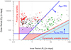 |
Fig. 2. Locations of the analyzed hierarchical triple star candidates together with other triples, detected with the space telescopes Kepler and TESS in the P1 − P2 plane. The black and red dots and green squares represent the current NCVZ candidates. For the black and red systems, simple LTTE solutions were satisfactory, while for the green systems, the dynamical effects were also taken into account. (The red symbols denote the most uncertain solutions, which were omitted from the statistical investigations.) The gray dots and squares denote the same classes of hierarchical triple star candidates as in the original Kepler-field, which were analyzed in Borkovits et al. (2016). The gray triangles represent recently discovered K2 and TESS systems with accurately known photodynamical solutions. (These are mostly triply eclipsing triple systems.) The vertical red line at the left side shows the lower limit of the period of overcontact binaries. The horizontal and sloped blue lines are boundaries that roughly separate detectable from undetectable ETVs. The detection limits were again set to 50 s. These amplitudes were calculated following the same assumptions as in Fig. 8 of Borkovits et al. (2016), that is, mA = mB = mC = 1 M⊙, e2 = 0.35, i2 = 60°, ω2 = 90°. The arrows indicate the direction of the increase in the respective amplitudes. The shaded regions from left to right represent (i) the W UMa desert, which is the (almost) empty domain in which a tight third companion of a short-period EB would certainly be detectable through its LTTE, even in the absence of a measurable dynamical delay, (ii) the purely dynamical region, in which the dynamical effect should be detectable while the LTTE would not, and (iii) the dynamically unstable region in the sense of the Mardling & Aarseth (2001) formula. While the border of this latter shaded area was also calculated with e2 = 0.35, we also give the limit for e2 = 0.1 as the thinner red line within this (light blue) region. |
We first present our findings for the purely LTTE and the combined LTTE+dynamical solution systems in general below. We then discuss some specific subgroups of the newly discovered CHT candidates.
4.1. Triple system candidates with purely LTTE solutions
From the ETVs of the narrowed sample of the 135 good CHT candidate systems, we identified 94 EBs for which we were able to find purely LTTE solutions. According to the reliability of the solutions, we divided these systems into three groups. Into the first group, we ranked the 19 EBs for which we judged our LTTE solutions to be certain or at least highly likely. These are typically close and likely triple systems in which the period of the third component (i.e., the outer period) does not exceed half of the nominal ∼1278-day length of the complete TESS NCVZ data set, the amplitude of the ETV curve(s) is substantially higher than the scatter of the individual ETV points, and finally, all the sensitive sections of the light-time orbits are well covered. While the first two criteria look trivial, we had to introduce the third criterion because of the large intermediate gaps in the observations between sectors 26 and 40 and between sectors 41 and 47. An example of the CHT candidates for which this last criterion was applied is TIC 159398028. Despite its outer period of P2 = 671 ± 3 d, this system was only ranked in the second (less certain) group because none of the lower ETV extrema and only one of the two upper extrema was covered by the observations. The outer P2 periods of the third companions are in the range of 109 and 628 days. All these compact triples have very close inner EBs (there are only three inner pairs with P1 > 1 days). This is expected because for longer inner periods, these compact systems would have dynamically dominated ETVs. We tabulate the main parameters of the LTTE solutions of this group in Table 1. The uncertainties of each parameters are given in parentheses and refer to the last digit(s). As the purely LTTE solutions were calculated with nonlinear LM optimization, these are formal uncertainties obtained via matrix-inversion and the resultant correlation matrices after reducing the χ2s to unity. In the last three columns, we list the minimum third-body mass (mC)min, the nominal dynamical to LTTE amplitude ratio,  , calculated with the use of this minimum mass, and finally, the assumed mass of the binary, mAB, which was used to calculate the minimum of the outer mass and the amplitude ratio. When the total mass of the inner binary is known from the literature, the value is given together with the current references, but in most cases, we only list some realistic estimate (which we denote with a colon after the numerical value).
Triple system candidates with certain or very likely LTTE solutions.
We classified 17 additional systems with less certain but likely LTTE solutions. These systems are CHTs with a high certainty, but do not fulfill all the criteria that were required for the first group. Their outer periods are between 507 and 1011 days, which means that more than one full orbit is covered at least partly in all cases. All but four systems have inner periods shorter than one day. They are listed in Table 2.
Triple system candidates with less certain but likely LTTE solutions.
Finally, in Table 3, we tabulate the parameters of the LTTE solutions of the remaining 58 systems. This is a very inhomogeneous group. In the case of some EBs, the LTTE solution looks quite reasonable, but when the period is certainly longer than the duration of the dataset, the parameters we obtained are likely not very robust. In other cases, however, even the interpretation of the nonlinear ETVs as LTTE signals seem suspect. Strictly speaking, because we were able to obtain any LTTE solutions, it does not follow that there is any third component in the given systems. Therefore, this third set should only be considered with great caution, and we do not recommend using the numerical results of this subgroup for any statistical studies. Instead, the group of these systems should only be considered as EBs that display clearly nonlinear ETVs and are therefore worthy of further attention.
Triple system candidates with very uncertain and questionable LTTE solutions.
4.2. Triple system candidates with combined LTTE and dynamical solutions
For 41 EBs we obtained combined LTTE and dynamical ETV solutions. The inferred outer periods in this group range from 68 days to ∼4000 days. Similar to the pure LTTE systems, we again considered the solutions of the 27 triples certain whose outer period did not exceed half the length of the given data set (see Table 4). (The same caution as was discussed in case of the LTTE systems must be taken into account here as well.) The nominally less certain solutions of the remaining 14 systems are tabulated in Table 5.
Orbital elements from combined dynamical and LTTE solutions with an outer period shorter than half of the length of the data sets.
Orbital elements from less certain combined dynamical and LTTE solutions.
The structure of these Tables 4 and 5 slightly departs from that of the three tables of LTTE triples (Tables 1–3). This agrees with the fact that from a combined solution, we can determine individual masses (at least mC and mAB), and the semimajor axis of the outer orbit (a2) can therefore also be readily calculated. Moreover, in these tables instead of a theoretically calculated, nominal dynamical to LTTE contribution amplitude ratio, we give the true measured ratio of 𝒜dyn/𝒜LTTE, which can directly be determined from the analytic ETV solution curves. Because of the large number of the parameters that can be obtained from such a dynamical solution, we also introduce Table 6, where we list additional parameters for the combined solution systems. These are mainly the apsidal motion and/or orientation and nodal precession parameters of these triples. In this regard, however, some caution should be taken as follows.
Apsidal motion and/or orientation parameters from AME and dynamical fits.
First, as was discussed by Borkovits et al. (2016) in the context of the mutual inclination (im) parameter, we can practically not distinguish between, for example, an im = 0° and im = 10° ETV solution, at least not on the timescale of TESS observations. From an observational point of view, however, there may be strong differences between the two solutions, as the second one may result in rapid inner inclination (i1) and hence eclipse depth variations, and therefore, they should be clearly distinguishable. Hence, in all cases, when our solution resulted in such a mutual inclination value that disagreed with the rate of the observed EDVs (including non-EDV cases), we did not accept the solution and forced a coplanar (im = 0°) solution.
Second, the tabulated inner inclinations (i1) should also be considered with great caution. The dynamical ETV solution, especially for coplanar cases, is almost insensitive to this parameter. Hence, it is better to fix its value a priori. Since for the vast majority of the combined LTTE+dyn systems no light curve solution is available, i1 generally is an unknown parameter. Fortunately, however, most of the dynamics-dominated systems have longer inner periods (see below), and hence, we do not expect to obtain large errors by assuming inclinations of i1 ∼ 87° −89°, as we have done.
The comparison of these triple systems with the purely LTTE triples shows that they contain fewer close inner binaries in general. (The mean and the median of the inner periods are  and
and  , respectively.) This property may arise for different reasons. For example, the amplitude of the dynamical ETV contribution is proportional to
  , that is, in addition to the tightness (P1/P2) of the system, it also scales with the inner period. Among two similarly tight triples, the longer-period triple therefore produces ETVs with a larger amplitude that can better be detected (assuming that the other orbital and dynamical parameters are similar). This fact may at least in part explain the lack of tight triple systems containing the closest binaries. Moreover, in the case of the closest binaries, tidal effects might be effective enough to circularize the inner orbits, and therefore, most of the observed closest binaries revolve on circular orbits or on orbits with a very low eccentricity. Again, this can effectively reduce the amplitudes of the dynamical terms (Borkovits et al. 2011), which again may explain the lack of the detection of triples (at least via ETV) in the light red region of Fig. 2. On the other hand, for somewhat wider inner EBs, the more distant third companions that would produce purely LTTE-generated ETVs must have orbital periods in the range of at least a few years. They can therefore not be detected with high confidence during the three-year-long and noncontinuous observations of the NCVZ by TESS. Consequently, the purely LTTE triple star candidates should be offset toward systems with a shorter inner period, that is, closest systems.
4.3. Systems of special interest
We discuss below some small subgroups of the identified triple star candidates that are of special interest for different reasons.
4.3.1. Tightest triples
We found five systems with P2/P1 ≲ 20. These are TICs 236774836 (with P2/P1 ∼ 9.35), 219885468(14.7), 389966039(16.3), 235934882(18.6), and 233684019(19.9). (In Fig. 2 these systems are represented with the five green rectangles that are closest to the border of the dynamically unstable domain in the lower right part of the plot). Despite the weakly hierarchical nature of these triples, our analytic hierarchical three-body models fit and describe these ETVs fairly well. However, according to our prior experiences with Kepler systems, our analytic hierarchical triple star model becomes less accurate for these tight triplets on a somewhat longer timescale of a decade (which in general is about the timescale of the apse-node type or long-period perturbations of these triples), suggesting that the analytic model of this latter class should be improved). In this regard, TIC 219885468 serves as a good case study of this effect because recently, Borkovits & Mitnyan (2023) carried out a more complex photodynamical analysis of this triple star system. During this analysis, the motion of the triple star system is integrated numerically, and we can therefore compare our analytical results with the output of the more exact numerical integration. Regarding the masses, Borkovits & Mitnyan (2023) obtained  and
and  (while the analytical model resulted in
  and
and  , respectively). The eccentricities2 also agree well (
 vs.
vs.  ) and (
 vs.
vs.  ). Similarly, the arguments of periastron of the inner orbit are quite close to each other in the two solutions (
 vs.
vs.  ). In contrast to this, at first sight, the discrepancy in the arguments of periastron of the outer orbit is remarkable (
 vs.
vs.  ). However, this difference is close to 180° and can be understood from the point of view that the analytic perturbation formulae only depend upon 2ωout and are therefore insensitive to a 180° difference in ω2. On the other hand, the LTTE term depends on ω2, which might have resolved this ambiguity in general, but in the current situation, the LTTE contribution is only about 2 − 3% of the dynamical contribution to the ETV. Our analytical solution therefore still suffers from this ambiguity. In conclusion, our approximate analytical ETV solutions appear to be quite acceptable even for these tight triples. On the other hand, however, for the some decade-long evolution (i.e., apsidal motion) of the current (and also other similarly tight) systems, we again refer to Borkovits & Mitnyan (2023), who pointed out that there are some discrepancies between the analytically predicted and numerical integrated apsidal motion periods (for the current system
  yr vs.
  yr). Hence, future follow-up observations and then numerical integration and modeling of the triple star motion of these tight systems would be especially important.
4.3.2. Triple star candidates with eclipse-depth variations
We identified eight triple star candidates where the inner EBs exhibit EDVs. These systems are TICs 233684019, 233729038, 236774836, 259004910, 288611133, 357686232, 417701432, and 441768471. The strongest variation is found in TIC 236774836, which is the tightest triple system candidate in our entire sample (with P2/P1 ∼ 9.35). While during the year 2 observations, the eclipse depths in this source remain constant, a dramatic decrease in the eclipse depths occurred in the year 4 data and the eclipses completely disappear near the beginning of year 5 (sector 56). The most likely explanation for this rapid EDV is a noncoplanar configuration of the given triple system that forces precession of the orbital planes and consequently, variation in the inclination of the EB. As the timescale of such an effect is proportional to  , one can expect the detection of such a rapid effect in the tightest and most compact triple systems. Finally, we note that TIC 230002837 also exhibits slight suspicious EDVs, but we were unable to find any reliable (or at least uncertain) third-body solution for its ETVs.
4.3.3. Eccentric eclipsing binaries with detectable apsidal motion
We found eccentric EB (eEB) orbits in 27 candidate systems (see Table 6). All of them belong to the systems with a combined LTTE+dynamical ETV solution. In an eEB, apsidal motion is expected. While the eccentricity of an EB orbit can generally be discerned simply by visual inspection of a possibly unequal time interval between the odd-even and even-odd eclipse events and/or the different durations of the even and odd eclipses, the apsidal motion most readily reveals itself via the divergence or convergence of the primary and secondary ETV curves (which is the manifestation of the anticorrelated behavior of the primary and secondary ETV curves in a time interval that is substantially shorter than the period of the apsidal precession). Because the duration of the nominally ∼1300 d TESS observations is very short relative to the decades to millennia long tidal and relativistic apsidal motion periods, no detection of apsidal motion caused primarily by these effects in our ETV curves is expected. Thus, where we clearly detect apsidal motion in our short-term ETVs, we can be certain that this effect is due to rapid dynamically forced apsidal motion.
We identified clear apsidal motion in ten systems. These are TICs 199616648, 219771659, 219885468, 233684019, 233729038, 233738966, 236774836, 256514937, 357686232, and 417701432. In some other systems, the ETVs suggest apsidal motion as well, but the detection is less certain since the P2 period dynamically forced ETVs may hide the convergence or divergence of the two ETVs. These seven systems are TICs 236769201, 243337122, 259271740, 272705788, 288611133, 376976908, and 441768471.
In Table 6 we list the theoretical dynamical apsidal motion periods (Papse) that were calculated by our software using the quadrupole-order perturbation theory of the hierarchical three-body problem (see Borkovits et al. 2015, Appendix C, for a detailed description). The shortest theoretical apsidal motion period is Papse = 9.6 yr. It was detected in TIC 236774836, that is, in the system in which the eclipses completely disappeared for 2022 (see in Sect. 4.3.2 above).
Moreover, our software package calculated the theoretical dynamical apsidal motion for all noncircular dynamically dominated ETVs, and Papse is therefore tabulated in Table 6 for all eEBs, regardless of whether the apsidal motion manifests itself during the short interval of TESS observations. This shows four systems for which the given Papse value is negative. Here, the negative sign denotes retrograde apsidal motion. While the tidal and relativistic apsidal motions are always prograde (i.e., the orbital ellipse revolves in the same direction as the orbiting bodies), dynamically forced apsidal motion can be retrograde for either dynamical or geometric reasons (see, e.g. Borkovits et al. 2022).
4.3.4. Triply eclipsing triples
We found third-body eclipses in four systems. These are TICs 229785001, 233684019, 288430645, and 441738417. Their third-body periods range from 145 to 472 days. The periods deduced from the ETV curves agree with the locations of the additional eclipses in all the four systems, confirming that the same objects are the origin of the additional eclipses and the timing variations. A detailed photodynamical analysis of TIC 229785001 was published earlier by Rappaport et al. (2023). The results of our analytic ETV solution agree well with their results. We plan complex photodynamical investigations of the remaining three systems in the near future.
4.3.5. Interpretation of the peculiar eclipse-timing variation curve of GZ Draconis
While GZ Draconis does not appear to be an extremely interesting peculiar triple system, we nonetheless feel it worthwhile to discuss the cautionary tale of this quite average EB. This relatively bright (V = 9.4) object was first known as a visual double star in the 1980s (see, e.g. Muller 1984; Heintz 1987), and the EB nature of the brighter component was then discovered by the HIPPARCOS satellite (Kazarovets et al. 1999; Fabricius & Makarov 2000). The system was observed continuously in two-minute cadence mode during years 2, 4, and 5 of TESS observations. From our point of view, only the ETV curves calculated from the TESS-observed primary and secondary eclipses are important. The year 2 observations already showed clear third-body-induced ETVs in the timing diagrams. By the end of the year 2 observations, and using some previous less accurate times of primary eclipses, calculated from the publicly available SuperWASP (Wide Angle Search for Planets) observations, we were able to find a reasonably good LTTE solution with a period of P2 = 476 ± 1 d. We found an unexpected dip in the primary ETV curve around BJD ∼2 458 800, however, with an amplitude of  and duration of ∼40 days, but we did not think this feature important, assuming that it was caused by some light-curve distortions (e.g., spottedness). This dip cannot be seen in the much less accurate secondary ETV curve. Then, the new NCVZ monitoring of TESS began during the second year of the first extended mission, and the new eclipse times confirmed the former ETV solution sector by sector. The uninteresting characteristics of this straightforward ETV curve changed immediately when the sector 53 observations became available, and we calculated the new set of eclipse times. The same dip in the ETV curve as in the year 2 data occurred again and in the very same phase of the third-body orbit as two outer orbital cycles earlier (Fig. 3). By this time, we realized that even though the P2/P1 ratio of ∼211 is high (i.e., not a very tight triple), the dynamical effect might still produce a non-negligible contribution to the ETV curve and explain the unexpected additional dips3. A further, more in-depth consideration of the shape of the ETV curve makes this possibility even more exciting. The other (bottom) extrema of the ETV curves show that during these phases in year 2 (between about JDs 2 458 930 and 2 459 000) and year 5 (JDs 2 459 880 – 2 459 950), the curvatures of the ETVs practically disappear, which suggests the presence of a second bump that counteracts the LTTE. Therefore, we may assume two bumps within one outer period (for the dynamical curve), which, in the case of a circular inner orbit (as is the case in GZ Dra), may only occur when the two orbital planes are substantially inclined to each other (see Eq. (46) of Borkovits et al. 2003). Thus, the shape of the ETV suggests that there is an exceptional opportunity in the case of GZ Draconis for determining the mutual inclination purely from the ETV for this non-tight triple star system. Then, our search for an inclined combined LTTE and dynamical ETV solution became quite fruitful, and we realized that this triple star must be one of the currently most strongly inclined triple star systems known with im = 58° ±7°.
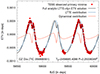 |
Fig. 3. Primary ETV curve of GZ Draconis, formed from the two-minute TESS measurements (red dots), together with the combined LTTE+dyn solution (black curve). We separately plot the LTTE (light blue) and quadrupole-order dynamical (light red) contributions. The unusual bumps near the upper extrema of the observed curves are clearly visible and indicate a significant noncoplanar dynamical contribution. See text for further details. |
Finally, in this regard, we make two additional notes. First, we refer to the fact that that this mutual inclination is well within the high mutual inclination domain of the original von Zeipel-Lidov-Kozai phenomena (see, e.g., Naoz 2016, and further references therein), where large-amplitude eccentricity cycles may occur. However, we cannot expect large-amplitude eccentricity variations like this in the currently circular inner pair because of the tidal interactions between the two components, which cancel the ZLK cycles.
Second, this high mutual inclination implies very large-amplitude orbital plane precession cycles, which would lead to substantial EDVs and also the disappearance (and later, reappearance) of the eclipses. While this may be true, Table 6 shows that the theoretical period of these variations in GZ Draconis (with the measured parameters) is about Pnode ∼ 3800 yr, which explains the absence of EDV during the few-year-long TESS observations.
4.4. Statistics
Borkovits et al. (2016) published the largest collection of CHTs with known orbital periods using a sample of 222 objects found in the Kepler field. We have about one-third of that sample size with 77 objects that are likely or very likely to be triples, but because we applied similar detection and analysis techniques, it may be worthwhile to perform a similar statistical analysis on our newly found systems in the TESS NCVZ and make a comparison.
In Fig. 4 we show the distribution of the outer orbital periods in our sample. Most systems have outer orbital periods of 100−800 days. Our photometric data sets contain smaller and larger gaps due to the observing strategy of TESS: the former are caused by the fact that the telescope changes its observational field of view every ∼27 days and it is not guaranteed that the object will continue to be observed in all sectors; while the latter are simply caused by the fact that TESS observes different hemispheres during alternating years. This observational strategy might cause the slightly higher number of systems with 100- to 800-day outer orbital periods as they are easier to detect with these data sets. The total temporal coverage of our data sets is about 1300 days, and the number of systems with longer orbital periods decreases more or less with  , as suggested by Borkovits et al. (2016).
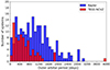 |
Fig. 4. Distribution of outer orbital periods for the Kepler (blue) and TESS NCVZ (red) samples. |
In Fig. 5 we plot the distribution of the outer eccentricities of systems in our sample. Except for six objects, all of them have an eccentricity value lower than 0.55, and the distribution looks more or less flat with some small fluctuations. It does not have similar characteristics to those of the distribution from the Kepler sample. Nevertheless, when we compare the cumulative eccentricity distribution (Fig. 6) with those from earlier studies, they are very similar to each other4 and completely different from simple linear or thermal distributions from theory. It resembles the distribution found by Duchêne & Kraus (2013) for populations of field EBs more closely.
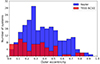 |
Fig. 5. Distribution of outer orbital eccentricities for the Kepler (blue) and TESS NCVZ (red) samples. |
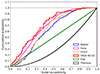 |
Fig. 6. Cumulative distribution of outer orbital eccentricities for our TESS NCVZ (red) systems along with samples from earlier studies, Kepler (blue), Gaia (magenta), and OGLE (orange), and theories, flat (green) or thermal (black) distributions. |
Figure 7 shows the relation between the outer orbital period and the outer eccentricity for both studies. The black line denotes a fit for a linear relation to the TESS NCVZ sample with a correlation of 0.05 (i.e., not very correlated), which is significantly lower than the value of 0.34 found by Borkovits et al. (2016) for the Kepler sample. We emphasize again, however, that our TESS sample is much smaller than the Kepler sample of Borkovits et al. (2016), and this is more expressively true for the longer outer period systems, where higher outer eccentricities are expected because they certainly cannot be detected at the current stage of the TESS sample.
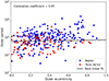 |
Fig. 7. Correlation of outer orbital periods and eccentricities for the Kepler (blue) and TESS NCVZ (red) samples. The correlation value only applies to the NCVZ set. |
In Fig. 8 we plot the distribution of the tertiary component masses (MC) for both our and the Kepler sample. For systems with measurable dynamical perturbations, exact masses can be determined, but for systems with LTTE, only minimum masses can be estimated from the mass function using the constraints on the inner binary mass explained in Sect. 3.1.1. Similarly to the Kepler sample, the majority of the systems with measured masses have tertiaries with a mass lower than 1.8 M⊙.
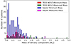 |
Fig. 8. Distribution of tertiary masses for the Kepler and TESS NCVZ samples directly measured from combined dynamical+LTTE ETV solutions (magenta and green, respectively) and lower limits estimated from pure LTTE solutions (blue and red, respectively). |
Figure 9 shows the correlation between the exact masses of the binary and the tertiary components for systems in which measurable dynamical perturbations occur for both our TESS NCVZ and the Kepler sample. The orange and blue lines represent the cases where all three components have the same mass, and where the mass of the tertiary equals the mass of the inner binary, respectively. The majority of the systems are located below or close to the orange line, while only four systems lie above the blue line, indicating that the tertiary has a higher mass than the inner binary components. In the Kepler sample, most the systems have an inner binary mass lower than 2 M⊙, while our TESS NCVZ sample contains only a handful of systems with inner binary masses like this, and most of the systems are above this value. Hence, these systems may serve as an extension to the regime of higher binary masses.
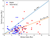 |
Fig. 9. Correlation of tertiary and inner binary masses for the Kepler (blue) and TESS NCVZ (red) samples with combined dynamical + LTTE ETV solutions. |
Figure 10 shows the distribution of the mutual inclination for systems in which the measurable dynamical perturbations allowed us to determine this quantity for both samples. The vast majority of the systems in our TESS NCVZ sample have a (nearly) coplanar configuration, and only a few systems can be found with higher mutual inclination values. This is different from the Kepler results, which showed a small peak centered at imut = 40°. However, in both cases, the results are somewhat hampered by small number statistics.
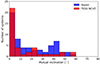 |
Fig. 10. Distribution of mutual orbital inclinations for the Kepler (blue) and TESS NCVZ (red) samples with combined dynamical + LTTE ETV solutions. |
Finally, in Fig. 11, we show the distribution of apsidal motion timescales for both samples.
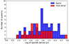 |
Fig. 11. Distribution of apsidal motion periods for the Kepler (blue) and TESS NCVZ (red) samples with combined dynamical + LTTE ETV solutions. |
4.5. Comparison with Gaia non-single star candidates
As recently demonstrated in Czavalinga et al. (2023), it is also possible to identify new hierarchical triple candidates using Gaia data comparing the orbital periods from the astrometric or spectroscopic Gaia NSS orbital solutions with the eclipsing periods from light curves and finding a difference of at least five times. For this purpose, we also cross-matched our full sample of 5139 objects with the Gaia DR3 non-single star catalog (Gaia Collaboration 2022). This yielded 32 and 116 matches with Gaia astrometric and spectroscopic orbital solutions, respectively. After the comparison of the orbital periods of the Gaia orbital solutions with the binary periods from the TESS light curves, we excluded 8 and 115 objects as the two types of periods were identical or exactly integer or half integer multiples of each other (i.e., Gaia picked up the EB period or its possible aliases because of limited Gaia data). This left a total of 25 triple candidates in our sample with an available Gaia orbital solution for the outer orbit of a possible tertiary component. As a final step, we analyzed the TESS light and ETV curves of these systems separately and excluded 10 further systems for various other reasons (e.g., the source was not an EB, or the light curve and the Gaia NSS solution belonged to another close star without a Gaia NSS solution). After all this, we found 15 systems with a Gaia NSS orbital solution, and moreover, the ETVs also confirm the validity of these solutions for all of them. For these objects, we list the orbital parameters from the two types of orbital solutions in Table 7. Five of these objects (TICs 229762991, 232606864, 237234024, 320324245, and 377105433) were found and recently published by Czavalinga et al. (2023), and our ETV solutions for these triples agree well with theirs, while the other 10 systems are new discoveries that also demonstrate the potential of the Gaia NSS catalog in the field of discovering new hierarchical triples. In Fig. 12 we plot the correlations of different orbital parameters determined from the two types of orbital solutions (Gaia NSS vs. ETVs) for the 22 systems found by Czavalinga et al. (2023) and the 10 systems newly found in our NCVZ analysis in a similar way as Czavalinga et al. (2023). These figures show that the 10 new systems found by us can further confirm the conclusions by Czavalinga et al. (2023), which is that Gaia reliably detects the correct outer orbital period, but the ETV results are often more accurate, especially in case of the outer eccentricity, projected semi-major axis and argument of periastron.
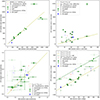 |
Fig. 12. Correlations between the orbital periods (upper left panel), projected semimajor axes (upper right panel), eccentricities (lower left panel), and arguments of periastron (lower right panel) from the Gaia NSS solutions and fitting LTTE models to the TESS ETVs of the NCVZ sample. Different colors show different types of Gaia NSS orbital solutions. The dashed yellow lines represent a ratio of unity, and in the bottom right panel, the dashed green line shows the ±180° difference between the arguments of periastron from the two types of solutions. In order to avoid breaking the dashed lines in the bottom right panel, we employed a ±360° shift for some of the ωout, NSS values, which is equivalent because of the periodicity of the argument of periastron. The faded dots are additional previously known systems from Czavalinga et al. (2023). |
Outer orbital parameters from the Gaia NSS and our TESS ETV solutions for the 15 triple candidates that have both solutions.
5. Summary
To discover new compact hierarchical triples, we have conducted a survey of EBs based on TESS data. We selected 3553 objects from a list of EBs found in the TESS data using a machine-learning approach. The objects are in or near the NCVZ of TESS and had sufficient photometric data. We obtained the light curves of every source from all available TESS sectors up to sector 60 in an automated way. After this, we used our newly developed Python GUI to visually confirm all of the light curves of our targets, determined their eclipsing periods, and calculated their ETV curves. We finally selected 351 objects for a further detailed analysis that seemed to have nonlinear ETVs that might be caused by previously unknown third bodies in these systems. Finally, we fit these ETVs with analytical formulae of LTTE or LTTE + dynamical perturbations.
We were able to derive models for 94 objects with purely LTTE and 41 objects with LTTE + dynamical solutions in total, which we divided into three and two subgroups based on the quality of the models. The first subgroup contained the most reliable, highly certain solutions for 19 and 27 objects with the two types of ETV solutions. The second subgroup had 17 and 14 objects with likely valid solutions, but with probably higher uncertainties in their orbital parameters. For the purely LTTE systems alone, the third subgroup consisted of 58 objects with very uncertain solutions that are still likely triple systems, but their parameters should be used with considerable caution. This is a total of 135 hierarchical triple candidates in our NCVZ sample, 10 of which were already known from previous studies, while the remaining 125 systems are new discoveries. A number of these systems are individually interesting. First, there are five very tight systems with a period ratio lower than 20, which are closest to the dynamical stability limit. It is worth noting that although our analytic models describe these systems well on the shorter timescale of the available TESS data set, they are inaccurate on decade-long timescales, and numerical integration of the orbits should be applied to model these systems correctly. There are also four triply eclipsing triples in our sample, one of which (TIC 29785001) was previously known. For this one system, our ETV solution is consistent with the previous solution of Rappaport et al. (2023). The other three systems are new discoveries. We plan a separate more detailed comprehensive analysis in the near future for them.
We outlined the case of GZ Dra, in which we have recognized and successfully modeled the previously unknown effect of dynamical perturbations. This analysis showed that GZ Dra is one of the most strongly inclined triple systems known, with im = 58° ±7°. Although this inclination is well within the range of the original von Zeipel-Lidov-Kozai effect, we cannot expect large-amplitude eccentricity cycles because of the strong tidal interactions between the components of the highly circularized inner pair. Nevertheless, we would expect large-amplitude orbital plane precession in the system, which would cause EDVs in its light curve, but the timescale of this variation is about one thousand years. We therefore cannot see its effect in the few-year-long TESS data set.
Because we also determined all the same parameters for every triple candidate in our sample, we were able to compare them with the distributions of Borkovits et al. (2016) for the full Kepler sample. For this purpose, we used only the 77 systems with a certain or likely valid ETV solutions (i.e., the first two subgroups). Our sample includes slightly more systems with an outer orbital period of 100−800 days, which is most likely caused by the observing strategy of TESS. For the outer eccentricities, we found that their cumulative distribution is similar to those found by earlier surveys (Kepler, OGLE, and Gaia), but very different from theoretical (flat and thermal) distributions. We did not find any correlation between the outer periods and eccentricities for the systems in our sample. We found that most of the masses of the outer components in our systems are below 1.8 M⊙ which is similar to the Kepler sample. Of the 41 systems with dynamical perturbations and for which exact masses can be derived for the components, we found that only 4 have a more massive tertiary component than their inner binaries. In the Kepler sample, the inner binary mass of most of the systems is lower than 2 M⊙, while in our sample, it is the opposite, complementing the regime of triples with higher inner binary masses. Similarly to what our other studies of TESS binaries have shown (Rappaport et al. 2023), the vast majority of these systems also have a negligible mutual inclination (i.e., coplanar configuration), and only a few systems have a distinctly nonzero mutual inclination. The latter also implies that we cannot see any peak at around 40°, as found by Borkovits et al. (2016) for the Kepler sample.
Finally, we crossmatched our list of targets with the Gaia NSS catalog and found 15 systems with either astrometric or spectroscopic orbital solutions with a substantially different orbital period than their eclipsing period. For all of these objects, our ETV solutions can confirm that they are triple systems, but 5 of them were already found and published by Czavalinga et al. (2023). We also confirmed the same correlations as Czavalinga et al. (2023) for the orbital parameters of these systems derived from the two different methods, and we can draw the same conclusions. The Gaia NSS catalog has great potential for discovering new hierarchical triples. The most reliable parameter in these solutions is the outer orbital period, while the other parameters can have larger uncertainties than was found via the ETV fits.
We demonstrated that TESS data in addition to many other applications are an excellent tool for finding and analyzing new hierarchical triple stars. Since many systems in our sample have uncertain solutions and more observations are required in order to improve their quality, we hope that TESS will continue monitoring these objects and that their reanalysis will become possible in the near future.
From now on, the orbital parameters with subscript 1 and 2 refer to the inner and the outer orbit, respectively.
Comparing the orbital elements, however, we recall that the definition and therefore the meaning of the orbital elements in a photodynamical and an analytical model are different. In the first, these are instantaneous osculating orbital elements at a given epoch, while in the analytic model, these are some type of averaged orbital elements for not necessarily the same epoch.
Similar dips can be seen in the dynamically contributed ETV curves of several other mostly Kepler-discovered triple systems (see, e.g., Borkovits et al. 2015, 2016; Gaulme et al. 2022).
The reason may be that cumulative distributions better hide statistical fluctuations that can dominate the appearance of a regular distribution.
Acknowledgments
This project has received funding from the HUN-REN Hungarian Research Network. T.M., T.B., T.H., and A.P. acknowledge the financial support of the Hungarian National Research, Development and Innovation Office – NKFIH Grants K-147131 and K-138962. This paper includes data collected by the TESS mission. Funding for the TESS mission is provided by the NASA Science Mission directorate. Some of the data presented in this paper were obtained from the Mikulski Archive for Space Telescopes (MAST). STScI is operated by the Association of Universities for Research in Astronomy, Inc., under NASA contract NAS5-26555. Support for MAST for non-HST data is provided by the NASA Office of Space Science via grant NNX09AF08G and by other grants and contracts. This work has made use of data from the European Space Agency (ESA) mission Gaia (https://www.cosmos.esa.int/gaia), processed by the Gaia Data Processing and Analysis Consortium (DPAC https://www.cosmos.esa.int/web/gaia/dpac/consortium). Funding for the DPAC has been provided by national institutions, in particular the institutions participating in the Gaia Multilateral Agreement. This publication makes use of data products from the Wide-field Infrared Survey Explorer, which is a joint project of the University of California, Los Angeles, and the Jet Propulsion Laboratory/California Institute of Technology, funded by the National Aeronautics and Space Administration. This publication makes use of data products from the Two Micron All Sky Survey, which is a joint project of the University of Massachusetts and the Infrared Processing and Analysis Center/California Institute of Technology, funded by the National Aeronautics and Space Administration and the National Science Foundation. We used the Simbad service operated by the Centre des Données Stellaires (Strasbourg, France) and the ESO Science Archive Facility services (data obtained under request number 396301).
References
- Babusiaux, C., Fabricius, C., Khanna, S., et al. 2023, A&A, 674, A32 [NASA ADS] [CrossRef] [EDP Sciences] [Google Scholar]
- Borkovits, T. 2022, Galaxies, 10, 9 [NASA ADS] [CrossRef] [Google Scholar]
- Borkovits, T., & Mitnyan, T. 2023, Universe, 9, 485 [NASA ADS] [CrossRef] [Google Scholar]
- Borkovits, T., Érdi, B., Forgács-Dajka, E., & Kovács, T. 2003, A&A, 398, 1091 [NASA ADS] [CrossRef] [EDP Sciences] [Google Scholar]
- Borkovits, T., Csizmadia, S., Forgács-Dajka, E., & Hegedüs, T. 2011, A&A, 528, A53 [NASA ADS] [CrossRef] [EDP Sciences] [Google Scholar]
- Borkovits, T., Derekas, A., Kiss, L. L., et al. 2013, MNRAS, 428, 1656 [NASA ADS] [CrossRef] [Google Scholar]
- Borkovits, T., Rappaport, S., Hajdu, T., & Sztakovics, J. 2015, MNRAS, 448, 946 [NASA ADS] [CrossRef] [Google Scholar]
- Borkovits, T., Hajdu, T., Sztakovics, J., et al. 2016, MNRAS, 455, 4136 [Google Scholar]
- Borkovits, T., Forgács-Dajka, E., & Rappaport, S. A. 2019a, EAS Publ. Ser., 82, 99 [CrossRef] [EDP Sciences] [Google Scholar]
- Borkovits, T., Rappaport, S., Kaye, T., et al. 2019b, MNRAS, 483, 1934 [NASA ADS] [CrossRef] [Google Scholar]
- Borkovits, T., Rappaport, S. A., Maxted, P. F. L., et al. 2021, MNRAS, 503, 3759 [NASA ADS] [CrossRef] [Google Scholar]
- Borkovits, T., Rappaport, S. A., Toonen, S., et al. 2022, MNRAS, 515, 3773 [CrossRef] [Google Scholar]
- Borucki, W. J., Koch, D., Basri, G., et al. 2010, Science, 327, 977 [Google Scholar]
- Carter, J. A., Fabrycky, D. C., Ragozzine, D., et al. 2011, Science, 331, 562 [NASA ADS] [CrossRef] [Google Scholar]
- Conroy, K. E., Prša, A., Stassun, K. G., et al. 2014, AJ, 147, 45 [NASA ADS] [CrossRef] [Google Scholar]
- Czavalinga, D. R., Mitnyan, T., Rappaport, S. A., et al. 2023, A&A, 670, A75 [NASA ADS] [CrossRef] [EDP Sciences] [Google Scholar]
- Derekas, A., Kiss, L. L., Borkovits, T., et al. 2011, Science, 332, 216 [NASA ADS] [CrossRef] [Google Scholar]
- Duchêne, G., & Kraus, A. 2013, ARA&A, 51, 269 [Google Scholar]
- Fabricius, C., & Makarov, V. V. 2000, A&A, 356, 141 [NASA ADS] [Google Scholar]
- Gaia Collaboration 2022, VizieR Online Data Catalog: I/357 [Google Scholar]
- Gaia Collaboration (Vallenari, A., et al.) 2023, A&A, 674, A1 [NASA ADS] [CrossRef] [EDP Sciences] [Google Scholar]
- Gaulme, P., Borkovits, T., Appourchaux, T., et al. 2022, A&A, 668, A173 [NASA ADS] [CrossRef] [EDP Sciences] [Google Scholar]
- Gazeas, K., & Stȩpień, K. 2008, MNRAS, 390, 1577 [NASA ADS] [Google Scholar]
- Gimenez, A., & Garcia-Pelayo, J. M. 1983, Ap&SS, 92, 203 [NASA ADS] [CrossRef] [Google Scholar]
- Hajdu, T., Borkovits, T., Forgács-Dajka, E., et al. 2017, MNRAS, 471, 1230 [NASA ADS] [CrossRef] [Google Scholar]
- Hajdu, T., Borkovits, T., Forgács-Dajka, E., et al. 2019, MNRAS, 485, 2562 [NASA ADS] [CrossRef] [Google Scholar]
- Hajdu, T., Matécsa, B., Sallai, J. M., & Bódi, A. 2022a, MNRAS, 516, 5165 [NASA ADS] [CrossRef] [Google Scholar]
- Hajdu, T., Borkovits, T., Forgács-Dajka, E., Sztakovics, J., & Bódi, A. 2022b, MNRAS, 509, 246 [Google Scholar]
- Heintz, W. D. 1987, ApJS, 65, 161 [NASA ADS] [CrossRef] [Google Scholar]
- Hippke, M., David, T. J., Mulders, G. D., & Heller, R. 2019, AJ, 158, 143 [Google Scholar]
- Irwin, J. B. 1952, ApJ, 116, 211 [Google Scholar]
- Kazarovets, E. V., Samus, N. N., Durlevich, O. V., et al. 1999, Inf. Bull. Var. Stars, 4659, 1 [Google Scholar]
- Kovács, G., Zucker, S., & Mazeh, T. 2002, A&A, 391, 369 [Google Scholar]
- Liakos, A., & Niarchos, P. 2017, MNRAS, 465, 1181 [NASA ADS] [CrossRef] [Google Scholar]
- Lightkurve Collaboration (Cardoso, J. V. D. M., et al.) 2018, Astrophysics Source Code Library [record ascl:1812.013] [Google Scholar]
- Mardling, R. A., & Aarseth, S. J. 2001, MNRAS, 321, 398 [NASA ADS] [CrossRef] [Google Scholar]
- Muller, P. 1984, A&AS, 57, 467 [NASA ADS] [Google Scholar]
- Naoz, S. 2016, ARA&A, 54, 441 [Google Scholar]
- Nelson, R. H. 2016, Inf. Bull. Var. Stars, 6164, 1 [NASA ADS] [Google Scholar]
- Pál, A. 2012, MNRAS, 421, 1825 [Google Scholar]
- Park, J.-H., Lee, J. W., Kim, S.-L., Lee, C.-U., & Jeon, Y.-B. 2013, PASJ, 65, 1 [NASA ADS] [CrossRef] [Google Scholar]
- Powell, B. P., Kostov, V. B., & Tokovinin, A. 2023, MNRAS, 524, 4296 [NASA ADS] [CrossRef] [Google Scholar]
- Pribulla, T., Borkovits, T., Jayaraman, R., et al. 2023, MNRAS, 524, 4220 [NASA ADS] [CrossRef] [Google Scholar]
- Rappaport, S., Deck, K., Levine, A., et al. 2013, ApJ, 768, 33 [NASA ADS] [CrossRef] [Google Scholar]
- Rappaport, S. A., Borkovits, T., Gagliano, R., et al. 2023, MNRAS, 521, 558 [NASA ADS] [CrossRef] [Google Scholar]
- Ricker, G. R., Winn, J. N., Vanderspek, R., et al. 2015, J. Astron. Telesc. Instrum. Syst., 1, 014003 [Google Scholar]
- Şenavcı, H. V., Čeki, A., Esmer, E. M., et al. 2022, Acta Astron., 72, 31 [Google Scholar]
- Shi, X.-D., Qian, S.-B., Li, L.-J., & Liao, W.-P. 2021, MNRAS, 505, 6166 [NASA ADS] [CrossRef] [Google Scholar]
- Stellingwerf, R. F. 1978, ApJ, 224, 953 [Google Scholar]
- Sun, W., Chen, X., Deng, L., & de Grijs, R. 2020, ApJS, 247, 50 [NASA ADS] [CrossRef] [Google Scholar]
- Tokovinin, A. 2021, Universe, 7, 352 [NASA ADS] [CrossRef] [Google Scholar]
- Toonen, S., Portegies Zwart, S., Hamers, A. S., & Bandopadhyay, D. 2020, A&A, 640, A16 [NASA ADS] [CrossRef] [EDP Sciences] [Google Scholar]
- Toonen, S., Boekholt, T. C. N., & Portegies Zwart, S. 2022, A&A, 661, A61 [NASA ADS] [CrossRef] [EDP Sciences] [Google Scholar]
- Wang, Z.-H., & Zhu, L.-Y. 2021, MNRAS, 507, 2804 [NASA ADS] [CrossRef] [Google Scholar]
- Wolf, M., Zasche, P., Kučáková, H., et al. 2016, A&A, 587, A82 [NASA ADS] [CrossRef] [EDP Sciences] [Google Scholar]
- Yang, Y.-G. 2012, Res. Astron. Astrophys., 12, 419 [CrossRef] [Google Scholar]
- Zhang, B., Qian, S.-B., Liao, W.-P., et al. 2018, Res. Astron. Astrophys., 18, 116 [CrossRef] [Google Scholar]
Appendix A: Plots of ETVs
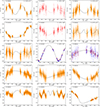 |
Fig. A.1. ETVs with third-body solutions. The ETV curves calculated from TESS observations of primary and secondary minima, and the average of the two, are denoted by red circles, blue boxes, and orange diamonds, respectively. We display and fit the ETV curves for both the primary and secondary eclipses only when the data quality warranted a joint analysis and the binary was eccentric. When the primary and secondary ETV curves are of comparable quality and the binary eccentricity is nearly zero, we display and fit only the average of the two ETV curves. When the quality of the primary ETV curve was significantly better than that of the secondary curve or when only primary eclipses are present, we present only the plot and the fit for the primary eclipses. Ground-based minima (taken from the literature, and available only for a few systems) are denoted by upward red triangles (primary) and downward blue triangles (secondary); their estimated uncertainties are also indicated. Purely LTTE solutions are plotted with black lines, and combined dynamical and LTTE solutions are drawn with gray lines. The use of quadratic or cubic terms is not indicated; for these and other details, see Table 1–5. |
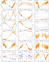 |
Fig. A.1. (continued) |
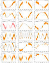 |
Fig. A.1. (continued) |
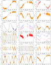 |
Fig. A.1. (continued) |
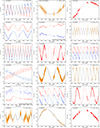 |
Fig. A.1. (continued) |
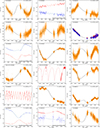 |
Fig. A.1. (continued) |
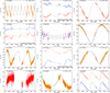 |
Fig. A.1. (continued) |
All Tables
Orbital elements from combined dynamical and LTTE solutions with an outer period shorter than half of the length of the data sets.
Outer orbital parameters from the Gaia NSS and our TESS ETV solutions for the 15 triple candidates that have both solutions.
All Figures
|
Fig. 1. Current look of our self-developed unique light- and ETV-curve analyzer GUI. In the top left corner, the raw light curve is plotted (blue) alongside the fitted trends (orange). In the top right corner, the detrended light curve is plotted after the normalization by the previously fitted trends. In the lower left corner, the previously detrended and normalized light curve binned and folded with the specified bin numbers and ephemeris is plotted alongside the polinomial templates fitted on the two types of eclipses. Finally, in the lower right corner, the ETVs calculated from the primary (red) and secondary (blue) mid-eclipse times using the indicated ephemeris from the top are plotted. Below each panel are several useful features (see the text for details) that enable a fast interactive analysis of any set of light curves. |
| In the text | |
|
Fig. 2. Locations of the analyzed hierarchical triple star candidates together with other triples, detected with the space telescopes Kepler and TESS in the P1 − P2 plane. The black and red dots and green squares represent the current NCVZ candidates. For the black and red systems, simple LTTE solutions were satisfactory, while for the green systems, the dynamical effects were also taken into account. (The red symbols denote the most uncertain solutions, which were omitted from the statistical investigations.) The gray dots and squares denote the same classes of hierarchical triple star candidates as in the original Kepler-field, which were analyzed in Borkovits et al. (2016). The gray triangles represent recently discovered K2 and TESS systems with accurately known photodynamical solutions. (These are mostly triply eclipsing triple systems.) The vertical red line at the left side shows the lower limit of the period of overcontact binaries. The horizontal and sloped blue lines are boundaries that roughly separate detectable from undetectable ETVs. The detection limits were again set to 50 s. These amplitudes were calculated following the same assumptions as in Fig. 8 of Borkovits et al. (2016), that is, mA = mB = mC = 1 M⊙, e2 = 0.35, i2 = 60°, ω2 = 90°. The arrows indicate the direction of the increase in the respective amplitudes. The shaded regions from left to right represent (i) the W UMa desert, which is the (almost) empty domain in which a tight third companion of a short-period EB would certainly be detectable through its LTTE, even in the absence of a measurable dynamical delay, (ii) the purely dynamical region, in which the dynamical effect should be detectable while the LTTE would not, and (iii) the dynamically unstable region in the sense of the Mardling & Aarseth (2001) formula. While the border of this latter shaded area was also calculated with e2 = 0.35, we also give the limit for e2 = 0.1 as the thinner red line within this (light blue) region. |
| In the text | |
|
Fig. 3. Primary ETV curve of GZ Draconis, formed from the two-minute TESS measurements (red dots), together with the combined LTTE+dyn solution (black curve). We separately plot the LTTE (light blue) and quadrupole-order dynamical (light red) contributions. The unusual bumps near the upper extrema of the observed curves are clearly visible and indicate a significant noncoplanar dynamical contribution. See text for further details. |
| In the text | |
|
Fig. 4. Distribution of outer orbital periods for the Kepler (blue) and TESS NCVZ (red) samples. |
| In the text | |
|
Fig. 5. Distribution of outer orbital eccentricities for the Kepler (blue) and TESS NCVZ (red) samples. |
| In the text | |
|
Fig. 6. Cumulative distribution of outer orbital eccentricities for our TESS NCVZ (red) systems along with samples from earlier studies, Kepler (blue), Gaia (magenta), and OGLE (orange), and theories, flat (green) or thermal (black) distributions. |
| In the text | |
|
Fig. 7. Correlation of outer orbital periods and eccentricities for the Kepler (blue) and TESS NCVZ (red) samples. The correlation value only applies to the NCVZ set. |
| In the text | |
|
Fig. 8. Distribution of tertiary masses for the Kepler and TESS NCVZ samples directly measured from combined dynamical+LTTE ETV solutions (magenta and green, respectively) and lower limits estimated from pure LTTE solutions (blue and red, respectively). |
| In the text | |
|
Fig. 9. Correlation of tertiary and inner binary masses for the Kepler (blue) and TESS NCVZ (red) samples with combined dynamical + LTTE ETV solutions. |
| In the text | |
|
Fig. 10. Distribution of mutual orbital inclinations for the Kepler (blue) and TESS NCVZ (red) samples with combined dynamical + LTTE ETV solutions. |
| In the text | |
|
Fig. 11. Distribution of apsidal motion periods for the Kepler (blue) and TESS NCVZ (red) samples with combined dynamical + LTTE ETV solutions. |
| In the text | |
|
Fig. 12. Correlations between the orbital periods (upper left panel), projected semimajor axes (upper right panel), eccentricities (lower left panel), and arguments of periastron (lower right panel) from the Gaia NSS solutions and fitting LTTE models to the TESS ETVs of the NCVZ sample. Different colors show different types of Gaia NSS orbital solutions. The dashed yellow lines represent a ratio of unity, and in the bottom right panel, the dashed green line shows the ±180° difference between the arguments of periastron from the two types of solutions. In order to avoid breaking the dashed lines in the bottom right panel, we employed a ±360° shift for some of the ωout, NSS values, which is equivalent because of the periodicity of the argument of periastron. The faded dots are additional previously known systems from Czavalinga et al. (2023). |
| In the text | |
|
Fig. A.1. ETVs with third-body solutions. The ETV curves calculated from TESS observations of primary and secondary minima, and the average of the two, are denoted by red circles, blue boxes, and orange diamonds, respectively. We display and fit the ETV curves for both the primary and secondary eclipses only when the data quality warranted a joint analysis and the binary was eccentric. When the primary and secondary ETV curves are of comparable quality and the binary eccentricity is nearly zero, we display and fit only the average of the two ETV curves. When the quality of the primary ETV curve was significantly better than that of the secondary curve or when only primary eclipses are present, we present only the plot and the fit for the primary eclipses. Ground-based minima (taken from the literature, and available only for a few systems) are denoted by upward red triangles (primary) and downward blue triangles (secondary); their estimated uncertainties are also indicated. Purely LTTE solutions are plotted with black lines, and combined dynamical and LTTE solutions are drawn with gray lines. The use of quadratic or cubic terms is not indicated; for these and other details, see Table 1–5. |
| In the text | |
|
Fig. A.1. (continued) |
| In the text | |
|
Fig. A.1. (continued) |
| In the text | |
|
Fig. A.1. (continued) |
| In the text | |
|
Fig. A.1. (continued) |
| In the text | |
|
Fig. A.1. (continued) |
| In the text | |
|
Fig. A.1. (continued) |
| In the text | |
Current usage metrics show cumulative count of Article Views (full-text article views including HTML views, PDF and ePub downloads, according to the available data) and Abstracts Views on Vision4Press platform.
Data correspond to usage on the plateform after 2015. The current usage metrics is available 48-96 hours after online publication and is updated daily on week days.
Initial download of the metrics may take a while.