| Issue |
A&A
Volume 683, March 2024
|
|
|---|---|---|
| Article Number | A158 | |
| Number of page(s) | 7 | |
| Section | Stellar structure and evolution | |
| DOI | https://doi.org/10.1051/0004-6361/202348501 | |
| Published online | 15 March 2024 | |
Six new eccentric eclipsing systems with a third body⋆
1
Astronomical Institute, Charles University, Faculty of Mathematics and Physics, V Holešovičkách 2, 180 00 Praha 8, Czech Republic
e-mail: zasche@sirrah.troja.mff.cuni.cz
2
Variable Star and Exoplanet Section, Czech Astronomical Society, Fričova 298, 251 65 Ondřejov, Czech Republic
3
Hvězdárna Jaroslava Trnky ve Slaném, Nosačická 1713, 274 01 Slaný 1, Czech Republic
Received:
6
November
2023
Accepted:
16
January
2024
We present the discovery of six new triple stellar system candidates composed of an inner eccentric-orbit eclipsing binary with an apsidal motion. These stars were studied using new, precise TESS light curves and a long-term collection of older photometric ground-based data. These data were used for the monitoring of ETVs (eclipse timing variations) and to detect the slow apsidal movements along with additional periodic signals. The systems analysed were ASASSN-V J012214.37+643943.3 (orbital period 2.01156 d, eccentricity 0.15, third body with 3.3 yr period); ASASSN-V J052227.78+345257.6 (2.42673 d, 0.35, 3.2 yr); ASASSN-V J203158.98+410731.4 (2.53109 d, 0.20, 2.7 yr); ASASSN-V J230945.10+605349.3 (2.08957 d, 0.18, 2.3 yr); ASASSN-V J231028.27+590841.8 (2.41767 d, 0.43, 4.9 yr); and NSV 14698 (3.30047 d, 0.147, 0.5 yr). In the system ASASSN-V J230945.10+605349.3, we detected a second eclipsing pair (per 2.99252 d) and found adequate ETV for the pair B, proving its 2+2 bound quadruple nature. All of these detected systems deserve special attention from long-term studies for their three-body dynamics since their outer orbital periods are not too long and because some dynamical effects should be detectable during the next decades. The system NSV 14698 especially seems to be the most interesting from the dynamical point of view due to it having the shortest outer period of the systems we studied, its fast apsidal motion, and its possible orbital changes during the whole 20th century.
Key words: binaries: close / binaries: eclipsing / stars: fundamental parameters
All of the derived times of eclipses are available at the CDS via anonymous ftp to cdsarc.cds.unistra.fr (130.79.128.5) or via https://cdsarc.cds.unistra.fr/viz-bin/cat/J/A+A/683/A158
© The Authors 2024
 Open Access article, published by EDP Sciences, under the terms of the Creative Commons Attribution License (https://creativecommons.org/licenses/by/4.0), which permits unrestricted use, distribution, and reproduction in any medium, provided the original work is properly cited.
This article is published in open access under the Subscribe to Open model. Subscribe to A&A to support open access publication.
1. Introduction
The role of eclipsing binaries in current astrophysics is undisputed since these objects still provide us with the most precise method for deriving stellar masses and radii. Various studies have also discussed their advantages for calibrating the stellar evolutionary models (see e.g., Southworth 2012) as well as their use for studies of multiples among the stellar population (Borkovits 2022; Tokovinin 2018). In particular, eccentric-orbit eclipsing binaries where the slow apsidal motion of both eclipses is detectable play a significant role in the testing of stellar models and proving the models of general-relativity apsidal motion (Claret 2019). This is even more evident thanks to new, super-precise TESS data for this type of system (Claret et al. 2021).
The whole situation can be quite more complicated when a system contains a third body. In some cases, besides the observed apsidal motion, another periodic modulation can also be detected, indicating the presence of a distant third component in a system (Bozkurt & Deǧirmenci 2007). In their study, Bozkurt & Deǧirmenci only dealt with long, periodic outer bodies (typically years to decades), and the influence of these third bodies on the inner pair of a system was almost negligible. A much more interesting situation occurs when the outer body orbits at a closer distance to the eclipsing pair or when the ratio of outer to inner periods p3/Ps is adequately low. The complex dynamics of such systems should show rather interesting eclipse timing variation (ETV) diagrams (as shown, e.g., in the study of Kepler eccentric eclipsing binaries with close third bodies in Borkovits et al. 2015). On longer timescales, one can expect triple dynamics and the impact of the Kozai–Lidov cycles (Kozai 1962; Lidov 1962), for example, on the dynamical evolution of the orbits, such as its precession and inclination changes. We believe that only when the number of such triple systems increases can their origin and formation mechanism, as well as also their subsequent orbital evolution, be studied. Much more robust samples of these systems can bring some clue to such open questions as whether the systems are products of disc fragmentation or some N-body dynamics.
It is quite interesting how limited the sample of eccentric apsidal motion systems with a third body was just a few years ago. The comprehensive catalogue compiling all known galactic eclipsing systems with eccentric orbits published by Kim et al. (2018) shows in all 139 systems with only apsidal motion and 31 systems that exhibit both apsidal motion and the light-travel time effect (hereafter, LTTE; see e.g., Irwin 1952, or Mayer 1990; for more tight systems with shorter outer periods see e.g., Borkovits et al. 2015). Also quite remarkable is the fact that outside of our Galaxy, there were announced even more detections of candidate triples using the same methods of ETV analysis and using mainly OGLE data (Udalski et al. 1997) spanning several years. The situation has rapidly changed due to recent missions such as Kepler (Borucki et al. 2010) and TESS (Ricker et al. 2015). Dozens of new triples have been discovered, mainly on very short outer periods, causing very strong dynamical ETV effects due to non-negligible third-body dynamics (see the summary and discussion sections for such systems). Therefore, any new eclipsing system showing an eccentric orbit with apsidal motion together with a third-body indication via LTTE would be very welcome. And this was the main motivation for our study.
2. Method
For the analysis of the selected systems, we mainly used the super-precise data from the TESS satellite. The light curves (hereafter, LCs) for the individual stars were extracted from the raw data using the programme lightkurve (Lightkurve Collaboration 2018). Depending on the brightness of the individual star, we also used the appropriate aperture (number of TESS pixels) to extract the photometry. Some basic information about the studied systems is summarised below in Table 1.
New eccentric triple candidates.
We only selected systems where the apsidal advance and additional variation are clearly visible (even only in the TESS photometry). Then, confirmation of the additional ETV was done using older, independent ground-based data to definitively prove the triple-star hypothesis. For this confirmation, several different sources of data were used. These sources were mainly the ASAS-SN survey (Shappee et al. 2014; Kochanek et al. 2017), ZTF (Masci et al. 2019), SuperWASP (Pollacco et al. 2006), Atlas (Heinze et al. 2018), NSVS (Woźniak et al. 2004), and Kelt (Pepper et al. 2007; Oelkers et al. 2018).
Our method was the following. From the precise TESS data, we derived the light curve fit using the PHOEBE software (Prša & Zwitter 2005). From the less precise ground-based data, we only derived the individual times of the eclipses in order to trace the slow apsidal motion of the system and to detect the ETVs. For the computation of the eclipse times, we used our method of AFP as described in our paper Zasche et al. (2014), which involves using the LC template to derive the times of eclipses of both the primary and secondary. All of the derived times of eclipses are available at the CDS.
We then analysed the whole set of eclipse times in a standard way. This means we tried to minimise the sum of square residuals from the fit. Such a fit incorporates the ephemerides of the inner binary (i.e., HJD0, Ps), the apsidal motion of the orbit (ω0, e,  ), and the LTTE parameters (p3, A, e3, ω3, T0). All ten parameters had to be fitted simultaneously. A question about the eccentricity value (and ω as well as
  ) naturally arose because all of these values have to be used for both the light curve fitting and the ETV fitting. We used the following procedure. At first, the eccentricity value was taken from the preliminary ETV fit. This value was then taken as input for the LC fitting, and a new eccentricity value from the LC was then taken as input for the new ETV fit. The e values derived from both methods were then compared, and they usually agreed well with each other. However, if there was some disagreement among them, then some reasonable average value between the two was taken, and with that value, the whole analysis was redone.
3. Results for individual systems
In this section, we only briefly mention the individual systems that we analysed. In general, the methods used to analyse each system are very similar to each other.
3.1. ASASSN-V J012214.37+643943.3
The very first system, named ASASSN-V J012214.37+ 643943.3, was discovered as an eclipsing binary a few years ago based on the ASAS-SN data (Jayasinghe et al. 2019). Its orbital period is about two days, and the primary eclipse appears slightly deeper than the secondary one. It has an eccentric orbit that is even visible with the naked eye, thanks to its shift of the secondary eclipse away from the 0.5 phase. However, the star has not been studied before, and thus no light curve analysis has been performed; nobody noticed its apsidal motion. Unfortunately, spectrum for the star cannot be found in available databases.
From the available TESS sectors of data (there are currently five sectors), we chose sector 58 for the LC analysis due to its shortest exposing time (i.e., the best data coverage and largest number of data points). Using the PHOEBE programme, we carried out the analysis. Results of the LC fitting are given in Table 2. Quite surprisingly, the results showed that the light contribution is very similar for all three components in the system. However, this does not necessarily mean that the third body in the system is about the same mass as the inner components of the eclipsing pair. Due to large TESS pixels, the light contribution from the close-by sources cannot be ignored and should be taken into account (a few close < 15″ sources exist, but with much lower luminosity).
Light curve parameters for the analysed systems.
Concerning its period changes, a slow apsidal motion of the inner eccentric orbit was detected. The movement is rather slow, with an apsidal period of about 203 yr. In addition, a short-term variation with a periodicity of 3.3 yr was also derived. This evident variation on the five sectors of TESS data is now fairly well supported based on the older ground-based observations. Our five new observations of eclipses also provide support for this short-term variation (see Fig. 1 with our new data in red). The orbit seems to be circular, and from the resulting parameters of the LTTE fit, one can make at least some rough conclusions. For example, when assuming a co-planar configuration, the third body should have the same mass as the eclipsing components (i.e., its 1/3 luminosity should be in good agreement). From its parallax from Gaia, the predicted angular separation of the components can also be estimated, which we found to be about 2 mas and should be taken into account for a prospective interferometric detection in the future.
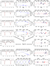 |
Fig. 1. Analysed systems and their fits. Each row of figures represents one system. The figures in the left column are the light curve fits from TESS data, while in the right column are the diagrams showing the period changes. Middle plots show the complete fit (apsidal motion plus LTTE), right-hand plots are only LTTE fits. Black dots indicate primary eclipses, blue dots are the secondary ones, while the red data show our newly dedicated observations. The bigger the symbol, the higher the weight and precision with which it was derived. |
3.2. ASASSN-V J052227.78+345257.6
Another ASAS-SN discovery was the star ASASSN-V J052227.78+345257.6, which has about 2.4-day period and was also not studied before. Just as with the previous star, we collected all the data available for our analysis. Thanks to the brightness of the star, there are much more older data, which helped us a lot in tracing the slow apsidal motion.
We used the TESS sector 59 for the modelling of the LC. The final parameters are given in Table 2. In the table, one can see that the level of the third light is significantly lower (it contributes only about 10% to the total light), and both components are much more detached than in the previous system. Quite surprisingly, we report an eccentricity of about 0.35, which is one of the highest values for the stars with periods below 2.5 days.
We were able to derive the times of eclipses from the data spanning back more than 20 yr. This is mainly due to the star’s rather deep eclipses. Five new eclipses were also observed with our telescopes especially for this study. Analysing all of these available data points resulted in the picture shown in Table 3 and Fig. 1. The apsidal motion has a period of about 450 yr, while the shorter ETV variation visible on both the primary and secondary eclipses has a periodicity of about 3.2 yr only. With the putative third body having such a short orbit, one can also ask whether some dynamical shorter-period perturbations would be detectable there on the human-life timescale. When computing the rough estimate of such effects (see e.g., Borkovits et al. 2016), the ratio of  gave us an order of magnitude estimation of the period of such a modulation. It resulted in about 1500 yr, which is short enough to be considered. For example, the most pronounced effect should be the precession of the orbital planes (i.e., a possible change of the eclipse depth of the inner eclipsing pair may be detectable during the next decades).
Parameters from the ETV analysis.
3.3. ASASSN-V J203158.98+410731.4
Next in our sample of stars is ASASSN-V J203158.98+410731.4, also known as RLP 961. It is probably the most studied system within our group of stars, partly due to its brightness. It was classified as a B1V star and a member of Cygnus OB2 association (Berlanas et al. 2018).
Our LC analysis was performed on the TESS light curve from sector 55. The results of the fitting are given in Table 2, and the fit is plotted in Fig. 1. As one can see, we interchanged the role of the two components (i.e., as the secondary component is more luminous, it has a larger radius and higher mass). This comes from the fact that we tried to place the deeper eclipse closer to the zero phase in the phased light curve. However, quite surprisingly, the additional third light value we found is in more than 50% of the total light.
We collected all available data for the period analysis. Apart from what came from TESS, the data included the observations from surveys ZTF, ASAS-SN, and SuperWASP. In addition, we also observed the star with our telescopes and derived five new times of eclipses, which follow the prediction quite well, as shown in Fig. 1. The apsidal motion resulted in a rather short apsidal period of about 52 yr. Additional variation has a period of 2.7 yr only. Due to its short outer orbit, the ratio  resulted in about 1030 yr, which is short enough to be detected in case of non-coplanar orbits (e.g., via an orbital precession), while the predicted angular separation of about 2 mas is too small to resolve an 11-mag star using current instruments.
3.4. ASASSN-V J230945.10+605349.3
The stellar system ASASSN-V J230945.10+605349.3 is probably the most interesting in our sample of stars. The never-before-studied star shows a detached-like LC with rather deep eclipses (the primary eclipse 0.4 mag deep), while its period is about 2.1 days. No spectral analysis was performed; however, even the low resolution Gaia spectra shows some weak indication of a double-peaked profile.
For the LC analysis, we used the TESS data from sector 58, which evidently shows a deeper primary but a wider secondary eclipse (see Fig. 1). Both eclipsing components are quite similar to each other (see Table 2), while the value of the third light only indicated a small fraction of the third light below 10%. The most surprising outcome in the analysis was the discovery of another variability on the TESS light curve (see Fig. 2). Very shallow additional eclipses were detected there (on all four sectors of data) having a period of 2.9925 days and a depth only about 1/30 of the of depth of the primary eclipses of pair A. Moreover, even shallower pulsational-like variability was visible on the B light curve, having a period of about 0.3 days. Very preliminary LC analysis of pair B indicated that its light contribution is really very small compared to the pair A (i.e., about 91% of the light comes from A and 9% from pair B). However, with only this statement, one cannot be sure that the two A and B binaries really constitute a bound quadruple system.
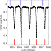 |
Fig. 2. Photometry of ASASSN-V J230945.10+605349.3 as obtained during sector 58 of TESS data. Deeper eclipses are from pair A (denoted with red abscissae), while shallower eclipses from pair B (blue abscissae) are only barely visible. |
A quite straightforward way to prove the gravitational coupling is an ETV analysis of both pairs. We used a method similar to the one in our recent publications detecting several new doubly eclipsing systems through ETV analysis of both pairs and ground-based photometric data from various surveys (see e.g., Zasche et al. 2023). The pair A shows an evident and quite rapid apsidal motion with a period of about 37 yr, and the eccentricity was derived to be 0.177. Figure 1 shows our final fit with the combination of apsidal motion and the LTTE hypothesis. However, for pair B, any such analysis was very difficult to reproduce. Pair B has only very shallow eclipses, and these cannot be detected in the ground-based data. Due to this, we only used the TESS data available from four sectors and plotted the times of eclipses of pair B to the ETV diagram of B below that of A with the same range of x-axis in order for them to be comparable. As one can see, there is evident variation of pair B’s eclipses in the anti-phase with respect to pair A’s eclipses, clearly showing that the star is a bound quadruple 2+2 stellar system. If one has adequately good data with times of eclipses for both the A and B pairs, one is in principle able to derive their ETV amplitudes and therefore also the mass ratio MA/MB of both pairs. However, the ETV here for pair B is so poorly constrained that the amplitude of variation of B could hardly be estimated. However, it does seem to be higher than for A, which is in agreement with the luminosity ratio of both A and B pairs.
3.5. ASASSN-V J231028.27+590841.8
The eclipsing system ASASSN-V J231028.27+590841.8 is the never-before-studied star. Its period is about 2.4 days, and it shows two rather incomparable eclipses. The primary one is narrow and about 0.12 mag deep, while the secondary eclipse is obviously longer in duration and less than half as deep as the primary one.
Due to a lack of temperature information from the Gaia DR3 (it is the faintest source in our sample of stars), we found it quite problematic to at least roughly estimate the temperature for the primary component for the LC modelling. Based on the photometric index Gaia DR3: (Bp − Rp) = 1.252 mag, we drew the conclusion (when ignoring the interstellar extinction) that the source is probably some dwarf star of the early K type. However, the index (J − H) from 2MASS (Skrutskie et al. 2006) is 0.275 mag, indicating a rather earlier type of early G star. On the other hand, the (B − V) index from APASS (Henden et al. 2015) is 0.869 mag, showing an early K star. This would be in good agreement with the previous estimate of Teff as 4853 K given by Gaia DR2 (Gaia Collaboration 2018).
Sector 57 was used for the LC modelling of the eclipsing pair. The results are given in Table 2, where one can see that the secondary component is also the more dominant one, both in temperature and radius (hence also in luminosity). A remarkably large fraction of the third light resulted from our LC modelling, suggesting a more massive third component in the system (there is no obvious close-by companion in the vicinity of the target that would contaminate the large TESS pixel). What is even more surprising here is the high value of eccentricity. With its 2.4-day period and e = 0.434, it is one of the record-breaking systems due to it having such a short orbital period.
Collecting the available data from various sources (ASAS-SN, ZTF, Atlas), we carried out a period analysis for the apsidal motion analysis. Its period of about 136 yr is still only poorly constrained with data. However, the short-period, additional variation in the ETV diagram (see Fig. 1) is now clearly visible, especially thanks to our dedicated observations. Luckily, one older observation was found (due to the proximity of the star to a known eccentric system PV Cas), which was obtained in Ondřejov observatory in 1994. Our data baseline was spread significantly by this one very useful data point. With two new observations, we arrived at a final picture of the whole system, presented in Fig. 1. The period of the ETV is about 4.9 yr, longest in our sample.
3.6. NSV 14698
The last system we studied was NSV 14698. It is the brightest star in our sample and has the longest orbital period, about 3.3 days. It was discovered as a variable by Romano (1958), and its spectral type was derived as B2 by Brodskaya (1953). However, no detailed analysis of the system has been published until now.
We took the TESS sector 58 for the LC analysis, resulting in the parameters given in Table 2 and the final plot in Fig. 1. As one can see, the two eclipsing components are rather similar to each other. This system exhibits the deepest eclipses among our sample of stars, which are caused by its large inclination angle being rather close to 90°. The third light value resulted in only a small fraction of the total light.
We collected all available data for the ETV analysis, which spans now more than 120 yr. Due in particular to the system’s deep eclipses, it was possible to derive many useful observations from photographic plate archives, such as DASCH (Tang et al. 2013). (For the complete analysis of all these data, see Fig. 1). As one can see from Fig. 1, several periods of the apsidal motion are covered (its period is about 54 yr). However, from the most recent data points with higher precision, another short-period and smaller-amplitude variation of LTTE can also be seen. We plotted only the more precise observations from TESS and our dedicated observations in the right-hand plot in Fig. 1. This small variation cannot be seen in older data due to its small amplitude (about 3 min only, which is the smallest LTTE amplitude in our sample) and due to its quite short orbital period (about half a year).
Such a short periodic variation is remarkable since most of the similar eccentric triple systems show much longer periods. Therefore, it would be expected to also take into account the dynamical effects of the third body in addition to the classical geometrical LTTE (similar to what was done in, e.g., Borkovits et al. 2015). However, due to its rather complicated fitting, we decided to use only the simplified LTTE approach while considering the limitations of such an approach. Our model therefore cannot provide realistic parameters. Rather, it is to be taken as proof that this star is really the most dynamically interacting in our sample and to possibly attract special attention to this system, both for observational as well as for modelling efforts. We computed that due to the low ratio of periods  (about only 28 yr), the ratio of amplitudes for both ETVs (LTTE and dynamical) result in about ALTTE/Aphys ≈ 0.027. This shows that the dynamical effect absolutely dominates here and that a more sophisticated approach for modelling is needed. We should also speculate about some possible inclination changes due to the third-body effects in the system. However, due to it having detectable eclipses during the whole 20th century, one can suspect that the system is probably close to co-planar and that these dynamical effects are small enough. However, what do not fit very well are the oldest data points from the first half of the 20th century. Having a very well-defined apsidal motion with the recent data from the last 20 yr, one would expect that the older observations would also be adequately well described with such an apsidal motion. However, one can see there is some small deviation of the older points. The most probable explanation for this discrepancy is the dynamical influence of the distant body and our inadequate fit.
4. Conclusions
We have carried out the very first analysis of six unstudied eclipsing eccentric systems with putative third bodies. These systems are of great importance to deepening our knowledge about the multiple systems, especially the dynamics of stellar triples. For this purpose, we plotted all known eclipsing systems showing some apsidal motion together with additional ETV variation interpreted as a third-body influence (see Fig. 3). Apart from the classical, well-known, and often studied systems (typically with GCVS names), we also plotted recent discoveries based on the new, precise TESS and Kepler data, which usually covers a much shorter time interval. Therefore, these systems typically show short periods for the third bodies, and the third components strongly and dynamically interact with the inner eclipsing pairs (see the green dots in Fig. 3. One can see that there is no obvious correlation between the inner and outer eccentricities. On the other hand, the system NSV 14698 is very ‘TESS-like’ compared to the other green points due to its short outer period.
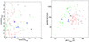 |
Fig. 3. Distribution of orbital parameters of currently known and published eccentric apsidal motion triples. The black dots denote well-known classical apsidal systems in our Galaxy; red dots are the stars in LMC/SMC; green dots denote new, recently published systems based on the new TESS and Kepler data; and the blue dots are the six new systems we present. |
What is probably the most interesting finding from our sample of new stars is the fact that a discovery of six new apsidal-motion triples can still be done with a modest technique and still on relatively bright stars. The brightest system in our sample (NSV 14698) has its magnitude below 11 mag, which is suitable for obtaining good spectra even with a moderate-sized telescope. Moreover, this system shows a fast apsidal motion together with a short ETV period, and it should be studied in detail due to its prospective complex dynamical behaviour. Therefore, we call for special attention on this star as well as for new observations, especially of this interesting target.
Acknowledgments
We would like to thank an anonymous referee for his/her useful suggestions greatly improving the whole manuscript. We do thank the NSVS, Kelt, ZTF, ASAS-SN, SWASP, and TESS teams for making all of the observations easily public available. The research of P.Z. and M.W. was partially supported by the project COOPERATIO – PHYSICS of the Charles University in Prague. This work has made use of data from the European Space Agency (ESA) mission Gaia (https://www.cosmos.esa.int/gaia), processed by the Gaia Data Processing and Analysis Consortium (DPAC, https://www.cosmos.esa.int/web/gaia/dpac/consortium). Funding for the DPAC has been provided by national institutions, in particular the institutions participating in the Gaia Multilateral Agreement. This research made use of Lightkurve, a Python package for TESS data analysis (Lightkurve Collaboration 2018). This research has made use of the SIMBAD and VIZIER databases, operated at CDS, Strasbourg, France and of NASA Astrophysics Data System Bibliographic Services.
References
- Aarseth, S. J., & Mardling, R. A. 2001, Evolution of Binary and Multiple Star Systems, 229, 77 [NASA ADS] [Google Scholar]
- Berlanas, S. R., Herrero, A., Comerón, F., et al. 2018, A&A, 612, A50 [NASA ADS] [CrossRef] [EDP Sciences] [Google Scholar]
- Borkovits, T. 2022, Galaxies, 10, 9 [NASA ADS] [CrossRef] [Google Scholar]
- Borkovits, T., Rappaport, S., Hajdu, T., et al. 2015, MNRAS, 448, 946 [NASA ADS] [CrossRef] [Google Scholar]
- Borkovits, T., Hajdu, T., Sztakovics, J., et al. 2016, MNRAS, 455, 4136 [Google Scholar]
- Borucki, W. J., Koch, D., Basri, G., et al. 2010, Science, 327, 977 [Google Scholar]
- Bozkurt, Z., & Deǧirmenci, Ö. L. 2007, MNRAS, 379, 370 [Google Scholar]
- Brodskaya, E. S. 1953, Izvestiya Ordena Trudovogo Krasnogo Znameni Krymskoj Astrofizicheskoj Observatorii, 10, 104 [NASA ADS] [Google Scholar]
- Claret, A. 2019, A&A, 628, A29 [NASA ADS] [CrossRef] [EDP Sciences] [Google Scholar]
- Claret, A., Giménez, A., Baroch, D., et al. 2021, A&A, 654, A17 [NASA ADS] [CrossRef] [EDP Sciences] [Google Scholar]
- Gaia Collaboration (Prusti, T., et al.) 2016, A&A, 595, A1 [NASA ADS] [CrossRef] [EDP Sciences] [Google Scholar]
- Gaia Collaboration (Brown, A. G. A., et al.) 2018, A&A, 616, A1 [NASA ADS] [CrossRef] [EDP Sciences] [Google Scholar]
- Gaia Collaboration (Vallenari, A., et al.) 2023, A&A, 674, A1 [NASA ADS] [CrossRef] [EDP Sciences] [Google Scholar]
- Heinze, A. N., Tonry, J. L., Denneau, L., et al. 2018, AJ, 156, 241 [Google Scholar]
- Henden, A. A., Levine, S., Terrell, D., et al. 2015, AAS Meet., 225, 336.16 [NASA ADS] [Google Scholar]
- Irwin, J. B. 1952, ApJ, 116, 211 [Google Scholar]
- Jayasinghe, T., Stanek, K. Z., Kochanek, C. S., et al. 2019, MNRAS, 486, 1907 [NASA ADS] [Google Scholar]
- Kim, C.-H., Kreiner, J. M., Zakrzewski, B., et al. 2018, ApJS, 235, 41 [Google Scholar]
- Kochanek, C. S., Shappee, B. J., Stanek, K. Z., et al. 2017, PASP, 129, 104502 [Google Scholar]
- Kozai, Y. 1962, AJ, 67, 591 [Google Scholar]
- Lidov, M. L. 1962, Planet. Space Sci., 9, 719 [Google Scholar]
- Lightkurve Collaboration (Cardoso, J. V. D. M., et al.) 2018, Astrophysics Source Code Library [record ascl:1812.013] [Google Scholar]
- Masci, F. J., Laher, R. R., Rusholme, B., et al. 2019, PASP, 131, 018003 [Google Scholar]
- Mayer, P. 1990, Bull. Astron. Inst. Czechoslovakia, 41, 231 [Google Scholar]
- Oelkers, R. J., Rodriguez, J. E., Stassun, K. G., et al. 2018, AJ, 155, 39 [Google Scholar]
- Pepper, J., Pogge, R. W., DePoy, D. L., et al. 2007, PASP, 119, 923 [NASA ADS] [CrossRef] [Google Scholar]
- Pollacco, D. L., Skillen, I., Collier Cameron, A., et al. 2006, PASP, 118, 1407 [NASA ADS] [CrossRef] [Google Scholar]
- Prša, A., & Zwitter, T. 2005, ApJ, 628, 426 [Google Scholar]
- Ricker, G. R., Winn, J. N., Vanderspek, R., et al. 2015, JATIS, 1, 014003 [Google Scholar]
- Romano, G. 1958, Mem. Soc. Astron. Ital., 29, 465 [NASA ADS] [Google Scholar]
- Shappee, B. J., Prieto, J. L., Grupe, D., et al. 2014, ApJ, 788, 48 [Google Scholar]
- Skrutskie, M. F., Cutri, R. M., Stiening, R., et al. 2006, AJ, 131, 1163 [NASA ADS] [CrossRef] [Google Scholar]
- Southworth, J. 2012, Orbital Couples: Pas de Deux in the Solar System and the Milky Way, 51 [Google Scholar]
- Tang, S., Grindlay, J., Los, E., et al. 2013, PASP, 125, 857 [NASA ADS] [CrossRef] [Google Scholar]
- Tokovinin, A. 2018, ApJS, 235, 6 [NASA ADS] [CrossRef] [Google Scholar]
- Udalski, A., Kubiak, M., & Szymanski, M. 1997, Acta Astron., 47, 319 [NASA ADS] [Google Scholar]
- Woźniak, P. R., Vestrand, W. T., Akerlof, C. W., et al. 2004, AJ, 127, 2436 [Google Scholar]
- Zasche, P., Wolf, M., Vraštil, J., et al. 2014, A&A, 572, A71 [NASA ADS] [CrossRef] [EDP Sciences] [Google Scholar]
- Zasche, P., Henzl, Z., Mašek, M., et al. 2023, A&A, 675, A113 [NASA ADS] [CrossRef] [EDP Sciences] [Google Scholar]
All Tables
All Figures
|
Fig. 1. Analysed systems and their fits. Each row of figures represents one system. The figures in the left column are the light curve fits from TESS data, while in the right column are the diagrams showing the period changes. Middle plots show the complete fit (apsidal motion plus LTTE), right-hand plots are only LTTE fits. Black dots indicate primary eclipses, blue dots are the secondary ones, while the red data show our newly dedicated observations. The bigger the symbol, the higher the weight and precision with which it was derived. |
| In the text | |
|
Fig. 2. Photometry of ASASSN-V J230945.10+605349.3 as obtained during sector 58 of TESS data. Deeper eclipses are from pair A (denoted with red abscissae), while shallower eclipses from pair B (blue abscissae) are only barely visible. |
| In the text | |
|
Fig. 3. Distribution of orbital parameters of currently known and published eccentric apsidal motion triples. The black dots denote well-known classical apsidal systems in our Galaxy; red dots are the stars in LMC/SMC; green dots denote new, recently published systems based on the new TESS and Kepler data; and the blue dots are the six new systems we present. |
| In the text | |
Current usage metrics show cumulative count of Article Views (full-text article views including HTML views, PDF and ePub downloads, according to the available data) and Abstracts Views on Vision4Press platform.
Data correspond to usage on the plateform after 2015. The current usage metrics is available 48-96 hours after online publication and is updated daily on week days.
Initial download of the metrics may take a while.