| Issue |
A&A
Volume 685, May 2024
|
|
|---|---|---|
| Article Number | A4 | |
| Number of page(s) | 12 | |
| Section | Extragalactic astronomy | |
| DOI | https://doi.org/10.1051/0004-6361/202348864 | |
| Published online | 30 April 2024 | |
The different flavors of extragalactic jets: Magnetized relativistic flows
1
INAF/Osservatorio Astrofisico di Torino, via Osservatorio 20, 10025 Pino Torinese, Italy
e-mail: This email address is being protected from spambots. You need JavaScript enabled to view it.
2
Dipartimento di Fisica, Università degli Studi di Torino, via Pietro Giuria 1, 10125 Torino, Italy
Received:
6
December
2023
Accepted:
27
January
2024
Abstract
We performed three-dimensional numerical simulations of magnetized relativistic jets propagating in a uniform density environment in order to study the effect of the entrainment and the consequent deceleration, extending a previous work in which magnetic effects were not present. As in previous papers, our aim is to understand the connection between the jet properties and the resulting Fanaroff-Riley classification. We considered jets with different low densities, and therefore low power, and different magnetizations. We find that lower magnetization jets effectively decelerate to sub-relativistic velocities and may then result in an FR I morphology on larger scales. Conversely, in the higher magnetization cases, the entrainment and consequent deceleration are substantially reduced.
Key words: magnetohydrodynamics (MHD) / methods: numerical / galaxies: jets
© The Authors 2024
 Open Access article, published by EDP Sciences, under the terms of the Creative Commons Attribution License (https://creativecommons.org/licenses/by/4.0), which permits unrestricted use, distribution, and reproduction in any medium, provided the original work is properly cited.
This article is published in open access under the Subscribe to Open model. This email address is being protected from spambots. You need JavaScript enabled to view it. to support open access publication.
1. Introduction
The traditional Fanaroff-Riley classification (Fanaroff & Riley 1974) divides extragalactic radio sources into two groups, it is based on morphological properties, but it is also reflected in radio luminosity. Fanaroff-Riley I (FR I) are low radio power sources and are characterized by jet-dominated emission that smoothly extends into the intracluster medium, where large-scale plumes or tails of diffused emission are observed. The second class, Fanaroff-Riley II (FR II), is characterized by higher radio power and the sources in this class show the maximum brightness in the hot spots at the jet termination. Recently a third class of radio-galaxies was introduced, representing the majority of the local radio-loud Active Galactic Nuclei (AGN) population. Because they lack the prominent extended radio structure characteristic of the other Fanaroff-Riley classes they were called FR 0 (Baldi & Capetti 2009, 2010; Sadler et al. 2014; Baldi et al. 2015). There is, however, a minority of FR 0 sources that show evidence of small-scale jets, usually limited to sizes of a few kiloparsecs (Baldi et al. 2019). This suggests that jets in this class are not even able to escape from the galaxy core. There is observational evidence that, both in FR I and in FR II, the jets at their base (at the parsec scale) are relativistic, with similar Lorentz factors (Giovannini et al. 2001; Celotti & Ghisellini 2008). The situation is less clear for FR 0 sources: Giovannini et al. (2023), from VLBI observations, conclude that jets in FR 0 can be, at most, mildly relativistic. However, Massaro et al. (2020) suggest that FR 0 could represent the misaligned counterpart of a significant fraction of BL Lac objects and therefore they should also be associated with relativistic jets. This apparent contradiction could be solved by considering a jet with a transverse velocity structure, with a relativistic spine surrounded by a non-relativistic flow. It is clear that in FR I jets, and possibly in FR 0 jets, a deceleration to sub-relativistic velocities must occur between the inner region (at the parsec scale) and the kiloparsec scale, where FR Is show their plume-like morphology (Laing & Bridle 2002a, 2014) and FR 0s disappear. Massaglia et al. (2016) performed high-resolution three-dimensional simulations of low Mach number jets, showing the onset of turbulence and the formation of structures very similar to that observed in FR I sources (see also van der Westhuizen et al. 2019). However, in this study, the jets are injected already at non-relativistic velocities and one has to assume that deceleration has already occurred.
Deceleration occurs most likely through the progressive turbulent entrainment of external material (see e.g. De Young 1993, 2005; Bicknell 1984, 1986, 1994; Wang et al. 2009) as a consequence of the development of jet instabilities, in particular Kelvin-Helmholtz (see e.g. Perucho & Martí 2007; Rossi et al. 2008, 2020), among others. The role of current-driven instabilities has been considered, for example, by Tchekhovskoy & Bromberg (2016), Massaglia et al. (2019, 2022) and Mukherjee et al. (2020). Moreover, it was recently pointed out that recollimation shocks may trigger instabilities and possible entrainment; in particular, Gourgouliatos & Komissarov (2018a,b) and Abolmasov & Bromberg (2023), discuss the development of the relativistic centrifugal instabilities, and Costa et al. (in prep.) consider Kelvin-Helmholtz instabilities. We must also mention a second option, which may be complementary to turbulent entrainment, related to mass loading by stellar mass loss (Komissarov 1994; Bowman et al. 1996; Laing & Bridle 2002b; Perucho 2014, 2020; Perucho et al. 2014; Anglés-Castillo et al. 2021).
In this paper we extend the work by Rossi et al. (2008) and Rossi et al. (2020, hereafter Paper I and Paper II). They performed numerical simulations of the propagation of relativistic unmagnetized jets, with different density ratios between the jet and the ambient medium, studying the entrainment and deceleration process in detail. They found that lighter jets are more prone to deceleration. In particular, in Paper II, we followed the jet propagation up to a distance of about 600 initial jet radii, showing how jets, with a density ratio of 10−4, are able to reach a quasi-steady configuration, where the Lorentz factor decreases from 10, at the injection point, to about 2, close to the jet head. On the contrary, denser jets can propagate in an almost undisturbed way. The main limitation of the analyses presented in Papers I and II is the absence of magnetic field; our aim in the present work is to overcome this limitation.
In this paper, we concentrate our analysis on the role of the density ratio and of the field strength in determining the jet deceleration process and we will show that these parameters play a very important role in this process. Of course, there are also other aspects that are likely to play a relevant role in the jet stability and evolution, such as i) different magnetic field configurations, ii) different initial Lorentz factors, iii) inhomogeneities in the ambient medium. However the parameter space is very wide and one has to proceed in a step-by-step manner.
In Sect. 2 we describe the set of equations to be solved, the numerical method, the initial and boundary conditions and the parameters of the simulations. In Sect. 3 we present our results and in Sect. 4 we give discussion and conclusions.
2. Numerical setup
Numerical simulations are carried out by solving the equations of relativistic ideal magneto-hydrodynamics in 3D. They are expressed by
 (1)
(1)
![Mathematical equation: $$ \begin{aligned}&\partial _t \left( \gamma ^2 \rho h \mathbf v + \mathbf E \times \mathbf B \right) \nonumber \\&\qquad \qquad + \nabla \cdot \left[] \gamma ^2 \rho h \mathbf v \mathbf v - \mathbf E \mathbf E - \mathbf B \mathbf B + \left( p + u_{em}\right) \mathbf I \right] = 0 , \end{aligned} $$](/articles/aa/full_html/2024/05/aa48864-23/aa48864-23-eq2.gif) (2)
(2)
 (3)
(3)
 (4)
(4)
where the electric field E is provided by the ideal condition E + v × B = 0. In this set of equations, ρ is the proper density, v is the velocity three-vector (in units of the light speed c), B is the laboratory magnetic field (in units of  ),
),  is the Lorentz factor, h is the relativistic specific enthalpy, uem = (E2 + B2)/2, and I is the unit 3 × 3 tensor. The system of Eqs. (1)–(4) is completed by specifying an equation of state relating h, p, and ρ. Following Mignone et al. (2005), we adopted the Taub-Mathews (TM) equation of state, with the prescription
 (5)
(5)
which closely reproduces the thermodynamics of a Synge gas for a single species relativistic perfect fluid (notice that we set c = 1, since the light speed is our unit of velocity).
In addition to the system (1)–(4), we also integrate the equation
 (6)
(6)
which describes the evolution of a passive tracer f, set to unity for the injected jet material and to zero for the ambient medium. This way, we can follow the evolution of the spatial distribution of the jet material and its mixing with the ambient medium.
Simulations were carried out in a Cartesian domain with coordinates in the following range: x ∈ [−Lx/2,Lx/2], y ∈ [0,Ly] and z ∈ [−Lz/2,Lz/2]. At t = 0 the domain is filled with a perfect fluid of uniform density and pressure, representing the external medium initially at rest. In addition, we assume the external medium to be initially unmagnetized. The assumption of constant density is consistent with the fact that we focus on the jet propagation inside the galaxy core.
A cylindrical inflow of velocity vj, proper density ρj, and a purely azimuthal magnetic field is constantly fed into the domain at y = 0, along the y direction. The jet is characterized by its radius rj, the Lorentz factor γj, the ratio ηj between its proper density ρj, and the external density and the Mach number defined as Mj = vj/cs0, where cs0 is the sound speed on the jet axis. The sound speed cs0 is given by the expression valid for the TM equation of state (Mignone et al. 2005):
 (7)
(7)
where p0 and h0 are, respectively, the pressure and the specific enthalpy computed on the jet axis. The specific enthalpy can be derived through Eq. (5). The injected magnetic field has a configuration corresponding to a constant current density inside r = a (we take a = 0.75rj) and zero outside:
 (8)
(8)
where Bm is the maximum magnetic field strength reached at r = a. The return current during the jet evolution follows the backflow and the shocked ambient medium similarly to what is seen in Leismann et al. (2005). Inside the jet (r < rj), we assume total pressure equilibrium, therefore the thermal pressure inside the jet is given by
 (9)
(9)
The value of p0, as discussed above, is related to the jet Mach number Mj, while the value of Bm, in the jet rest frame, can be obtained through the magnetization parameter  . The external medium can be characterized by the parameter
 (10)
(10)
where pa and ρa are, respectively, the pressure and density of the external medium.
The equations are non-dimensionalized by using c as the unit of velocity (as already discussed), the jet radius rj as the unit of length and the ambient density ρa as the unit of density. To specify completely the problem, we therefore need the following non-dimensional parameters (introduced above): the jet Lorentz factor γj, the density ratio ηj, the jet Mach number Mj, the jet magnetization σj, and the non-dimensional ambient pressure Π. In our analysis we kept the Lorentz factor γj = 10, the Mach number Mj = 2.2, and Π = 5 × 10⁻⁷ (corresponding to a temperature of the ambient medium of 5 × 10⁶ K) fixed. We instead varied the density ratio ηj and the magnetization σj for a total of four simulations. All the jets result to be over-pressured with respect to the ambient medium. The parameters of the simulations are reported in Table 1, where we also report the pressure contrast K between the jet and the ambient, the relativistic specific enthalpy in the jet and the jet power discussed below.
Parameter set used in the numerical simulation model.
Numerical integration of the system (1)–(4) is performed using the ideal relativistic magnetohydrodynamics module in the PLUTO code (Mignone et al. 2007). For the present application we employed linear reconstruction, second-order Runge-Kutta time stepping, and the HLLD Riemann solver (Mignone et al. 2009). Constrained transport (Balsara & Spicer 1999; Londrillo & del Zanna 2004) is used to maintain the condition ∇ ⋅ B = 0. For the physical domain extension we choose Lx = 300, Ly = 600, and Lz = 300 and we cover this domain with a grid of 350 × 2400 × 350 grid points, which are uniformly spaced in the region around the jet axis (−15 < x < 15, −15 < z < 15) and geometrically stretched outside. The cells are elongated in the jet directions and we have a resolution of 8 points on the jet radius in the x and z directions and of 4 points on the jet radius in the y direction. The boundary conditions are outflow on all the boundaries except for y = 0, where, for r < rj we have inflow conditions and, for r > rj we have reflective conditions.
3. Results
Our aim is to understand how the deceleration process occurs as a function of the density contrast and the jet magnetization. We then take two values for the density contrast, η = 10−4 and 10−5, and two values for the jet magnetization, σj = 10−2 and 10−1, as shown in Table 1. In principle the setup of our simulations is scale invariant; however, our interest is focused on the deceleration that mainly occurs in the first kiloparsec. This motivates our assumption of constant density of the external medium because the domain of our simulations can be assumed to be all contained within the galaxy core. We can then adopt, as in Paper I, a jet injection radius on the order of one parsec and the external density at injection on the order of one particle per cubic centimeter (Balmaverde & Capetti 2006). In the following, we express all quantities in their non-dimensional values as defined in the previous section. Conversion to physical units can be obtained with the above assumptions; in particular, the unit of time is
 (11)
(11)
and the jet power is
 (12)
(12)
where h0 is the relativistic specific enthalpy, defined in Eq. (5) and n0 is the external number density. With the assumption of the jet Mach number Mj = 2.2, the value of h0 is 1.6. The jet power for the four cases is reported in Table 1. We choose the parameters so that the resulting powers are at about the dividing power between FR I and FR II.
We followed the jet propagation for Cases A and B until the bow shock in front reached y = 600; in Cases C and D we stopped the simulations somewhat earlier because in these cases the cocoon edge reached the lateral boundaries. In these cases, the jet head at the end of the simulation reaches y ∼ 550.
3.1. Jet dynamics
In the two panels of Fig. 1, we show the jet-head position as a function of time for all the cases; more precisely, the top panel shows Cases A and B, with the density ratio ηj = 10−4, and the bottom panel shows Cases C and D, with the density ratio ηj = 10−5. The dashed black line in each panel shows the estimated head position obtained by using the theoretical value of the jet-head velocity, in the relativistic case, given by Martí et al. (1997) (see also Bromberg et al. 2011). This value has been obtained, by equating the (relativistic) momentum flux of the jet and the ambient medium, as
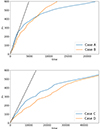 |
Fig. 1. Position of jet head as a function of time; the top panel shows Cases A and B and the bottom panel shows Cases C and D. |
 (13)
(13)
where h0 and ha are, respectively, the specific relativistic enthalpies of the jet and of the ambient. In the top panel, we see that Case A (blue curve, lower magnetization σj = 0.01) follows the theoretical estimate closely up to yh ∼ 300 (t ∼ 2500). Actually the jet-head velocity reaches values that are slightly higher than the theoretical estimate and this could be interpreted as the result of jet-head wobbling as in Aloy et al. (1999) and Perucho et al. (2019). After this initial phase, we observe a strong deceleration. In Case B (orange curve, higher magnetization σj = 0.1), at the beginning, the jet head appears to advance more slowly than in Case A; however, the deceleration is much less efficient, and the jet head reaches the end of the domain in about half the time with respect to Case A (t ∼ 12 000 for Case B vs. t ∼ 23 000 for Case B). In the bottom panel, Cases C and D propagate at a much lower velocity, as is expected from the lower density ratio. Case C, with lower magnetization (σj = 0.01, blue curve), at the beginning, propagates faster than Case D (orange curve, higher magnetization σj = 0.1), but, at later times, Case C shows a stronger deceleration, and the two cases reach the end of the domain at similar times (t ∼ 45 000).
From Fig. 2, we obtain an impression of the final structure of the jets. In the figure, we show the 3D distribution of the Lorentz factor for all the cases, when the jet reached its maximum length. The four snapshots correspond to four different times; namely t ∼ 23 000 for Case A, t ∼ 12 000 for Case B, t ∼ 42 000 for Case C and t ∼ 48 000 for Case D. The differences in times are due to the different jet-head propagation velocities, as shown above. In the figures, we display 3D views of the isocontours for three values of the Lorentz gamma factor (γ = 1.1, 3, 5). Each panel shows both the entire jet and a zoomed-in view of the last 200 length units. The represented domain, in the transverse direction, extends from −30 to 30, in both directions, for all cases except Case A, which extends from −40 to 40, since in this case we observe a larger expansion of the jet. In Cases A and C, which are less magnetized, we have a behavior similar to that of the hydrodynamic cases discussed in Paper II. We observe a first region, in which the jet seems to propagate straight, and then (for y ≳ 100 in Case A and y ≳ 250 in Case C) we observe the growth of perturbations, with the appearance of jet wiggling, and eventually the jet breaks into small high-velocity fragments surrounded by slowly moving material. We note that we do not add any perturbation at the jet inlet and the growth of perturbations is solely due to the jet-backflow interaction. In Case A, the zoomed-in view of the last part of the jet shows that material moving at γ > 5 is practically absent. The behavior of the more magnetized cases (B and D in the right panels) is quite different. The high velocity part of the jet remains more coherent, with some wiggling, but at a larger scale with respect to the other two cases. The jet fragmentation occurs, but the high velocity fragments are larger and are present up to the jet head.
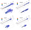 |
Fig. 2. Three-dimensional isosurfaces of Lorentz factor at the end of the simulations. The top left panel represents Case A at t = 23 000, the top right panel represents Case B at t = 12 000, the bottom left panel represents Case C at t = 42 000, and finally, the bottom right panel represents Case D at t = 48 000. In each panel the top portions display the entire jet while the bottom portions display the last section of the jet between y = 400 and y = 600. The three isosurfaces are for γ = 1.1, 3, 5. |
The behavior described above can be better appreciated in Fig. 3, where we display a longitudinal cut (in the y − z plane) of the distribution of the Lorentz factor at the final times of the simulations. In Paper II we described three regions along the jet characterized by a different jet behavior. In the first region the jet propagates almost undisturbed and we observe the presence of several recollimation shocks, in the second region perturbations grow until, in the last region, the jet is broken into a few fast-moving blobs surrounded by a wide low-velocity envelope. In the present simulations, these regions are clearly visible for Cases A and C. In Case A, the unperturbed region is quite short, up to y ∼ 100, and it is characterized by strong recollimation shocks. The second region spans the jet length from y ∼ 100 to y ∼ 250 and for y ≳ 250 the jet is fragmented. In case C, the first region ends at y ∼ 250, and the recollimation shocks are quite weak; the second region ends at y ∼ 350, and the fragmentation region is observed for y ≳ 350. A comparison with the results of Paper II (see Case C of Paper II with a density ratio of 10−4) shows that in Case A we have a much faster growth of perturbations and an earlier jet fragmentation, while Case C behaves similarly to the hydro case. We can also notice that, in Case A, the entrainment region is much wider with respect to case C (and the hydro cases). Cases B and D, which are more magnetized, show a quite different behavior, the jet propagates quite straight for larger distances, up to y ≳ 300 and then appears to break more suddenly, with the formation of larger fragments and a much lower entrainment.
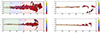 |
Fig. 3. Longitudinal cut (in the y − z plane) of Lorentz factor distribution at final simulation times. The four panels refer to the four different cases (Case A: top left; Case B: top right; Case C: bottom left; Case D: bottom right). The times are the same as in Fig. 2. The three colored bands in the left panels (Cases A and C) highlight the three phases described in the text. |
3.2. Jet entrainment and momentum transfer
The results presented above show that, in Cases A and C, the jet progressively decelerates and the quantity of material moving at high γ decreases, while an increasing amount of material around the jet moves at γ ≤ 2. We can more quantitatively analyze how the entrainment and deceleration processes occur. In Fig. 4 we show the behavior of the entrained mass as a function of jet-head position; more precisely, we define the entrained mass as the total mass of the external material moving with vy > 0.1. The four curves in the figure refer to the four different cases. Case A, as expected, is the one with the highest value of the entrained mass. Most of the entrainment occurs for 400 < yh < 600, which corresponds to 7000 < t < 24 000, that is, to the largest fraction of the duration of the jet evolution. For Case C, we had to stop the simulation somewhat earlier with respect to Case A because the lateral bottom part of the cocoon leaves the computational grid. Up to this point, however, Case C behaves similarly to Case A. For the more magnetized Cases B and D, instead, the entrained mass is much lower, less than 10% of that of Case A.
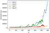 |
Fig. 4. Plot of entrained mass as a function of jet-head position for all the cases. The entrained mass is defined as the mass of the external material moving at vy > 0.1. |
In the entrainment process, the jet transfers its momentum to the external medium. A quantitative view of this process is provided by Fig. 5, in which we plot, as a function of time, the maximum distance at which a given fraction of the momentum flux is carried by material moving at γ ≥ 5. We start our discussion by looking at the top left panel, corresponding to Case A. In the figure we see several curves: starting from the top, the blue curve represents the head position, the region between the top curve and the second curve refers to a jet section in which the high-velocity material carries a fraction of momentum flux < 10%; the second region refers to a fraction 10%−20% and so on; the bottom curve refers to a fraction of 70%. Up to t ∼ 3000, all the curves follow the behavior of the jet head; subsequently, all the curves tend to flatten and for t ≳ 8000 they become flat on average. As discussed in Paper II, the flattening shows that the jet has reached a quasi-steady state in which it progressively entrains external material and slows down. We can see that, in this quasi-steady state, the jet up to y ∼ 250 propagates almost undisturbed, with the high velocity material carrying most of its momentum; in the 250 ⪅ y ⪅ 400 region, the jet progressively transfers its momentum to the entrained external material, the momentum fraction carried by the high velocity material drops from 70% to < 10%, and, finally, in the y > 400 region almost all the initial jet momentum is carried by slow moving material. We can notice that, as discussed above, the region between y ∼ 250 and y ∼ 400 corresponds to the region where the perturbations progressively increase their amplitude until the jet becomes fragmented. In the bottom left panel, we show the results for Case C, which has a density contrast of η = 10−5 and the same magnetization, σ = 10−2, as Case A. In this case, a quasi-steady state is almost reached, and all the curves tend to flatten, but, on average, they are still increasing. The process of entrainment and deceleration occurs at a greater distance with respect to Case A, that is, from y ∼ 350 to y ∼ 450, and can be connected, as in Case A, with the growth of perturbations and jet fragmentation that is observed in Fig. 3.
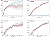 |
Fig. 5. Maximum distance from the jet origin at which a given fraction of momentum flux is carried by material moving at γ ≥ 5 as a function of time. The four panels refer to the four different cases (Case A: top left; Case B: top right; Case C; bottom left; Case D: bottom right). In each panel the top curve shows the jet head position and the other curves represent the fractions from 10% to 70%. For Cases A and C we highlight the areas between subsequent curves with different colors. |
In Cases C and D, which have higher magnetization (σ = 0.1), the behavior is quite different. We already saw that the entrainment process is much less efficient with respect to the other two cases and therefore the jet does not lose its momentum almost up to its head. Without entrainment and transfer of momentum to the external material we would not observe any deceleration and, in this case, we would expect all the curves to be coincident with the jet propagation. This is confirmed by the behavior of the different curves in the right panels of Fig. 5 (top, Case B, η = 10−4; bottom, Case D, η = 10−5), which closely follow the blue line representing the position of the jet head.
Combining the information presented above, we derived a different scenario for the low-magnetization Cases A and C with respect to the high-magnetization Cases B and D. In Cases A and C, the jet is subject to Kelvin-Helmholtz instability, which drives turbulent entrainment, and progressively releases its momentum into the ambient medium; it widens its cross-section, maintaining a high gamma value only in a central spine until it breaks and fragments into high-velocity blobs, surrounded by an envelope at γ ≤ 2. In Case A, however, this process is more efficient and, in the last section of the jet, the high-velocity material is almost absent. In Case C, the process is less efficient it occurs later and fragments of high-velocity material are often present in the last section of the jet, as we show later. The Cases B and D, with higher magnetization, appear to be less prone to Kelvin-Helmholtz instabilities, but the jet presents larger scale wiggles that are most likely due to current-driven instabilities. These differences between low- and high-magnetization cases were already discussed by Mignone et al. (2010), Massaglia et al. (2019, 2022), and Mukherjee et al. (2020). These papers showed how the larger toroidal magnetic fields stabilize the jet against short-wavelength Kelvin-Helmholtz modes that are responsible for the turbulent entrainment, but that lead to current-driven instabilities that result in larger scale jet wiggling (see also López-Miralles et al. 2022), the formation of larger scale fragments, and a lower efficiency of entrainment. The development of current-driven instability is of course enhanced by the presence of only the azimuthal component of magnetic field. In a more general field configuration, the behavior can be somewhat different.
3.3. Jet deceleration
The entrainment process discussed above may lead to different connected consequences for the jet dynamics. First, we can have a decrease in the strength of the terminal shock up to its disappearance. In Massaglia et al. (2016) the authors interpret this disappearance as a signature of the transition from FR II to FR I; in fact the presence of a strong terminal shock can be connected with the presence of hot spots typical of FR II radio sources. As a second point, the Lorentz factor in the terminal part of the jet, that is, in the region close to its head, may tend to decrease, and, finally, the jet-head velocity also decreases. In Figs. 6–9 we give representations of these different aspects for the four different cases. More precisely, in the top left panel of each figure we show a scatter plot of the maximum pressure in the computational domain, as a function of time (bottom x-axis) and jet head position (top x-axis); the colored band highlights the range of variation and the general trend. In the top right panel, we plot the y position of the maximum pressure, again as a function of time (bottom x-axis) and jet head position (top x-axis). In the bottom left panel we plot the maximum value of the Lorentz γ near the jet head as a function of time (bottom x-axis) and jet head position (top x-axis). More precisely, in the figure, we plot the maximum value of γ found in the yh − 50 < y < yh region, where yh is the y coordinate of the position of the jet head. Finally, in the bottom right panel we show the velocity of the jet head again as a function of time (lower axis) and of the head position (upper axis).
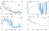 |
Fig. 6. Four different plots describing different aspects of the jet dynamical behavior for Case A. Top left panel: maximum pressure found in the computational domain as a function of time (bottom axis) and the position reached by the jet head (top axis). The symbols mark the values for each time, while the colored band identifies the range of variation. Top right panel: plot of y coordinate of maximum pressure, plotted in the top left panel, as a function of time (bottom axis) and the position reached by the jet head (top axis). Bottom left panel: plot of maximum Lorentz factor near the jet head as a function of time (bottom axis) and position reached by the jet head (top axis). More precisely, the maximum value of γ is in the region yh − 50 < y < yh, where yh is the jet-head position. Bottom right panel: plot of jet-head velocity as a function of time (bottom axis) and position reached by the jet head (top axis). |
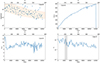 |
Fig. 7. Same as Fig. 7, but for Case B. The two vertical black lines in the bottom right panel indicate one of the time intervals in which the jet slows down because of the bending of the jet head as shown in Fig. 10. |
For Case A (Fig. 6), in the top left panel, we can observe the presence of two phases; at first the maximum pressure shows a decreasing trend followed by a flatter behavior, which starts at t ≳ 104, when the jet head has reached y ∼ 500. In the flat part, the maximum pressure typically remains at a low level, with some sporadic spikes. Correspondingly, in the top right panel we observe that, up to t ∼ 104 and yh ∼ 500, the maximum pressure is found at the jet head, while for longer times, there are intervals in which the maximum pressure is observed in the first section of the jet. This indicates that the terminal shock has disappeared and thus the jet has acquired a morphology more similar to an FR I. We can notice that the time at which there is the occurrence of the transition between the two phases corresponds to the time at which we observe, in the top left panel, the transition to a quasi-steady state. The same two phases can also be observed in the bottom panels. In the bottom left panel, we can see that for t < 12 000 (yh < 500) on average the maximum value of γ is around 8, on average. For longer times, t > 12 000 (yh > 500), it drops abruptly to a value of about 2, with some isolated peaks that are anyway < 4, except in very few instances. The jet deceleration is confirmed by the bottom right panel, where we observe, in the first phase, strong oscillations of the jet head velocity. A smoother behavior is instead present in the second phase. As discussed earlier, the time of transition between the two phases corresponds to the time at which the jet reaches a quasi-steady state. Overall, in Case A, which shows the more pronounced effects of entrainment, the jet-head velocity decreases from the beginning to the end by a factor slightly larger than 10.
For Case C (Fig. 8), in the top left panel we similarly observe a two-phase behavior; in the first phase, up to t ∼ 25 000 and yh ∼ 420, we observe a steady decrease, followed again by a flatter part. The range of variation is, however, larger than in Case A and high pressure peaks occur much more frequently. Correspondingly, in the top right panel of Fig. 8, we observe that the intervals in which the terminal shock disappears are very sporadic, and therefore the jet almost always has a FR II-like morphology. Again the transition between the two phases occurs at the time when the jet has almost reached a steady state. Similarly, in the bottom left panel we observe that for t < 25 000 (yh < 400) the average value of γ is again around 8, at larger times it shows strong oscillations with an average value of around 4, but these drops quite often to values of around 2. Also, the behavior of the jet-head velocity is similar to Case A, with somewhat larger oscillations in the second phase. In fact, as discussed above, in the quasi steady state, we have more high velocity fragments that reach the jet head and this leads to the observed sporadic increases of the jet-head velocity. The velocity decrease is somewhat lower than in Case A.
For the more magnetized Cases B and D (Figs. 7 and 9), in the top left panels we do not observe the two-phase behavior, but only a decreasing trend with a quite large interval of variation and the values of the maximum pressure remains typically higher than in Cases A and C. The position of the maximum pressure, shown in the top right panels, is always at the jet head (with only very few exceptions for Case D) and the maximum values of γ stay, for all times, around 8, with some sporadic drops at lower values, particularly for Case D. The jet-head velocity, in the bottom right panels, shows a strongly oscillating behavior for all times. The oscillations can be connected to the swirlings of the jet head induced by the current-driven kink instability. This is demonstrated by Fig. 10, where we show a sequence of 3D views of a tracer iso-contour during the interval of time marked by the two black vertical lines in the bottom right panel of Fig. 7 (Case B). We can see that, in correspondence to the decrease of the jet-head velocity, the jet head is deflected at almost 90 degrees and then the jet returns to propagate straight and the velocity to increase again. Overall, as a result of the lower efficiency of the entrainment process, the jet-head velocity for these cases decreases less with respect to the previous ones.
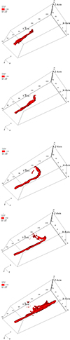 |
Fig. 10. 3D iso-contours of the tracer (for a tracer value of 0.7), for Case B, at five different times in the interval marked by the black vertical lines in the top right panel of Fig. 7. |
The structure of the magnetic field appears also quite different between low and high magnetization cases, as shown in Fig. 11, where we display longitudinal cuts, in the y − z plane, of the distribution of the magnetic field intensity. In the two left panels, corresponding to the low magnetization cases, we can see that for y ≥ 300 the magnetic field is characterized by small-scale structures. This occurs in the region where turbulent entrainment is most effective. On the contrary, higher magnetization cases in the right panels show a much more coherent structure of the magnetic field concentrated along the jet for almost all its length. This is consistent with the results of Mukherjee et al. (2020), where similar differences in the magnetic field distribution are found between the cases dominated by the Kelvin-Helmholtz instability (as our Cases A and C) and the cases dominated by the current-driven kink instability (as our Cases B and D).
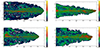 |
Fig. 11. Longitudinal cut (in the y − z plane) of the distribution of the magnetic field strength at the final times of the simulations. The four panels refer to the four different cases (Case A top-left, Case B top-right, Case C bottom-left, Case D bottom-right). The times are the same as in Fig. 2. |
4. Summary and conclusions
We presented 3D simulations of relativistic magnetized jets, considering four cases with the same Lorentz factor γ = 10, but different density ratios and different magnetization, with the aim of studying the deceleration process in connection with the FR I-FR II dichotomy. We follow the propagation up to about 600 pc within the galaxy core, so our assumption of constant density is well justified. Since in FR I radio sources the jets are relativistic at their base, but they become sub-relativistic farther out, our simulations are aimed, as in Papers I and II, at investigating under which conditions highly relativistic collimated flows can decelerate to sub-relativistic velocities within a distance of about one kiloparsec. Here we extend the analysis performed in Papers I and II, by considering the effects of magnetic field.
Different kinds of instabilities may play a role in shaping the dynamics during the jet propagation; in particular, the Kelvin-Helmholtz instability, as shown in Papers I and II, can lead to mixing, transfer of momentum and then jet deceleration. The presence of magnetic field, on the other hand, may have a strong impact on the instability evolution; in fact, it can stabilize the jet against Kelvin-Helmholtz instabilities, but it can promote the growth of current-driven instabilities, leading to strong jet bendings and deflections (see e.g. Mignone et al. 2010).
In Papers I and II we showed how lighter jets are more prone to deceleration. In particular the most promising case was Case C of that paper, which had a density ratio η = 10−4. In the present paper we then consider cases with parameters similar to those of Case C, with η = 10−4. In addidition, we also considered cases with a lower density ratio (η = 10−5). For both values of the density ratios we considered different magnetization. Our results show striking differences between low- and high-magnetization cases. While the low-magnetization cases (A and C) show the effects of entrainment and momentum transfer to the external medium, in high-magnetization cases (B and D) entrainment and momentum transfer appear to be much less efficient. As discussed above, this difference is due to the magnetic field that has a stabilizing effect on Kelvin-Helmholtz instabilities and reduces the mixing. On the other hand, stronger magnetic fields can drive current-driven instabilities, and, in fact, in Cases B and D we observe larger scale wigglings and jet bending. Comparing Cases A and C, we can observe that in Case C the entrainment process is somewhat less efficient than in Case A and it starts at a more advanced position along the jet. The start of entrainment in Case A appears to be connected with the presence of strong recollimation shock at the jet base. The presence of recollimation shocks can favor the growth of instabilities (Costa et al., in prep.; Abolmasov & Bromberg 2023; Gourgouliatos & Komissarov 2018a,b); in fact, after the shock both the Lorentz factor and the Mach number of the flow are reduced, making the conditions more favorable for Kelvin-Helmholtz (KH) instabilities. One may also observe centrifugal instabilities, which were recently discussed by Gourgouliatos & Komissarov (2018a). Case C, on the contrary, presents only much weaker recollimation shocks; this difference may be related to the much higher jet pressure in Case A. In this context, with respect to the more magnetized Cases B and D, we can note that Mizuno et al. (2015), Martí et al. (2016) and Moya-Torregrosa et al. (2021) showed that stronger magnetic field can avoid the development of strong recollimation shocks. This effect may also contribute to the increased stability of these cases with respect to KH modes.
In Paper II we showed that low-density and therefore low-power jets can be effectively decelerated from highly relativistic to subrelativistic velocities within the first kiloparsec. On larger scales, they may then display morphologies typical of FR I radio sources (Massaglia et al. 2016). In this paper we conclude that the low-magnetization cases behave in a way much similar to the pure hydrodynamic cases discussed in Paper II. More precisely, these jets reach a quasi-steady state in which we observe the progressive disappearance, along the jet, of material moving at high Lorentz factor. In the last section of the jet we have a broad flow moving at γ < 2 interspersed with blobs at a higher Lorentz factor. In Case A, we also observe the disappearance of the terminal shock, and therefore, from the observational point of view, of the hot spot. The jet in this case looses the typical characteristic of an FR II radio source and acquires, already at these early stages of the jet evolution, an appearance that can be connected to FR I radio-sources. As discussed by Capetti et al. (2020), the presence of small-scale and/or low-brightness jets in FR 0s indicates that FR 0s and FR Is can be interpreted as two extremes of a continuous population of radio sources, characterized by a broad distribution of sizes and luminosities of their extended radio emission. Depending on the physical scale at which the jet disruption occurs, Case A can be associated with both classes (FR 0 and FR I) of radio sources with an edge-darkened morphology.
Conversely, the higher magnetization cases B and D maintain a well-collimated jet flow up to the end of our simulations. The jets show some fragmentation, but contrary to the previous cases the fragments are quite large. In addition, high Lorentz factors are maintained up to the jet head and we always observe the presence of the terminal shock. Increasing the magnetic field strength seems to make the transition to an FR I morphology more difficult even for lower power jets. We must however consider that we injected the jets with a pure toroidal field, the presence of a longitudinal component may somewhat change the behavior. The propagation of jets with a more complex structure of the magnetic field will be examined in a future work. Other aspects may also play a role in the jet entrainment and deceleration process, one of them is, for example the presence of an inhomogeneous external medium discussed by Wagner & Bicknell (2011, 2012), and Mukherjee et al. (2016), that may lead to a change in the interaction between the jet and the ambient medium. This will be also examined in future investigations.
Acknowledgments
This work was supported by the EU - Next-Generation EU through PRIN MUR 2022 (grant n.2022C9TNNX) and by the INAF Theory Grant “Multi scale simulations of relativistic jets”. We acknowledge the INAF-CINECA “Accordo Quadro MoU per lo svolgimento di attivitá congiunta di ricerca Nuove frontiere in Astrofisica: HPC e Data Exploration di nuova generazione” for the availability of computing resources. We thank M. Perucho for helpful comments.
References
- Abolmasov, P., & Bromberg, O. 2023, MNRAS, 520, 3009 [NASA ADS] [CrossRef] [Google Scholar]
- Aloy, M. A., Ibáñez, J. M., Martí, J. M., Gómez, J. L., & Müller, E. 1999, ApJ, 523, L125 [CrossRef] [Google Scholar]
- Anglés-Castillo, A., Perucho, M., Martí, J. M., & Laing, R. A. 2021, MNRAS, 500, 1512 [Google Scholar]
- Baldi, R. D., & Capetti, A. 2009, A&A, 508, 603 [NASA ADS] [CrossRef] [EDP Sciences] [Google Scholar]
- Baldi, R. D., & Capetti, A. 2010, A&A, 519, A48 [NASA ADS] [CrossRef] [EDP Sciences] [Google Scholar]
- Baldi, R. D., Capetti, A., & Giovannini, G. 2015, A&A, 576, A38 [NASA ADS] [CrossRef] [EDP Sciences] [Google Scholar]
- Baldi, R. D., Capetti, A., & Giovannini, G. 2019, MNRAS, 482, 2294 [NASA ADS] [CrossRef] [Google Scholar]
- Balmaverde, B., & Capetti, A. 2006, A&A, 447, 97 [NASA ADS] [CrossRef] [EDP Sciences] [Google Scholar]
- Balsara, D. S., & Spicer, D. S. 1999, J. Comput. Phys., 149, 270 [NASA ADS] [CrossRef] [Google Scholar]
- Bicknell, G. V. 1984, ApJ, 286, 68 [NASA ADS] [CrossRef] [Google Scholar]
- Bicknell, G. V. 1986, ApJ, 300, 591 [NASA ADS] [CrossRef] [Google Scholar]
- Bicknell, G. V. 1994, ApJ, 422, 542 [NASA ADS] [CrossRef] [Google Scholar]
- Bowman, M., Leahy, J. P., & Komissarov, S. S. 1996, MNRAS, 279, 899 [NASA ADS] [CrossRef] [Google Scholar]
- Bromberg, O., Nakar, E., Piran, T., & Sari, R. 2011, ApJ, 740, 100 [NASA ADS] [CrossRef] [Google Scholar]
- Capetti, A., Brienza, M., Baldi, R. D., et al. 2020, A&A, 642, A107 [NASA ADS] [CrossRef] [EDP Sciences] [Google Scholar]
- Celotti, A., & Ghisellini, G. 2008, MNRAS, 385, 283 [NASA ADS] [CrossRef] [Google Scholar]
- De Young, D. S. 1993, ApJ, 405, L13 [CrossRef] [Google Scholar]
- De Young, D. S. 2005, in X-Ray and Radio Connections, eds. L. O. Sjouwerman, & K. K. Dyer [Google Scholar]
- Fanaroff, B. L., & Riley, J. M. 1974, MNRAS, 167, 31P [Google Scholar]
- Giovannini, G., Cotton, W. D., Feretti, L., Lara, L., & Venturi, T. 2001, ApJ, 552, 508 [NASA ADS] [CrossRef] [Google Scholar]
- Giovannini, G., Baldi, R. D., Capetti, A., Giroletti, M., & Lico, R. 2023, A&A, 672, A104 [NASA ADS] [CrossRef] [EDP Sciences] [Google Scholar]
- Gourgouliatos, K. N., & Komissarov, S. S. 2018a, Nat. Astron., 2, 167 [Google Scholar]
- Gourgouliatos, K. N., & Komissarov, S. S. 2018b, MNRAS, 475, L125 [NASA ADS] [CrossRef] [Google Scholar]
- Komissarov, S. S. 1994, MNRAS, 269, 394 [CrossRef] [Google Scholar]
- Laing, R. A., & Bridle, A. H. 2002a, MNRAS, 336, 1161 [NASA ADS] [CrossRef] [Google Scholar]
- Laing, R. A., & Bridle, A. H. 2002b, MNRAS, 336, 328 [NASA ADS] [CrossRef] [Google Scholar]
- Laing, R. A., & Bridle, A. H. 2014, MNRAS, 437, 3405 [NASA ADS] [CrossRef] [Google Scholar]
- Leismann, T., Antón, L., Aloy, M. A., et al. 2005, A&A, 436, 503 [NASA ADS] [CrossRef] [EDP Sciences] [Google Scholar]
- Londrillo, P., & del Zanna, L. 2004, J. Comput. Phys., 195, 17 [NASA ADS] [CrossRef] [Google Scholar]
- López-Miralles, J., Perucho, M., Martí, J. M., Migliari, S., & Bosch-Ramon, V. 2022, A&A, 661, A117 [NASA ADS] [CrossRef] [EDP Sciences] [Google Scholar]
- Martí, J. M., Müller, E., Font, J. A., Ibáñez, J. M. Z., & Marquina, A. 1997, ApJ, 479, 151 [Google Scholar]
- Martí, J. M., Perucho, M., & Gómez, J. L. 2016, ApJ, 831, 163 [Google Scholar]
- Massaglia, S., Bodo, G., Rossi, P., Capetti, S., & Mignone, A. 2016, A&A, 596, A12 [NASA ADS] [CrossRef] [EDP Sciences] [Google Scholar]
- Massaglia, S., Bodo, G., Rossi, P., Capetti, S., & Mignone, A. 2019, A&A, 621, A132 [NASA ADS] [CrossRef] [EDP Sciences] [Google Scholar]
- Massaglia, S., Bodo, G., Rossi, P., Capetti, A., & Mignone, A. 2022, A&A, 659, A139 [NASA ADS] [CrossRef] [EDP Sciences] [Google Scholar]
- Massaro, F., Capetti, A., Paggi, A., et al. 2020, ApJ, 900, L34 [NASA ADS] [CrossRef] [Google Scholar]
- Mignone, A., Plewa, T., & Bodo, G. 2005, ApJS, 160, 199 [CrossRef] [Google Scholar]
- Mignone, A., Bodo, G., Massaglia, S., et al. 2007, ApJS, 170, 228 [Google Scholar]
- Mignone, A., Ugliano, M., & Bodo, G. 2009, MNRAS, 393, 1141 [NASA ADS] [CrossRef] [Google Scholar]
- Mignone, A., Rossi, P., Bodo, G., Ferrari, A., & Massaglia, S. 2010, MNRAS, 402, 7 [NASA ADS] [CrossRef] [Google Scholar]
- Mizuno, Y., Gómez, J. L., Nishikawa, K.-I., et al. 2015, ApJ, 809, 38 [Google Scholar]
- Moya-Torregrosa, I., Fuentes, A., Martí, J. M., Gómez, J. L., & Perucho, M. 2021, A&A, 650, A60 [NASA ADS] [CrossRef] [EDP Sciences] [Google Scholar]
- Mukherjee, D., Bicknell, G. V., Sutherland, R., & Wagner, A. 2016, MNRAS, 461, 967 [NASA ADS] [CrossRef] [Google Scholar]
- Mukherjee, D., Bodo, G., Mignone, A., Rossi, P., & Vaidya, B. 2020, MNRAS, 499, 681 [Google Scholar]
- Perucho, M. 2014, Int. J. Mod. Phys. Conf. Ser., 28, 1460165a [NASA ADS] [CrossRef] [Google Scholar]
- Perucho, M. 2020, MNRAS, 494, L22 [NASA ADS] [CrossRef] [Google Scholar]
- Perucho, M., & Martí, J. M. 2007, MNRAS, 382, 526 [NASA ADS] [CrossRef] [Google Scholar]
- Perucho, M., Martí, J. M., Laing, R. A., & Hardee, P. E. 2014, MNRAS, 441, 1488 [NASA ADS] [CrossRef] [Google Scholar]
- Perucho, M., Martí, J.-M., & Quilis, V. 2019, MNRAS, 482, 3718 [NASA ADS] [CrossRef] [Google Scholar]
- Rossi, P., Mignone, A., Bodo, G., Massaglia, S., & Ferrari, A. 2008, A&A, 488, 795 [NASA ADS] [CrossRef] [EDP Sciences] [Google Scholar]
- Rossi, P., Bodo, G., Massaglia, S., & Capetti, A. 2020, A&A, 642, A69 [NASA ADS] [CrossRef] [EDP Sciences] [Google Scholar]
- Sadler, E. M., Ekers, R. D., Mahony, E. K., Mauch, T., & Murphy, T. 2014, MNRAS, 438, 796 [Google Scholar]
- Tchekhovskoy, A., & Bromberg, O. 2016, MNRAS, 461, L46 [NASA ADS] [CrossRef] [Google Scholar]
- van der Westhuizen, I. P., van Soelen, B., Meintjes, P. J., & Beall, J. H. 2019, MNRAS, 485, 4658 [NASA ADS] [CrossRef] [Google Scholar]
- Wagner, A. Y., & Bicknell, G. V. 2011, ApJ, 728, 29 [NASA ADS] [CrossRef] [Google Scholar]
- Wagner, A. Y., Bicknell, G. V., & Umemura, M. 2012, ApJ, 757, 136 [CrossRef] [Google Scholar]
- Wang, Y., Kaiser, C. R., Laing, R., et al. 2009, MNRAS, 397, 1113 [CrossRef] [Google Scholar]
All Tables
All Figures
|
Fig. 1. Position of jet head as a function of time; the top panel shows Cases A and B and the bottom panel shows Cases C and D. |
| In the text | |
|
Fig. 2. Three-dimensional isosurfaces of Lorentz factor at the end of the simulations. The top left panel represents Case A at t = 23 000, the top right panel represents Case B at t = 12 000, the bottom left panel represents Case C at t = 42 000, and finally, the bottom right panel represents Case D at t = 48 000. In each panel the top portions display the entire jet while the bottom portions display the last section of the jet between y = 400 and y = 600. The three isosurfaces are for γ = 1.1, 3, 5. |
| In the text | |
|
Fig. 3. Longitudinal cut (in the y − z plane) of Lorentz factor distribution at final simulation times. The four panels refer to the four different cases (Case A: top left; Case B: top right; Case C: bottom left; Case D: bottom right). The times are the same as in Fig. 2. The three colored bands in the left panels (Cases A and C) highlight the three phases described in the text. |
| In the text | |
|
Fig. 4. Plot of entrained mass as a function of jet-head position for all the cases. The entrained mass is defined as the mass of the external material moving at vy > 0.1. |
| In the text | |
|
Fig. 5. Maximum distance from the jet origin at which a given fraction of momentum flux is carried by material moving at γ ≥ 5 as a function of time. The four panels refer to the four different cases (Case A: top left; Case B: top right; Case C; bottom left; Case D: bottom right). In each panel the top curve shows the jet head position and the other curves represent the fractions from 10% to 70%. For Cases A and C we highlight the areas between subsequent curves with different colors. |
| In the text | |
|
Fig. 6. Four different plots describing different aspects of the jet dynamical behavior for Case A. Top left panel: maximum pressure found in the computational domain as a function of time (bottom axis) and the position reached by the jet head (top axis). The symbols mark the values for each time, while the colored band identifies the range of variation. Top right panel: plot of y coordinate of maximum pressure, plotted in the top left panel, as a function of time (bottom axis) and the position reached by the jet head (top axis). Bottom left panel: plot of maximum Lorentz factor near the jet head as a function of time (bottom axis) and position reached by the jet head (top axis). More precisely, the maximum value of γ is in the region yh − 50 < y < yh, where yh is the jet-head position. Bottom right panel: plot of jet-head velocity as a function of time (bottom axis) and position reached by the jet head (top axis). |
| In the text | |
|
Fig. 7. Same as Fig. 7, but for Case B. The two vertical black lines in the bottom right panel indicate one of the time intervals in which the jet slows down because of the bending of the jet head as shown in Fig. 10. |
| In the text | |
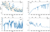 |
Fig. 8. Same as Fig. 7, but for Case C. |
| In the text | |
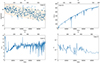 |
Fig. 9. Same as Fig. 7, but for Case D. |
| In the text | |
|
Fig. 10. 3D iso-contours of the tracer (for a tracer value of 0.7), for Case B, at five different times in the interval marked by the black vertical lines in the top right panel of Fig. 7. |
| In the text | |
|
Fig. 11. Longitudinal cut (in the y − z plane) of the distribution of the magnetic field strength at the final times of the simulations. The four panels refer to the four different cases (Case A top-left, Case B top-right, Case C bottom-left, Case D bottom-right). The times are the same as in Fig. 2. |
| In the text | |
Current usage metrics show cumulative count of Article Views (full-text article views including HTML views, PDF and ePub downloads, according to the available data) and Abstracts Views on Vision4Press platform.
Data correspond to usage on the plateform after 2015. The current usage metrics is available 48-96 hours after online publication and is updated daily on week days.
Initial download of the metrics may take a while.