| Issue |
A&A
Volume 685, May 2024
|
|
|---|---|---|
| Article Number | A116 | |
| Number of page(s) | 15 | |
| Section | Extragalactic astronomy | |
| DOI | https://doi.org/10.1051/0004-6361/202348800 | |
| Published online | 15 May 2024 | |
Quasar 3C 47: Extreme Population B jetted source with double-peaked profiles⋆
1
Space Science and Geospatial Institute (SSGI), Entoto Observatory and Research Centre (EORC), Astronomy and Astrophysics Department, PO Box 33679 Addis Ababa, Ethiopia
e-mail: This email address is being protected from spambots. You need JavaScript enabled to view it.
2
Addis Ababa University (AAU), PO Box 1176 Addis Ababa, Ethiopia
3
Jimma University, College of Natural Sciences, Department of Physics, PO Box 378 Jimma, Ethiopia
4
Istituto Nazionale di Astrofisica (INAF), Osservatorio Astronomico di Padova, vicolo dell’ Osservatorio 5, Padova 35122, Italy
5
Instituto de Astrofisica de Andalucía (IAA-CSIC), Glorieta de la Astronomia s/n, Granada 18008, Spain
6
Mbarara University of Science and Technology (MUST), Faculty of Science, Physics Department, PO Box 1410 Mbarara, Uganda
Received:
30
November
2023
Accepted:
20
February
2024
Abstract
Context. An optically thick, geometrically thin accretion disk (AD) around a supermassive black hole might contribute to broad-line emission in type 1 active galactic nuclei (AGN). However, the emission line profiles are most often not immediately consistent with the profiles expected from a rotating disk. The extent to which an AD in AGN contributes to the broad Balmer lines and high-ionization UV lines in radio-loud (RL) AGN needs to be investigated.
Aims. This work aims to determine whether the AD can account for the double-peaked profiles observed in the Balmer lines (Hβ, Hα), near-UV (MgIIλ2800), and high-ionization UV lines (C IVλ1549, CIII]λ1909) of the extremely jetted quasar 3C 47.
Methods. The low ionization lines (LILs) (Hβ, Hα, and Mg IIλ2800) were analyzed using a relativistic Keplerian AD model. Fits were carried out following Bayesian and multicomponent nonlinear approaches. The profiles of prototypical high ionization lines (HILs) were also modeled by the contribution of the AD, along with fairly symmetric additional components.
Results. The LIL profiles of 3C 47 agree very well with a relativistic Keplerian AD model. The disk emission is constrained between ≈102 and ≈103 gravitational radii, with a viewing angle of ≈ 30 degrees.
Conclusions. The study provides convincing direct observational evidence for the presence of an AD and explains that the HIL profiles are due to disk and failed-wind contributions. The agreement between the observed profiles of the LILs and the model is remarkable. The main alternative, a double broad-line region associated with a binary black hole, is found to be less favored than the disk model for the quasar 3C 47.
Key words: quasars: emission lines / quasars: general / quasars: supermassive black holes / quasars: individual: 3C 47
Based on observations collected at the Centro Astronómico Hispano en Andalucía (CAHA) at Calar Alto, operated jointly by the Junta de Andalucía and Consejo Superior de Investigaciones Científicas (IAA-CSIC).
Visiting researcher at the IAA-CSIC, Spain as a PhD fellow.
© The Authors 2024
 Open Access article, published by EDP Sciences, under the terms of the Creative Commons Attribution License (https://creativecommons.org/licenses/by/4.0), which permits unrestricted use, distribution, and reproduction in any medium, provided the original work is properly cited.
This article is published in open access under the Subscribe to Open model. This email address is being protected from spambots. You need JavaScript enabled to view it. to support open access publication.
1. Introduction
In the current working picture of active galactic nuclei (AGN), the underlying power source is thought to be a supermassive black hole (SMBH). An accretion disk (hereafter AD) around the central SMBH is expected in all the AGN. ADs provide an efficient mechanism for dissipating the angular momentum of the accreting matter via viscous stresses (e.g., Shakura & Sunyaev 1973; Dai et al. 2021; Lasota 2023). In addition, they are regarded as an essential ingredient for the production of relativistic jets, which are observed in a considerable fraction of AGN (e.g., Blandford 1990; Shende et al. 2019; Blandford et al. 2019; Chakraborty & Bhattacharjee 2021; Mizuno 2022). High-density material in an AD may be required for the production of the low-ionization lines (LILs) (Rokaki 1997; Zhang et al. 2019b; Hung et al. 2020). Emission from the surface of a photoionized relativistic Keplerian AD produces profiles of double-peaked lines with two distinctive features: (1) a stronger blueshifted peak due to Doppler boosting, and (2) a redward shift that increases toward the line base and is associated with gravitational redshift and a Doppler transverse effect (Chen & Halpern 1989, hereafter CH89). In this respect, the most commonly proposed solution for double-peaked emission from the AD is the assumption of an elevated structure around the inner disk that would illuminate the outer disk and drive the line emission (Strateva et al. 2003; Eracleous & Halpern 2003; Ricci & Steiner 2019).
Even though most AGN spectra are single peaked, there are pieces of evidence of a double-peaked structure that can be acquired from observations of very broad double-peaked emission lines and identification of asymmetries and substructure in the line profiles (e.g., Popović et al. 2002; Kollatschny 2003; Shapovalova et al. 2004). Miley & Miller (1979) found that powerful radio galaxies and radio-loud (RL) quasars with extended radio morphology have the broadest and most complex Balmer line profiles and are preferred hosts of double-peaked emitters. AGN with double-peaked emission lines are an interesting class of objects, even though only a small fraction has been found (e.g., Eracleous & Halpern 1994, 2003; Strateva et al. 2003; Eracleous et al. 2009; Fu et al. 2023). According to Wang et al. (2005), these double-peaked lines are among the broadest optical emission lines, with a full width at half maximum (FWHM) that in some cases exceeds 15 000 km s−1. Following the classification scheme of Sulentic et al. (2002), they are more frequently found in extreme Population B, and, more precisely, in spectral type (ST) B1++. This ST is populated by a tiny minority of quasars in optically selected samples (Marziani et al. 2013b) and is consistently associated with an FWHM Hβ in the range of 12 000–16 000 km s−1 and low or undetectable singly ionized (FeII) emission. They are evolved sources with spectacular extended narrow-line regions (NLRs) and a high prevalence of powerful radio jets (Zamfir et al. 2008; Ganci et al. 2019). In physical terms, sources belonging to this ST are seen at a relatively high inclination and/or have a high SMBH mass (MBH) and very low Eddington ratio (Lbol/LEdd ≈0.01) (e.g., Panda et al. 2019b).
A variety of mechanisms have been proposed to explain the origin of double-peaked emission line profiles and their unique kinematic signature, beyond relativistic motions in an AD (e.g., CH89; Chen & Halpern 1990), such as two separate broad-line regions (BLRs) as a signature of binary black holes (Gaskell 1983), a biconical outflow (Zheng et al. 1990), or a highly anisotropic distribution of emission line gas (Wanders et al. 1995; Goad & Wanders 1996). A careful consideration of the basic physical arguments and recent observational results tends to confirm that the most likely origin of double-peaked emission lines is the AD, and on the other hand, these double-peaked profiles provide dynamical evidence for the structure of the AD (e.g., Chen et al. 1997; Eracleous 1998; Ho et al. 2000; Strateva et al. 2003; Eracleous & Halpern 2003; Barrows et al. 2011; Zhang 2011; Liu et al. 2017; Ricci & Steiner 2019; Zhang et al. 2019a). Several additional observational tests combined with physical considerations also favored the AD origin over other possibilities (e.g., Eracleous & Halpern 1994, 2003; Eracleous 1999; Strateva et al. 2003; Eracleous et al. 2009; Zhang 2013; Wada et al. 2021; Storchi-Bergmann et al. 2017).
Nonetheless, open questions concerning the disk emission in this class of rare AGN remain. UV spectroscopy of double-peaked emitters with the Hubble Space Telescope (HST) did not provide unambiguous evidence for an AD origin (e.g., Halpern et al. 1996; Eracleous 1998; Eracleous et al. 2004; Zhang 2011), and high-ionization lines (HILs; e.g., Lyα and C IVλ1549) frequently lack double-peaked profiles (e.g., Halpern et al. 1996; Murray & Chiang 1997; Eracleous et al. 2004, 2009).
To evaluate the extent to which AD is a source of the broad Balmer lines and UV HILs in RL AGN, we focused on a strong RL quasar, 3C 47 (e.g., Hocuk & Barthel 2010). Previous studies of 3C 47 indicated that it exhibits peculiar broad emission line profiles with multiple components, making it a member of the AGN class of double-peaked emitters (Eracleous & Halpern 2003). This work presents new simultaneous optical and near-UV spectra of the relativistically jetted double-peaked quasar, 3C 47 at redshift 0.4248 from long-slit spectroscopic observations. These new observations of 3C 47 yielded a spectrum with a high signal-to-noise ratio (S/N), high resolution, and broad and strong blue and red peaks that are typical indicators of double-peaked emitters in the Balmer lines (Hβ and Hα) as well as in the near-UV Mg IIλ2800 (hereafter MgII) line. In addition, we also present and interpret the semi-forbidden lines of the λ1900 Å blend, dominated by CIII]λ1909, and the HIL CIVλ1549 from the HST Faint Object Spectrograph (HST-FOS) archive.
The paper is organized as follows: The data used in this work are described in Sect. 2. Spectral nonlinear multicomponent and model fittings as well as a full broad profile analysis are described in Sect. 3. The AD model fit, following the approximation by CH89, was carried out by using Bayesian methods for each of the three spectral regions, MgII, Hβ and Hα, as described in Sect. 3. The results of using a model that for the first time in this object attributes the emission of the double-peaked lines to the surface of a photoionized relativistic Keplerian AD plus the results of the broad profile parameters are described in Sects. 3 and 4. We discuss the resulting accretion parameters, the interpretation of the CIVλ1549 and CIII]λ1909 emission lines, the explanation of the CIVλ1549 profile as due to the contribution of the AD and a failed wind, and the available alternative models in Sect. 5. Finally, our conclusions are given in Sect. 6. Throughout this paper, we adopt a flat ΛCDM cosmology with ΩΛ = 0.7, Ω0 = 0.3, and H0 = 70 km s−1Mpc−1.
2. Data
2.1. Near-UV and optical observations
New long-slit near-UV and optical spectroscopic observations were obtained on the night of 22 October 2012 with the TWIN spectrograph of the 3.5 m telescope at the Calar Alto Observatory (CAHA, Almería, Spain)1. In the sample of 12 extremely jetted RL quasars in the observations of Mengistue et al. (2023, hereafter STM23), 3C 47 was found to possess a double-peaked broad-line profile and was therefore singled out for the more detailed analysis presented in this paper. The observations were obtained with a slit width of 1.2 arcsec. The total exposure time was split into three exposures (of 1200s each) to eliminate cosmic rays by combining different exposures. The mean air mass was found to be 1.09. We obtained high-quality spectra with an S/N of ≈60 in the continuum near Hβ and Hα lines. The observational setup and data reduction of 3C 47 are the same as for the other 11 sources described in STM23. The spectra of 3C 47 reveal three spectacular emission lines corresponding to Hβ and Hα in the red and Mg II in the blue arms of the spectrograph.
We determined the median spectroscopic redshift of 3C 47 by the method detailed in STM23 (Sect. 2.2), in which we measured the observed vacuum wavelength of individual narrow emission lines (e.g., [OII]λ3727, Hγ, Hβ, and [OIII]λλ4959,5007) available in the spectra and found it to be z ≈ 0.4248 ± 0.0004, in fair agreement with the previously measured value of z ≈ 0.4255 (Véron-Cetty & Véron 2010). The basic observational and physical properties of this source are summarized in Table 1 in Cols. 2–10. The rest-frame spectra that provide a concomitant coverage of MgII, Hβ and Hα regions are shown in Fig. 1. 3C 47 has an apparent Johnson magnitude V ≈ 18.1 and is hence relatively bright. The absolute magnitude (MB) of −23.3 (Véron-Cetty & Véron 2010) makes it a rather low luminosity AGN.
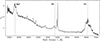 |
Fig. 1. New rest-frame spectrum of 3C 47 that covers MgII, Hβ and Hα. The abscissa is the wavelength in Å and the ordinate corresponds to specific flux in units of 10−15 ergs s−1cm−2 Å−1. The dot-dashed vertical lines trace the rest-frame vacuum wavelength. |
Summary of the general optical and radio properties.
2.2. Archival data
2.2.1. Radio data
3C 47 is a classical powerful Fanaroff-Riley II radio source (Fanaroff & Riley 1974) that is known for a spectacular double-lobed structure with a strong core (Burns et al. 1984). Some basic radio properties, including the radio flux density obtained at 1.4 GHz (21 cm) from the National Radio Astronomy Observatory (NRAO) Very Large Array (VLA) Sky Survey (NVSS)2 (Condon et al. 1998) and the radio spectral index α from Vollmer et al. (2010), are reported in Table 1 (Cols. 11 and 12, respectively). The value listed for the specific flux is the sum of two sources detected by the NVSS, corresponding to the two major lobes. The radio-loudness parameter, which is the ratio of the rest-frame radio flux density at 1.4 GHz to the rest-frame optical flux density in the g band, RK (e.g., Zamfir et al. 2008; Gürkan et al. 2015) as well as the radio power (Pν) using the relation from Shankar et al. (2008 their Eq. (1), also detailed in STM23, Sect. 2.3) are listed in Cols. 13 and 14. In all the calculations, we used the convention for the spectral index, Sν ∝ ν−α. 3C 47 is one of the extreme RL sources with log RK ≈ 4 and high radio power, log Pν ≈ 34.5 [ergs s−1 Hz−1]. These properties are common among double-peakers. Double-peaked emitters are more likely to belong to RL AGN, and they did not show special radio properties (e.g., Eracleous 1998; Strateva et al. 2003). Further details of the relation between optical and radio properties are provided in Sect. 5.3.
2.2.2. UV data
The UV data were obtained from the HST-FOS3 archive. The resulting rest-frame UV spectra, covering C IVλ1549, HeIIλ1640, and CIII]λ1909 regions are shown in Fig. 2. The detailed disk profile analysis for this band is presented in Sect. 3.1 and discussed in Sect. 5.4.
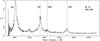 |
Fig. 2. HST/FOS rest-frame spectrum of 3C 47 that covers Lyα, CIVλ1549, HeIIλ1640, and CIII]λ1909. The dot-dashed vertical lines trace the rest-frame vacuum wavelength. The ordinate corresponds to specific flux in units of 10−15ergs s−1 cm−2 Å−1. |
2.2.3. Optical data
To examine an alternative scenario (detailed in Sect. 5.5) as an explanation of the observed double-peaked profile, two additional previously observed optical spectra were retrieved, namely, an ESO spectrum obtained at the 1.52 m telescope on October 14, 1996 (Marziani et al. 2003), and a spectrum obtained at the Copernico telescope equipped with AFOSC on November 27, 2006, covering Hβ and MgII (Decarli et al. 2008).
3. Spectral analysis
We implemented two types of fittings for each of the spectral regions: (i) a model fitting by using a relativistic Keplerian AD model, and (ii) an empirical multicomponent nonlinear fitting of the continuum and the emission features by using IRAF task specfit (Kriss 1994).
3.1. Accretion disk model
We applied the model of CH89, in which AD emission surrounding a single SMBH is assumed to be the origin of double-peaked broad emission lines observed in our spectra. The model assumes that a uniform axisymmetric disk model produces double-peaked line profiles, with the blue peak stronger than the red peak due to Doppler boosting. In the CH89 model, the emission is driven by illumination of the outer part of the disk from an elevated or vertically extended structure. This structure could be an ion-supported torus that photoionizes the geometrically thin outer disk to produce the observed disk line profiles. This ion torus emits harder than that of the standard geometrically thin, optically thick AD, and this property may overcome difficulties associated with the energy budget of the AD. Other illumination geometries may also be possible (e.g., Dumont & Collin-Souffrin 1990).
We used the integral expression for the line profile of an optically thick AD (Eq. (7) of CH89) to fit the double-peaked profiles observed in our spectra. The model includes five crucial and freely varying parameters: the two line-emitting portions at different radii, the inclination angle, the broadening parameter, and the line emissivity index. The line-emitting portion of the disk is assumed to be an annulus with inner and outer disk radii ξ1 and ξ2 respectively, in units of gravitational radius, rg = GMBH/c2.
This model also assumes that the double-peaked emission line originates from the surface, whose axis is inclined by an angle θ relative to the line of sight, between the two radii. Electron scattering or turbulent motion is assumed to be the cause of the line broadening and is represented by a Gaussian profile of the velocity dispersion σ expressed in km s−1 in the rest-frame of the emitter. An axisymmetric emissivity that varies continuously is represented as a function of the radius of the disk (Q) and a dimensionless power-law index q as Q = ξ−q.
3.2. Bayesian fit to the accretion disk model
The fit of the observed broad-line profiles of 3C 47 to the AD model was carried out by using the Bayesian method independently for each spectral regions: MgII, Hβ, and Hα.
The input double-peaked broad emission lines were obtained after removing the other components: that is, mainly the power law of the continuum, the FeII template, and the narrow components (NCs), as explained in Sect. 3.3.1.
A first estimate of the parameters {q, σ/ν, ξ1, ξ2, θ} was obtained by evaluating the χ2 of the fit of the broad profiles to the function defined by Eq. (7) of CH89 for several thousand combinations. This was done to obtain a physically possible range of values that was compatible with the observed double-peaked profiles, as well as initial estimates for each parameter. After inspecting the distribution of χ2 for the MgII, Hβ and Hα we can ensure that for values outside the range of the parameters given in Table 2, χ2 grows monotonically outward. A nonlinear least-squares (as well as a maximum likelihood) fit was obtained by using the midpoints of the ranges as initial values, resulting in parameter solutions that are contained well inside the ranges in all the lines.
Model parameter input list.
In addition, we applied a Monte Carlo Markov Chain (MCMC) approach, where we obtained model approximations using the emcee: The MCMC hammer package (Foreman-Mackey et al. 2013), which is based on slight modifications to the Metropolis-Hastings method. For the Bayesian inference, we used two different prior functions (p(η)): (1) a uniform prior for each AD model parameter with the range of values listed in Table 2,
and (2) Gaussian distribution priors with central values corresponding to the midpoints described previously, and σ guaranteeing the full range of parameters to be sampled
with ηc and ση describing the center and spread of each probability p(η) prior. In a way that the total prior is the product of each parameter prior distribution p(η),
In our case, the two sets of priors provide the same results with negligible differences between them, and they are well within the posterior distributions. Figure 3 shows the corner plot (left panel) and 250 randomly selected posterior solutions (right) for the AD model (green lines) over the broad double-peaked profile (red) of MgII. The corner plot shows the covariances and posteriors of the five parameters for the fit, in which we display at the top of each posterior distribution the median value of each parameter and the errors measured as percentiles at the 0.135% and 99.865% levels (which correspond to 3σ errors in a normal distribution). In Fig. 4 we show the corner plots for Hβ (left panel) and Hα (right). Table 3 contains the final measurements of the five model parameters for MgII (Col. 2), Hβ (Col. 3) and Hα (Col. 4) and the corresponding uncertainties.
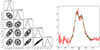 |
Fig. 3. Left: Corner plot showing the posterior distributions of the five AD parameters for MgII as histograms, along with covariance maps between the parameters. Right: 250 randomly selected posterior solutions from the Bayesian fit (green) superimposed onto the observed broad profile (red) of MgII. |
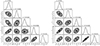 |
Fig. 4. Corner plots for Hβ (left panel) and Hα (right). |
Summary of the output parameters from the Bayesian inference model fittings.
3.3. Empirical fittings
3.3.1. MgII. Hβ and Hα
A nonlinear multicomponent fitting procedure by using specfit was implemented to obtain a global fitting in each spectral range. We followed the same method as described in STM23. The specfit fittings were performed twice. First, to represent the observed broad profile of each double-peaked line of interest (i.e., for Hβ, MgII and Hα), we assumed two Gaussian broad components (BC) of the same FWHM (corresponding to the blue and red components of the double-peaked profile) and a very broad component (VBC), which allowed us to isolate the broad profile in each spectral region after removing other components and to obtain the AD model parameters from the Bayesian fit, as explained in Sect. 3.2. In the second fitting, the resulted AD model was introduced to represent the broad profile instead of the initial 2BC + VBC.
In these fittings, we also included a power-law local continuum (Shields 1978), an FeII template to model the FeIIopt and FeIIUV using the templates from Marziani et al. (2009) and Bruhweiler & Verner (2008), respectively, and an additional UV Balmer continuum, found to be important at λ < 3646 Å in the region of MgII (Kovačević et al. 2014; Kovačević-Dojčinović et al. 2017). In addition, to represent the nondisk emission components, we included Gaussian profiles to fit the narrow and semi-broad components (NC + SBC) from the NLR. All the narrow lines were assumed to have roughly the same width and shift values.
In the Hβ region, the overall fitting was made in the wavelength range from 4400 Å – 5300 Å. In addition to the AD broad component, this includes the [OIII]λλ4959,5007 and HeIIλ4686 lines in addition to the Hβ NC + SBC. The Hα region final fit was made from 6100 Å – 6900 Å. To obtain the best empirical fitting of the Hα + [NII] blend, we included, together with the AD model output representing the broad profile, Gaussians NC + SBC for Hα, [OI]λλ6302,6365 and for the doublets of [NII]λλ6549,6585 and [SII]λλ6718,6732. A power law that defines the continuum and the FeII template was also added. The near-UV MgII region was fit in the wide wavelength range from 2600 Å – 3800 Å, which includes the doublet NCs of Mg II, and OIIIλ3133 Å, [OII]λ3727 Å, and the two HILs of [NeV] at λλ3346,3426 Å.
The resulting specfit fits, including the AD model for the observed broad profiles as well as the nondisk emission components with a minimum χ2 in the regions of Hβ, Hα, and MgII, are shown in Figs. 5–7, respectively, on a rest-frame wavelength scale.
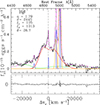 |
Fig. 5. Multicomponent empirical specfit analysis, including the AD model fitting result in the Hβ region after subtracting the continuum from the best fit. The upper abscissa is the rest-frame wavelength in Å and the lower abscissa is in radial velocity units. The vertical scale corresponds to the specific flux in units of 10−15 ergs s−1 cm−2 Å−1. The emission line components used in the fit are FeII (green), the broad AD model representing the fit for the broad double-peaked profile (red line), SBC (orange), and NC (blue). The black continuous line corresponds to the rest-frame spectrum. The dashed magenta line shows the final fitting from specfit. The dot-dashed vertical lines trace the rest-frame wavelength of Hβ. The lower panel shows the residual of the empirical fit. |
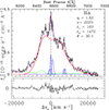 |
Fig. 6. Multicomponent empirical analysis and AD model fitting results in the Hα region. The description is as in Fig. 5. |
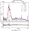 |
Fig. 7. Multicomponent analysis and AD model fitting results in the MgII region. The description is as in Fig. 5. |
3.3.2. Civλ1549 and Ciii]λ1909
Theoretical predictions and studies of double-peaked profile sources indicate that the disk predominantly emits LILs (e.g., Balmer lines, MgII and FeII). High-ionization species such as CIVλ1549 may not be produced and may lack double-peaked profiles even when the LILs do show them (e.g., Collin-Souffrin & Dumont 1990; Eracleous & Halpern 1994; Eracleous 1998; Tang & Grindlay 2009).
In addition to the LILs, we also fit the available HIL: C IVλ1549, HeIIλ1640, and CIII]λ1909. The CIVλ1549 line region was fit in the spectral window 1420 Å-1705 Å and modeled by the contribution of the AD, along with prominent additional components including a symmetric Gaussian and two blueshifted CIVλ1549 components associated with a failed-wind scenario, NIVλ1483, 5 absorption lines eating away the NLR contribution to C IVλ1549, a blueshifted SBC for HeIIλ1640, and OIIIλ1663. For the CIII]λ1909 line profile, we considered the spectral window 1850 Å –1920 Å, which includes two AlIIIλλ1857,1862, SiIII]λ1892, CIII]λ1909 and two absorption lines. We also assumed an NC for CIII]λ1909. The resulting fits for the CIVλ1549 and CIII]λ1909 regions are shown in Figs. 8 and 9, respectively. A discussion of the assumptions and the resulting fitting is presented in Sect. 5.4.
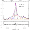 |
Fig. 8. Multicomponent empirical analysis and AD model fitting results for CIVλ1549 and HeIIλ1640. The black line corresponds to the rest-frame spectrum, and the emission line components used in the empirical fit are the blueshifted components (blue) and BC (black). The red line represents the model fitting result for CIV and HeIIλ1640 by using the AD model fitting parameters of Hβ. The dashed magenta line shows the final model fitting from specfit. The lower panel shows the residuals. |
4. Results
4.1. AD model parameters
The resulting quantitative measurements of the AD model, that is, {q, σ, ξ1, ξ2, θ}, determined by following the approach described in Sect. 3.1 for the Mg II, Hβ, and Hα regions are reported in Table 3. The line-emitting portion of the disk was found to be an annulus within ξ1 ≈ 100rg and ξ2 ≈ 1000rg, with the highest values ξ1 ≈ 131rg and ξ2 ≈ 1632rg estimated for MgII. The ratio of the outer to inner radius ξ2/ξ1 is ≈10, 12, and 14 for Hβ, MgII and Hα, respectively. A higher value of the ξ2/ξ1 ratio will bring the blue and red peaks close together and will form a single peak.
We found a range of inclination angles relative to the line of sight between the two radii. The lowest inclination of θ≈ 26.7° was found for the Hβ line, and the highest inclination of θ ≈ 32.6° was found for Mg II. The average value of θ is ≈29.8 ± 3.0 or ≈30 °.
The emissivity index ranges between 1.62 (Hα) – 1.79 (Hβ). The factor that represents the turbulent motion and is assumed to be the cause of local line broadening was represented by σ/ν0. We found the highest value of σ/ν0 = 8.156 × 10⁻³ for the Hβ and the lowest for Mg II, of σ/ν0 = 5.827 × 10⁻³. This value of σ/ν0 corresponds to a velocity dispersion σ that is higher in Hβ, with a value of 2445 km s−1 and lower in MgII, with a value of 1747 km s−1. These values are comparable to the values obtained from the AD model fitting of other double-peaked AGN (e.g., Eracleous 1998; Strateva et al. 2003).
4.2. Empirical fitting results
We employed a comprehensive parameterization of the broad profiles involving the total flux, FWHM, and centroids at different fractional line intensities (c(i/4) for i = 1, 2, and 3) and 9/10, c(9/10) (a proxy to the line peak), as well as asymmetry (AI) and kurtosis (KI) indices (Zamfir et al. 2010). The 3C 47 parameters are reported in Table 4 for MgII, Hβ and Hα. The broad-line fluxes (Col. 2) and the specific fluxes of the power-law continuum (Col. 10) along with the FWHM (Col. 3) were used to compute the accretion parameters ( see Sect. 5.1).
Measurements of the full broad profile and the NC + SBC of the three analyzed lines.
3C 47 shows a very large line width with an FWHM of ≳15 000 km s−1. The Hβ disk line profile is one of the broadest, with an FWHM of 16 600 km s−1. The centroid velocity measurements at different fractional intensities show a predominance of shifts to the red. They are more pronounced toward the line base, with c(1/4) ≈ 1650±460 km s−1. Within the uncertainty level, the redward asymmetry appears to be consistent across all three lines, with Hα showing a slightly more symmetric distribution than Hβ and MgII.
The flux of the FeII emission integrated for MgII, Hβ, and Hα regions are reported in Col. 11 of Table 4. With an intensity ratio of approximately 0.14 for RFeII, opt = I(Fe IIλ4570)/I(Hβ), 3C 47 falls within the realm of extreme Population B on the optical plane of the quasar main sequence (MS), defined by the relation between Hβ FWHM and RFeII, opt (Sulentic et al. 2002). More precisely, its Hβ FWHM of ≈16 000 km s−1 places it in the B1++ ST according to the classification scheme of Sulentic et al. (2002). It is noteworthy that this ST comprises a minimum fraction (lower than 1%) of optically selected quasars with weak or undetectable FeII emission (Marziani et al. 2013b). Ganci et al. (2019) revealed a higher prevalence of irregular or multiple peaked profiles in this ST and suggested a higher prevalence for binary SMBH candidates (see Sect. 5.5).
Columns 1–9 of Table 5 report the full broad profile parameters for the far-UV (FUV) lines, mirroring the organization of Table 4 along with the specific flux (Col. 10). A key result is that the FWHM CIVλ1549 ≪ FWHM Hβ, which is discussed in more detail in Sect. 5.4. The highly blueshifted semi-broad features (blue lines in Figs. 8 and 9) visible for both CIVλ1549 and CIII]λ1909 are probably part of a continuum of outflowing gas from the outer BLR to the inner NLR. Their fluxes are much lower than those of the other components. This may indicate that outflows may have little effect over the integrated line profiles (see Sect. 5.4 for more detail).
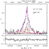 |
Fig. 9. Multicomponent nonlinear empirical specfit and AD model fits for CIII]λ1909 blend following the same approach as employed for CIVλ1549. The axes and the components are the same as in Fig. 8, except for the red line, which represents the AD model fitting result for CIII]λ1909, SiIII]λ1892, and the sum of the two AlIIIλ1857 components by using the parameters appropriate for the MgII. The resulting Si III]λ1892 is barely visible. The black lines trace the BC components of CIII]λ1909 and Si III]λ1892. The dot-dashed vertical line identifies the rest-frame wavelength of CIII]λ1909. |
Measurements of the full broad profile and the NC + SBC of the FUV lines.
In addition to the parameters of the broad profiles, we report the flux, the peak shift, and the FWHM for NCs and SBCs of identified emission lines from the specfit analysis (Tables 4 and 5). Individual NCs are near the rest-frame, with a broad FWHM of 840 km s−1 for Hα and a slightly lower value for Hβ and Mg IIλ2800. The CIVλ1549 NC is absorbed by narrow lines close to the rest-frame.
Finally, Table 6 reports the total intensity, peak shift, and FWHM for additional narrow and semi-broad emission lines identified in the four spectral ranges (MgIIλ2800, Hβ, Hα, and CIVλ1549).
Narrow lines and narrow-line components.
5. Discussion
5.1. Accretion parameters
Black hole masses (MBH) were computed from the virial equation applied in the form of a scaling law (SL), where MBH was assumed to be proportional to the square of the line width (Vestergaard & Peterson 2006), and the BLR radius was estimated from its correlation with the continuum or luminosity of different emission lines (Shen & Liu 2012; Bentz et al. 2013). Alternatively, the line width can be increased to a power different from the second (Shen & Liu 2012). This approach has been extensively applied in previous studies, including large samples of quasars from the Sloan Digital Sky Survey (SDSS) (e.g., Kozłowski 2017 and references therein).
An important input parameter does not explicitly appear in the SLs: the viewing angle (θ) between the line-of-sight and the axis of symmetry of the AGN (i.e., the AD axis or the radio axis). Double-peaked sources such as 3C 47 presumably have almost all of their low-ionization emission lines modeled by a geometrically thin, optically thick disk, and it is therefore easy to associate a well-defined θ with the line FWHM (for an alternative approach, see e.g., Bian et al. 2007).
When the inclination angle derived from the disk profile analysis is taken into account, the virial relation can be written as
 (1)
(1)
where δvK is the Keplerian velocity of the line emitting gas at the radius of the BLR (RBLR). The virial factor f(θ) connects δvK to the observed FWHM and can be written as (e.g., Decarli et al. 2008; Mejía-Restrepo et al. 2018; Negrete et al. 2018):
![Mathematical equation: $$ \begin{aligned} f(\theta )=\frac{1}{4[k^2 + \sin ^{2}\theta ]} , k=\frac{\sigma { v}_{\rm iso}}{\sigma { v}_{\rm K}}\approx 0.3 \end{aligned} $$](/articles/aa/full_html/2024/05/aa48800-23/aa48800-23-eq28.gif) (2)
(2)
f ≈ 0.735 when θ ≈ 30.
Table 7 reports the line or continuum identifications and the corresponding luminosity values (Cols. 1 and 2, respectively), the BLR radius estimated from its correlation with luminosity (Col. 3), the method used (either using Eq. (1) above, or an SL that directly links the mass to the luminosity and line width, Col. 4), the estimated MBH (Col. 5), and the Eddington ratio (Lbol/LEdd) (Col. 6) for several different SL (in Col. 4, with reference in Col. 7) using Hβ, MgII and Hα as virial broadening estimators.
Accretion parameters.
The Lbol/LEdd was computed from the 3C 47 spectral energy distribution (SED) as available in the NASA/IPAC Extragalactic Database (NED). The mid-IR (MIR) and far-IR (FIR) emissions were cut to avoid the inclusion of reprocessed radiation and unresolved emissions not associated with the AGN. The resulting bolometric correction factors are 25.59 from λfλ 5100 Å and 16.39 from λfλ3000 Å, which is considerably higher than in the case of optically selected RQ quasars, ≈10–15 from λfλ 5100 Å (Richards et al. 2006; Punsly et al. 2020). For 3C 47, the bolometric correction includes the accretion luminosity (i.e., from the AD and associated coronæ), as well as the emission associated with the relativistic jet. A flat X-ray SED, expected to be due to synchrotron self-Compton (SSC; Maraschi et al. 1992) emission, produces a luminosity of log LX ≈ 46.28 [erg s−1], which contributes up to ≈ 40 % of the bolometric luminosity log L ≈ 46.64 [ergs s−1]. For comparison, a Population A AGN SED (corresponding to the Mathews & Ferland (1987) template, as implemented by the command table AGN in CLOUDY) with the same optical flux as 3C 47 would yield log LX≈ 45.24 versus log L≈ 46.32 [ergs s−1] (e.g., Lusso et al. 2012). The Lbol/LEdd estimated from the average of the three MBH determinations from Eq. (1) is Lbol/LEdd ≈ 0.040 ± 0.012, including the accretion and nonthermal emission. The SSC emission may be beamed; however, beaming effects on the optical/UV synchrotron continuum are probably minor, as confirmed by the MBH estimates based on continuum measurements, which are consistent but slightly lower than those based on emission lines for which no beaming effect is expected.
5.2. AD as the origin of the double-peaked profile
Two pieces of evidence support an illuminated AD as the main source of LILs (see Sects. 3.2 and 4, and Table 3):
-
The two peaks are well separated, implying a disk of modest extension with ξ2 ≈103rg.
-
The overall profile is asymmetric due to relativistic beaming (Doppler-boosted peak) and gravitational redshift of the entire line (redshifted line base).
The most remarkable finding is that the ξ1 should be as low as ≈100 rg, implying a large shift because of gravitational and transverse redshift, cδzgrav ≈ 3/2 ξ1 ≈ 4500 km s−1. It is also remarkable that the predicted shape provides a good fit for the line red wings. 3C 47 is not an exception in this respect because blazars also show red asymmetric disk profiles characterized by large shifts at the line base, consistent with emission from the innermost disk (see e.g., Punsly et al. 2020; Marziani 2023). In the case of blazars, the orientation angle is θ ≲ 5°, however, and consequently, the profiles appear to be single peaked (Decarli et al. 2011; Marziani 2023).
The decreasing line width in the order Hβ, Hα, and MgII is associated with a difference in the emissivity-weighted radius of the three lines. The MgII is emitted by a region of the disk that is weighted toward larger radii than Hβ and Hα (see Table 3, Cols. 2, 3, and 4). This effect is seen in Population B sources where emission is dominated by a virial velocity field (Marziani et al. 2013a, STM23), for which the line width is inversely proportional to the square root of the distance from the central continuum source, that is, an FWHM  .
.
In summary, the three LILs show profiles that are consistent with a relativistic flat AD, and their main features can be explained by the physical processes expected to occur for ionizing continuum radiation reprocessed by the disk. This, however, is not the case for HILs ( see Sect. 5.4 for more details).
5.3. Consistency between radio and optical properties
Assuming that the relativistic jet is coaxial with the disk, that is, the jet axis and the disk plane are perpendicular, an interesting issue is whether the orientation of the jet is consistent with the inclination of the AD. The radio morphology is double lobed, with jet, but no counterjet is easily visible at 4.9 GHz (Fernini et al. 1991). The jet-counterjet asymmetry implies the presence of a highly relativistic jet, and along with the double-lobe morphology, a significant misalignment between the jet axis and the plane of the sky as well as with the line of sight. Superluminal motion has been detected by VLBI observations of 3C 47, with an apparent superluminal speed of  (Vermeulen et al. 1993). A high superluminal speed like this is incompatible with an angle as large as 30°, as the upper limit to θjet is ≈20° with Lorentz factor γ ≈ 10. However, considering that the uncertainties in the superluminal speed translate into
  , the difference between θjet and θdisk ≈ 30 ± 3 is significant at only slightly more than the ≈1σ confidence level. It is also important to remark that the 3C 47βapp might be overestimated, as this source is an outlier in the correlation between βapp and deboosted core-to-lobe ratio, in the sense that the 3C 47βapp is much higher than expected for its core-to-lobe ratio (Vermeulen et al. 1993).
The ratio of the jet-to-counterjet flux offers an independent test of consistency for the angle θjet. The counterjet is not visible, but an upper limit to the flux is ≈4.2 mJy (Bridle et al. 1994), yielding a lower limit to the jet-to-counterjet ratio ≈5.5. This in turn implies that γ ≳ 2.5 for θ ≈ 29.
Therefore, we conclude that the radio-derived angle between the line of sight and the jet and between the line of sight and the disk axis, θjet and θdisk, are not significantly discordant, leaving open the possibility of slight bending of the parsec-sized jet over scales ≈104rg (Yuan et al. 2018, and Sect. 5.5).
5.4. A failed-wind signature
The most striking result is the obvious difference between the profiles of the LILs and HILs. Unlike in the case of Population A sources, where the CIVλ1549 profile is usually broader and blueshifted in comparison to the Balmer lines, we can explain the CIVλ1549 profile for several Population B RL sources as caused by the disk profile in addition to the emission from a strong, narrower feature (FWHM ≈4000 km s−1) that peaks at the rest-frame and has a slightly asymmetric profile. The origin of this feature is discussed below.
As mentioned above, the interpretation of the so-called double-peakers (CH89; Eracleous & Halpern 1994; Strateva et al. 2003) is that the LILs are produced exclusively through reprocessing of the gas of the AD. The contribution from the disk is expected in the general AGN population, but is thought to be masked by emission due to the gas surrounding the disk itself (Popović et al. 2004; Bon et al. 2009). Therefore, double-peakers in this interpretation are low radiators and sources with little gas left and with a disk truncated at ξ2 ≲ 103rg (Marziani et al. 2021). In addition, jetted sources are X-ray bright and may induce a high-ionization degree (an over-ionization of the gas; Murray et al. 1995; Murray & Chiang 1997). In a line-driven wind scenario, the ionic species yielding the main resonant transitions that absorb the continuum momentum are replaced by higher ionization species, and the gas can no longer be efficiently accelerated (e.g., Murray et al. 1995; Proga & Kallman 2004; Higginbottom et al. 2024, and references therein). This scenario may apply to 3C 47. We considered the disk radii that correspond to linear distances of ≈1017(rg/100) cm, assuming MBH ≈ 6.5 × 10⁹ M⊙, and an array of photoionization simulations assuming as input (1) the SED of 3C 47 as derived from the NED data; (2) radii in the range log ξ2 ≈ 17 − 19 [cm]; (3) hydrogen density between log n ≈ 10 [cm−3] and log n ≈ 12 [cm−3], with steps of 0.5 dex; (4) a metallicity Z at 0.1 and 1 Z⊙; and (5) 0 turbulence broadening.
The first basic result is that the kinetic temperature is too high for a meaningful photoionization solution for moderate densities log nH ≈ 9 and ≈10 at ξ ≲ 1000rg, and ≲500 rg, respectively. This implies that the bulk of the HILs might come from a region beyond the outer edge of the AD. The SED of 3C 47 induces an overionization of the emitting gas, where a photoionization solution is possible. Figure 10 shows that the C3+ ionic stage is only marginally dominant in a narrower range of depth with respect to a cloud illuminated by a typical AGN continuum for the same optical luminosity and all other conditions kept fixed. As a consequence, the force multiplier remains systematically lower for 3C 47 (right panel of Fig. 10), implying that a radiation-driven outflow is disfavored in this case. Another important factor hampering a radiation-driven outflow is the very low Lbol/LEdd: radiation forces become dominant only at low column density (Netzer & Marziani 2010). Most of the optically thick gas will remain bound to the gravitational field of the black hole and reflect the Keplerian kinematics associated with the rotating disk. The modest blueward asymmetry of the C IVλ1549 profile is consistent with a small fraction of the line emitting gas showing a radial velocity associated with outflow motions.
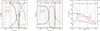 |
Fig. 10. Ionization structure within a gas slab with a column density Nc = 1023 cm−2, log of the hydrogen density 10.0 [cm−3], and distance from the continuum sources log r = 18 [cm] corresponding to ≈1000 rg, where the illuminated surface is at a depth h = 0 (left side), for the continuum of 3C 47 (left panel), and for a typical AGN continuum normalized to the same optical luminosity (middle panel). Rightmost panel: Force multiplier (filled lines) and kinetic temperature (dashed lines) as a function of the geometrical depth of the gas slab for 3C 47 (red) and an AGN continuum (black). |
We can constrain the radial extent of the BLR from the radius r1000 at which the AD temperature is 1000 K to the radius of dust sublimation rdust (Czerny & Hryniewicz 2011). The radius r1000 can be written as
 (3)
(3)
where Ṁ is the accretion rate, σB is the Stefan-Boltzmann constant, and ṁ is the dimensionless accretion rate in Eddington units, that is, ṁ = Ṁ/(L/c2). For the parameters of 3C 47, we obtain that r1000 ≈ 9.3 × 1017 cm ≈940rg. The ratio of rdust and r1000 is (e.g., Czerny & Hryniewicz 2011),
 (4)
(4)
This implies that in the case of 3C 47, the BLR extension is between 1000 rg and ≈12 000rg ≈ 1019 cm. At 5000 rg, the virial velocity is ≈4000 km s−1, in agreement with the expected FWHM considering θ ≈ 30. The FWHM of the symmetric Gaussian CIVλ1549 emission feature is therefore consistent with emission concentrated toward the outer region of the permitted space. This accounts for the separation from the disk that emits lines from within 2000 rg.
The key differences between RL and RQ AGN lie in the configuration of the magnetic field and the SMBH spin, which can significantly impact any radiation-driven wind dynamics (Blandford & Znajek 1977; Blandford & Payne 1982), although the exact roles remain debated. The mildly ionized wind traced by C IVλ1549 still exists in RLs, but is quantitatively affected (Marziani et al. 1996; Richards et al. 2011). The effect of the jet might ultimately be associated with a cocoon of shocked gas that develops where the pressure exerted by later expansion of the jet equals the pressure of the ambient medium. This in turn may displace the launching radius of the wind outward (Sulentic et al. 2015). Therefore, we do not expect a substantial difference between RQ and RL in the occurrence of failed winds, except for the displacement of the launching radius and a lower force multiplier implied by an SED such as that of 3C 47, which would somewhat favor wind failure in RLs.
5.5. Explanations alternative to AD: A binary broad-line region
In an alternative scenario, the observed double-peaked profiles could be attributed to emission from a twin BLR associated with a supermassive binary black hole. Under this assumption, each of the black holes has an associated BLR, and the orbital motion of the binary system produces Doppler shifts in the emission lines that result in the observed double-peaked profiles (e.g., Begelman et al. 1980; Begelman & Meier 1982; Gaskell 1983; Peterson et al. 1987; Chornock et al. 2010). The hypothesis of a binary black hole appears debatable on the basis of radio data. On the one hand, there is no evidence of an obvious S-shaped configuration of the jet. The 3C 47 jet extends over ≈200 kpc and shows the smallest bending measures (≲8 degrees) of several double-lobed sources (Bridle et al. 1994). The position angle of the parsec-scale jet mapped by VLBI (Yuan et al. 2018) is consistent with the jet mapped by the VLA. This evidence favor the stability of the jet orientation over the dynamical timescale of the radio source, ≈6 × 10⁷ yr (Turner et al. 2018). On the other hand, the presence of a secondary SMBH is indicated by three subtle pieces of evidence (Krause et al. 2019): (1) a jet at the edge of the lobe; (2) a ring-like feature that is well visible in the southern lobe (Fernini et al. 1991; Leahy 1996); and (3) the S-symmetry of the hot spots with respect to the jet axis, and an estimate of the geodetic precession timescale (Barker & O’Connell 1975),
 (5)
(5)
where  is the mass ratio (assumed here to be
  ), and r = a, the semimajor axis of the orbit for an eccentricity e = 0, in parsecs. In the case of 3C 47, PG is lower than (for MBH ≈ 6 × 10⁹ M⊙) or comparable to the dynamic age of the radio source, and it is therefore compatible with the features seen in the radio lobes.
To examine whether this interpretation is a possible mechanism for the observed double-peaked profile in the spectra of 3C 47, we recovered two additional spectra obtained in the epoch preceding 2012 (see Sect. 2.2). The spectra were normalized to the sum of the [O III]λ5007 NC + SBC. A previously unreported result is that the broad emission in 1996 was extremely faint and could have escaped detection if the more recent spectra had not been available for comparison: The Hβ broad profile strength in 1996 was about one-third and about half of those measured on the 2006 and 2012 spectra.
The total mass of the binary M = M1 + M2 can be estimated from the observed spectra using the third Kepler law. We used the equations from Eracleous et al. (1997) to estimate M, which corresponds to the period and orbital velocities,
 (6)
(6)
where v1 is the orbital velocity of M1 normalized to 5000 km s−1, and P is the orbital period in units of 100 yr. The v1sin θ corresponds to the radial velocity of the blue peak (vr Blue) and the v2sin θ to the red peak (vr Red). We did not use v2 because the red peak wavelength is very poorly constrained. The projected peak velocities were estimated from the empirical fittings of the lines using two Gaussian profiles as a BC to represent the two peaks. For the Hβ line of the 2012 spectrum (presented in this paper), the corresponding blueshift and redshift velocities were found to be ≈–3200 km s−1 and ≈ +5000 km s−1, respectively, from the peak flux in the observed double-peaked profile fitted as shown in Fig. 11 for Hβ and MgII. For Hα, the blue peak is located around −2800 km s−1 and the red peak is found at +5900 km s−1, yielding  and ≈2.11 for Hβ and Hα respectively. An average over Hβ, MgII and Hα at all available epochs consistently yields
  for the putative binary. The high dispersion reflects the difficulty in carrying out precise measurements of peaks of broad features that are affected by atmospheric absorption as well as strong overlying [O III]λλ4959,5007 emission (red peak of Hβ). The results for the measurements of Hβ and MgII are reported in Table 8. The 1996 spectrum yields very poor constraints on the blueshifted peak, with vr Blue
  km s−1 at 1σ confidence level.
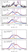 |
Fig. 11. Top: Multicomponent empirical specfit analysis results in the Hβ line region for three epochs after subtracting the power-law and the Balmer recombination continuum (the latter for the MgII spectral range). The abscissa is in radial velocity units. The vertical scale corresponds to the specific flux in units of 10−15 ergs s−1 cm−2 Å−1. The emission line components used in the fit are FeII (green), the blue- and red-peaked profiles (black), the VBC (red), and the full profile (sum of the two BCs and the VBC; thick black), all the NCs (blue), and [OIII]λλ4959,5007 SBC (orange). The continuous black lines correspond to the rest-frame spectrum. The dashed magenta line shows the model fitting from specfit. The dot-dashed vertical lines trace the rest-frame wavelength of Hβ. The dotted lines identify the radial velocity of the blue- and redshifted broad Gaussian components. Bottom: Same for the MgII line after removing the FeII emission for clarity. |
Measured shifts of broad-line profiles and lower limits on MBH.
The only parameter that needs to be determined in Eq. (6) is the period from the displacement of the observed spectra. We focused on the blueshifted peak of Hβ. To estimate the period, we considered the Δv over the time span Δt, and the radial velocity span v2 − v1 (i.e., the separation of the two peaks). In the case of a circular orbit, the period should be P ≈ 2(v2 − v1)/Δv × Δt, and the values are reported for the Hβ and MgII in the cases of the full double-peaked profile and the fitting components. θ is known to be ≈20 − 30 degrees (Sect. 5.3), so that all observed radial velocities are to be divided by sin θ which we assumed here to be ≈30.
The second half of Table 8 provides the estimates of periods and total binary black hole masses from the shift variation in Hβ and MgII over the time lapses between observations. The most constraining limit in Eq. (6) comes from the measurement of the Hβ peak: The Δv ≲ 1100 km s−1 implies a period of P ≳ 200 yr, and MBH ≈5 ⋅ 1010 M⊙, which is above the estimates of Sect. 5.1. The uncertainty of the 1996 measurement is large; the −1σ limit would imply a displacement of just 120 km s−1 with respect to the 2012 measurement, implying P ≈ 2800 yr and MBH ≈4 × 10¹¹ M⊙. In addition, the measurements between 2006 and 2012 show that there is no evidence of strong changes in the radial velocity of the blue peak. Even if there is an apparent systematic increase in the shift for both Hβ and MgIIλ2800, the change in the red peak may not be consistent with an orbital motion around a common center of mass. We can conclude that there is no evidence in favor of a binary BLR given the constraints on the mass of the putative binary black hole and the uncertainties in the data. Further spectroscopic monitoring is needed to fully dismiss this possibility.
However, assuming that a second black hole affects the shape of the line profile in a periodic way, we write the relation between the geodetic precession and orbital period as
 (7)
(7)
The separation of the two black holes is basically unconstrained, but an upper limit on PG is given by the dynamic age of the radio source, ≈6 × 10⁷ yr. With the black hole mass of 3C 47, the age would imply a radius of ≈100 pc. Smaller radii might be possible; since 1 pc ≈3000 rg, it is tempting to speculate that a second black hole within a few parsecs from the primary might cause the truncation of the disk at ≲2000 rg.
5.6. Further alternatives
Another scenario proposed for the explanation is emission from the oppositely directed sides of a bipolar or biconical outflow. In this scenario, the double-peaked lines originate in pairs of oppositely directed cones of outflowing gas that are accelerated by the passage of the relativistic radio jets through the line-emitting region and interaction with the gas immediately around the central engine (e.g., Norman & Miley 1984; Zheng et al. 1990; Sulentic et al. 1995). Evidence of line broadening after a flare-like event has been found (León-Tavares et al. 2013; Chavushyan et al. 2020), and can be interpreted as an unresolved bipolar outflow. These phenomena, however, are transient over timescales of years or shorter. Gas moving at ≈4000 km s−1 for slightly less than 20 years would imply a displacement of ≈0.1 pc. Maintenance of a stable structure within the BLR in a sort of “fountain” to replenish the outflowing gas appears to be a rather unrealistic scenario.
5.7. 3C 47 in the context of the quasar main sequence and of the RL/RQ dichotomy
The most powerful radio sources in the local Universe belong to systems with very high MBH and low levels of activity (e.g., Sikora et al. 2007; Chiaberge & Marconi 2011; Fraix-Burnet et al. 2017). 3C 47 is not a peculiar object in this respect. The observational and accretion properties are consistent with extreme Population B sources with very broad double-peaked profiles and low FeII emission, which in turn imply high masses and low Eddington ratios. Even though the fraction of RL sources tends to increase with FWHM in low-z samples (Marziani et al. 2013b; Chakraborty et al. 2022), RLs remain a minority up to bin B1++ (12000 km s−1≤ FWHM < 16 000, RFeII, opt < 0.5), to which 3C 47 belongs. In this spectral bin, the fraction of irregular and multipeaked profiles is highest along the MS (Ganci et al. 2019). The usefulness of 3C 47 for understanding quasar populations along the MS and the RQ/RL dichotomy resides in the fact that within the disk model, we can identify the radial distances over which the LILs are emitted, and by comparing and fitting the CIVλ1549 line, we can identify an additional emission contribution that is interpreted as due to a failed wind. This solves a question that was open since the early 1990s, when HST/FOS became available for large samples of objects: The CIVλ1549 broad-line profile appeared to have a comparable width or appeared to be narrower than Hβ in the UV spectra of radio galaxies (Baskin & Laor 2005; Sulentic et al. 2007). 3C 47 has offered an interpretation based on the double-peaked profiles of LILs and the high equivalent width single-peaked CIV profile that can be accounted for by a disk profile and an almost symmetric emission with an FWHM ≈4000 km s−1. This phenomenon is thought to occur in both RQ and RL quasars and may involve additional emission of Balmer lines as well (Popović et al. 2004; Bon et al. 2009). In most cases, the disk contribution could be completely masked, and empirical parameters measured on the observed profiles would appear inconsistent with the shifts and asymmetries expected of a relativistic disk (Sulentic et al. 1990).
6. Conclusions
In this paper, a new long-slit near-UV and optical spectrum of the extremely jetted quasar 3C 47 with radio emission (log RK > 3) and a clearly visible double-peaked profile in low-ionization emission lines as well as UV observations from the HST-FOS were presented. The research work used an AD model, a Bayesian approach, and multicomponent nonlinear fitting to analyze the resulting spectra.
The main findings that we draw from this study are listed below.
-
We applied a model based on a relativistic AD. This model successfully explained the observed double-peaked profiles of Hβ, Hα, and MgII. The agreement between the observed profile and the model is remarkable, implying that an AD is reprocessing ionizing continuum emission with 100 and 2000 gravitational radii. The main alternative, a double BLR associated with a binary black hole, is found to be less favored than the disk model for the quasar 3C 47: Although some changes in the shifts were measured, they are inconsistent with the type of systematic variations expected for a binary model. This is not to say that 3C 47 is necessarily a system with one SMBH. A second black hole might be present in the system, as suggested by the morphology of the radio lobes and by a tentative estimate of the geodetic precession timescale. However, the putative presence of a second massive black hole only leads to speculative implications on the BLR structure.
-
The profile of the high-ionization lines can also be modeled by the contribution of the AD, along with fairly symmetric additional components (a failed-wind scenario). The failed-wind scenario is supported by the lack of prominent blueshifted emission in the CIVλ1549 and in CIII]λ1909 emission lines, although the asymmetry of the profiles still reveals a modest outflow component. Exploratory photoionization computations suggest that the gas at the radii at which the AD is able to reprocess the radiation is overionized for a typical BLR density nH ≲ 1011 cm3 for the SED of 3C 47, implying a lower radiative acceleration with respect to an Mathews & Ferland (1987) SED for the same optical flux.
The study supports not only the notion that the double-peaked profiles originate from a rotating AD surrounding an SMBH, but also that the HIL profiles, which were not explained fully in previous studies, are consistent with a physical scenario involving the AD and a failed outflow associated with low Lbol/LEdd and an SED with a higher X-to-UV photon ratio with respect to the conventional RQ AGN. The presence of the symmetric component in addition to the disk, associated with emission at a few thousand gravitational radii, also accounts for the difficulty in interpreting the CIVλ1549 profiles, as the wind components merge smoothly with the innermost NLR profiles, which are systematically broader than the [OIII]λλ4959,5007 lines in most RL AGN at low-z (Sulentic & Marziani 1999).
Acknowledgments
STM acknowledges the support from Jimma University under the Ministry of Science and Higher Education. STM and MP acknowledge financial support from the Space Science and Geospatial Institute (SSGI), funded through the Ministry of Innovation and Technology (MInT). STM, ADO, and MP acknowledge financial support through the grant CSIC I-COOP+2020, COOPA20447. ADM, ADO, JP, MP, and PM acknowledge financial support from the Spanish MCIU through projects PID2019–106027GB–C41, PID2022-140871NB-C21 by “ERDF A way of making Europe”, and the Severo Ochoa grant CEX2021- 515001131-S funded by MCIN/AEI/10.13039/501100011033. In this work, we made use of astronomical tool IRAF, which is distributed by the National Optical Astronomy Observatories, and archival data from NVSS, HST and VLA. This research is based on observations made with the 3.5m telescope at the Observatory of Calar Alto (CAHA, Almeria Spain). We thank all the CAHA staff for their high professionalism and support with the observations. Based in part on observations collected at Copernico 1.82 m telescope (Asiago Mount Ekar, Italy) INAF – Osservatorio Astronomico di Padova. This research has made use of the NASA/IPAC Extragalactic Database (NED), which is operated by the Jet Propulsion Laboratory, California Institute of Technology, under contract with the National Aeronautics and Space Administration.
References
- Barker, B. M., & O’Connell, R. F. 1975, ApJ, 199, L25 [NASA ADS] [CrossRef] [Google Scholar]
- Barrows, R. S., Lacy, C. H. S., Kennefick, D., Kennefick, J., & Seigar, M. S. 2011, New Astron., 16, 122 [NASA ADS] [CrossRef] [Google Scholar]
- Baskin, A., & Laor, A. 2005, MNRAS, 356, 1029 [NASA ADS] [CrossRef] [Google Scholar]
- Begelman, M. C., & Meier, D. L. 1982, ApJ, 253, 873 [NASA ADS] [CrossRef] [Google Scholar]
- Begelman, M. C., Blandford, R. D., & Rees, M. J. 1980, Nature, 287, 307 [Google Scholar]
- Bentz, M. C., Denney, K. D., Grier, C. J., et al. 2013, ApJ, 767, 149 [Google Scholar]
- Bian, W.-H., Chen, Y.-M., Gu, Q.-S., & Wang, J.-M. 2007, ApJ, 668, 721 [NASA ADS] [CrossRef] [Google Scholar]
- Blandford, R. D. 1990, in Active Galactic Nuclei, eds. R. D. Blandford, H. Netzer, L. Woltjer, T. J. L. Courvoisier, & M. Mayor, 161 [Google Scholar]
- Blandford, R. D., & Payne, D. G. 1982, MNRAS, 199, 883 [CrossRef] [Google Scholar]
- Blandford, R. D., & Znajek, R. L. 1977, MNRAS, 179, 433 [NASA ADS] [CrossRef] [Google Scholar]
- Blandford, R., Meier, D., & Readhead, A. 2019, ARA&A, 57, 467 [NASA ADS] [CrossRef] [Google Scholar]
- Bon, E., Popović, L. Č., Gavrilović, N., La Mura, G., & Mediavilla, E. 2009, MNRAS, 400, 924 [NASA ADS] [CrossRef] [Google Scholar]
- Bridle, A. H., Hough, D. H., Lonsdale, C. J., Burns, J. O., & Laing, R. A. 1994, AJ, 108, 766 [NASA ADS] [CrossRef] [Google Scholar]
- Bruhweiler, F., & Verner, E. 2008, ApJ, 675, 83 [NASA ADS] [CrossRef] [Google Scholar]
- Burns, J. O., Basart, J. P., De Young, D. S., & Ghiglia, D. C. 1984, ApJ, 283, 515 [NASA ADS] [CrossRef] [Google Scholar]
- Chakraborty, A., & Bhattacharjee, A. 2021, Astron. Nachr., 342, 142 [NASA ADS] [CrossRef] [Google Scholar]
- Chakraborty, A., Bhattacharjee, A., Brotherton, M. S., et al. 2022, MNRAS, 516, 2824 [NASA ADS] [CrossRef] [Google Scholar]
- Chavushyan, V., Patiño-Álvarez, V. M., Amaya-Almazán, R. A., & Carrasco, L. 2020, ApJ, 891, 68 [CrossRef] [Google Scholar]
- Chen, K., & Halpern, J. P. 1989, ApJ, 344, 115 [NASA ADS] [CrossRef] [Google Scholar]
- Chen, K., & Halpern, J. P. 1990, ApJ, 354, L1 [NASA ADS] [CrossRef] [Google Scholar]
- Chen, K., Halpern, J. P., & Titarchuk, L. G. 1997, ApJ, 483, 194 [NASA ADS] [CrossRef] [Google Scholar]
- Chiaberge, M., & Marconi, A. 2011, MNRAS, 416, 917 [Google Scholar]
- Chornock, R., Bloom, J. S., Cenko, S. B., et al. 2010, ApJ, 709, L39 [NASA ADS] [CrossRef] [Google Scholar]
- Collin-Souffrin, S., & Dumont, A. M. 1990, A&A, 229, 292 [NASA ADS] [Google Scholar]
- Condon, J. J., Cotton, W. D., Greisen, E. W., et al. 1998, AJ, 115, 1693 [Google Scholar]
- Czerny, B., & Hryniewicz, K. 2011, A&A, 525, L8 [NASA ADS] [CrossRef] [EDP Sciences] [Google Scholar]
- Dai, J. L., Lodato, G., & Cheng, R. 2021, Space Sci. Rev., 217, 12 [NASA ADS] [CrossRef] [Google Scholar]
- Decarli, R., Dotti, M., & Treves, A. 2011, MNRAS, 413, 39 [CrossRef] [Google Scholar]
- Decarli, R., Labita, M., Treves, A., & Falomo, R. 2008, in 8th National Conference on AGN, eds. L. Lanteri, C. M. Raiteri, A. Capetti, & P. Rossi, 161 [Google Scholar]
- Dumont, A. M., & Collin-Souffrin, S. 1990, A&A, 229, 302 [NASA ADS] [Google Scholar]
- Eracleous, M. 1998, Adv. Space Res., 21, 33 [NASA ADS] [CrossRef] [Google Scholar]
- Eracleous, M. 1999, ASP Conf. Ser., 175, 163 [NASA ADS] [Google Scholar]
- Eracleous, M., & Halpern, J. P. 1994, ApJS, 90, 1 [NASA ADS] [CrossRef] [Google Scholar]
- Eracleous, M., & Halpern, J. P. 2003, ApJ, 599, 886 [NASA ADS] [CrossRef] [Google Scholar]
- Eracleous, M., Halpern, J. P., Gilbert, A., Newman, J. A., & Filippenko, A. V. 1997, ApJ, 490, 216 [NASA ADS] [CrossRef] [Google Scholar]
- Eracleous, M., Halpern, J. P., Storchi-Bergmann, T., et al. 2004, in The Interplay Among Black Holes, Stars and ISM in Galactic Nuclei, eds. T. Storchi-Bergmann, L. C. Ho, H. R. Schmitt, et al., 222, 29. [NASA ADS] [Google Scholar]
- Eracleous, M., Lewis, K. T., & Flohic, H. M. L. G. 2009, New Astron. Rev., 53, 133 [CrossRef] [Google Scholar]
- Fanaroff, B. L., & Riley, J. M. 1974, MNRAS, 167, 31P [Google Scholar]
- Fernini, I., Leahy, J. P., Burns, J. O., & Basart, J. P. 1991, ApJ, 381, 63 [NASA ADS] [CrossRef] [Google Scholar]
- Foreman-Mackey, D., Conley, A., Meierjurgen Farr, W., et al. 2013, Astrophysics Source Code Library [record ascl:1303.002] [Google Scholar]
- Fraix-Burnet, D., Marziani, P., D’Onofrio, M., & Dultzin, D. 2017, Front. Astron. Space Sci., 4, 1 [NASA ADS] [Google Scholar]
- Fu, Y., Cappellari, M., Mao, S., et al. 2023, MNRAS, 524, 5827 [CrossRef] [Google Scholar]
- Ganci, V., Marziani, P., D’Onofrio, M., et al. 2019, A&A, 630, A110 [NASA ADS] [CrossRef] [EDP Sciences] [Google Scholar]
- Gaskell, C. M. 1983, in Liege Int. Astrophys. Colloquia, ed. J. P. Swings, 24, 473 [NASA ADS] [Google Scholar]
- Goad, M., & Wanders, I. 1996, ApJ, 469, 113 [NASA ADS] [CrossRef] [Google Scholar]
- Greene, J. E., & Ho, L. C. 2005, ApJ, 630, 122 [NASA ADS] [CrossRef] [Google Scholar]
- Gürkan, G., Hardcastle, M. J., Jarvis, M. J., et al. 2015, MNRAS, 452, 3776 [CrossRef] [Google Scholar]
- Halpern, J. P., Eracleous, M., Filippenko, A. V., & Chen, K. 1996, ApJ, 464, 704 [NASA ADS] [CrossRef] [Google Scholar]
- Higginbottom, N., Scepi, N., Knigge, C., et al. 2024, MNRAS, 527, 9236 [Google Scholar]
- Ho, L. C., Rudnick, G., Rix, H.-W., et al. 2000, ApJ, 541, 120 [NASA ADS] [CrossRef] [Google Scholar]
- Hocuk, S., & Barthel, P. D. 2010, A&A, 523, A9 [NASA ADS] [CrossRef] [EDP Sciences] [Google Scholar]
- Hung, T., Foley, R. J., Ramirez-Ruiz, E., et al. 2020, ApJ, 903, 31 [NASA ADS] [CrossRef] [Google Scholar]
- Kollatschny, W. 2003, A&A, 407, 461 [CrossRef] [EDP Sciences] [Google Scholar]
- Kovačević, J., Popović, L. Č., & Kollatschny, W. 2014, Adv. Space Res., 54, 1347 [CrossRef] [Google Scholar]
- Kovačević-Dojčinović, J., Marčeta-Mandić, S., & Popović, L. Č. 2017, Front. Astron. Space Sci., 4, 7 [Google Scholar]
- Kozłowski, S. 2017, ApJS, 228, 9 [CrossRef] [Google Scholar]
- Krause, M. G. H., Shabala, S. S., Hardcastle, M. J., et al. 2019, MNRAS, 482, 240 [CrossRef] [Google Scholar]
- Kriss, G. 1994, in Astronomical Data Analysis Software and Systems III, eds. D. R. Crabtree, R. J. Hanisch, & J. Barnes, ASP Conf. Ser., 61, 437 [NASA ADS] [Google Scholar]
- Lasota, J.-P. 2023, arXiv e-prints [arXiv:2302.07925] [Google Scholar]
- Leahy, J. P. 1996, Vistas Astron., 40, 173 [NASA ADS] [CrossRef] [Google Scholar]
- León-Tavares, J., Chavushyan, V., Patiño-Álvarez, V., et al. 2013, ApJ, 763, L36 [CrossRef] [Google Scholar]
- Liu, F. K., Zhou, Z. Q., Cao, R., Ho, L. C., & Komossa, S. 2017, MNRAS, 472, L99 [NASA ADS] [CrossRef] [Google Scholar]
- Lusso, E., Comastri, A., Simmons, B. D., et al. 2012, MNRAS, 425, 623 [Google Scholar]
- Maraschi, L., Ghisellini, G., & Celotti, A. 1992, ApJ, 397, L5 [CrossRef] [Google Scholar]
- Marziani, P. 2023, Symmetry, 15, 1859 [NASA ADS] [CrossRef] [Google Scholar]
- Marziani, P., Sulentic, J. W., Dultzin-Hacyan, D., Calvani, M., & Moles, M. 1996, ApJS, 104, 37 [Google Scholar]
- Marziani, P., Sulentic, J. W., Zamanov, R., et al. 2003, ApJS, 145, 199 [NASA ADS] [CrossRef] [Google Scholar]
- Marziani, P., Sulentic, J. W., Stirpe, G. M., Zamfir, S., & Calvani, M. 2009, A&A, 495, 83 [NASA ADS] [CrossRef] [EDP Sciences] [Google Scholar]
- Marziani, P., Sulentic, J. W., Plauchu-Frayn, I., & del Olmo, A. 2013a, A&A, 555, A89 [NASA ADS] [CrossRef] [EDP Sciences] [Google Scholar]
- Marziani, P., Sulentic, J. W., Plauchu-Frayn, I., & del Olmo, A. 2013b, ApJ, 764, 150 [NASA ADS] [CrossRef] [Google Scholar]
- Marziani, P., Berton, M., Panda, S., & Bon, E. 2021, Universe, 7, 484 [NASA ADS] [CrossRef] [Google Scholar]
- Mathews, W. G., & Ferland, G. J. 1987, ApJ, 323, 456 [NASA ADS] [CrossRef] [Google Scholar]
- Mejía-Restrepo, J. E., Lira, P., Netzer, H., Trakhtenbrot, B., & Capellupo, D. M. 2018, Nat. Astron., 2, 63 [CrossRef] [Google Scholar]
- Mengistue, S. T., Del Olmo, A., Marziani, P., et al. 2023, MNRAS, 525, 4474 [CrossRef] [Google Scholar]
- Miley, G. K., & Miller, J. S. 1979, ApJ, 228, L55 [NASA ADS] [CrossRef] [Google Scholar]
- Mizuno, Y. 2022, Universe, 8, 85 [NASA ADS] [CrossRef] [Google Scholar]
- Murray, N., & Chiang, J. 1997, ApJ, 474, 91 [NASA ADS] [CrossRef] [Google Scholar]
- Murray, N., Chiang, J., Grossman, S. A., & Voit, G. M. 1995, ApJ, 451, 498 [NASA ADS] [CrossRef] [Google Scholar]
- Negrete, C. A., Dultzin, D., Marziani, P., et al. 2018, A&A, 620, A118 [NASA ADS] [CrossRef] [EDP Sciences] [Google Scholar]
- Netzer, H., & Marziani, P. 2010, ApJ, 724, 318 [NASA ADS] [CrossRef] [Google Scholar]
- Norman, C., & Miley, G. 1984, A&A, 141, 85 [NASA ADS] [Google Scholar]
- Panda, S., Martínez-Aldama, M. L., & Zajaček, M. 2019a, Front. Astron. Space Sci., 6, 75 [NASA ADS] [CrossRef] [Google Scholar]
- Panda, S., Marziani, P., & Czerny, B. 2019b, ApJ, 882, 79 [NASA ADS] [CrossRef] [Google Scholar]
- Peterson, B. M., Korista, K. T., & Cota, S. A. 1987, ApJ, 312, L1 [NASA ADS] [CrossRef] [Google Scholar]
- Popović, L. Č., Mediavilla, E. G., Kubičela, A., & Jovanović, P. 2002, A&A, 390, 473 [NASA ADS] [CrossRef] [EDP Sciences] [Google Scholar]
- Popović, L. Č., Mediavilla, E., Bon, E., & Ilić, D. 2004, A&A, 423, 909 [NASA ADS] [CrossRef] [EDP Sciences] [Google Scholar]
- Proga, D., & Kallman, T. R. 2004, ApJ, 616, 688 [Google Scholar]
- Punsly, B., Marziani, P., Berton, M., & Kharb, P. 2020, ApJ, 903, 44 [NASA ADS] [CrossRef] [Google Scholar]
- Ricci, T. V., & Steiner, J. E. 2019, MNRAS, 486, 1138 [NASA ADS] [CrossRef] [Google Scholar]
- Richards, G. T., Lacy, M., Storrie-Lombardi, L. J., et al. 2006, ApJS, 166, 470 [Google Scholar]
- Richards, G. T., Kruczek, N. E., Gallagher, S. C., et al. 2011, AJ, 141, 167 [Google Scholar]
- Rokaki, E. 1997, in IAU Colloq. 159: Emission Lines in Active Galaxies: New Methods and Techniques, eds. B. M. Peterson, F. Z. Cheng, & A. S. Wilson, ASP Conf. Ser., 113, 56 [NASA ADS] [Google Scholar]
- Shakura, N. I., & Sunyaev, R. A. 1973, A&A, 24, 337 [NASA ADS] [Google Scholar]
- Shankar, F., Dai, X., & Sivakoff, G. R. 2008, ApJ, 687, 859 [NASA ADS] [CrossRef] [Google Scholar]
- Shapovalova, A. I., Doroshenko, V. T., Bochkarev, N. G., et al. 2004, in Multiwavelength AGN Surveys, eds. R. Mújica, & R. Maiolino, 199 [CrossRef] [Google Scholar]
- Shen, Y., & Liu, X. 2012, ApJ, 753, 125 [NASA ADS] [CrossRef] [Google Scholar]
- Shen, Y., Richards, G. T., Strauss, M. A., et al. 2011, ApJS, 194, 45 [Google Scholar]
- Shen, Y., Grier, C. J., Horne, K., et al. 2023, arXiv e-prints [arXiv:2305.01014] [Google Scholar]
- Shende, M. B., Subramanian, P., & Sachdeva, N. 2019, ApJ, 877, 130 [NASA ADS] [CrossRef] [Google Scholar]
- Shields, G. A. 1978, Nature, 272, 706 [NASA ADS] [CrossRef] [Google Scholar]
- Sikora, M., Stawarz, Ł., & Lasota, J.-P. 2007, ApJ, 658, 815 [NASA ADS] [CrossRef] [Google Scholar]
- Storchi-Bergmann, T., Schimoia, J. S., Peterson, B. M., et al. 2017, ApJ, 835, 236 [Google Scholar]
- Strateva, I. V., Strauss, M. A., Hao, L., et al. 2003, AJ, 126, 1720 [NASA ADS] [CrossRef] [Google Scholar]
- Sulentic, J. W., & Marziani, P. 1999, ApJ, 518, L9 [NASA ADS] [CrossRef] [Google Scholar]
- Sulentic, J. W., Calvani, M., Marziani, P., & Zheng, W. 1990, ApJ, 355, L15 [NASA ADS] [CrossRef] [Google Scholar]
- Sulentic, J. W., Marziani, P., Zwitter, T., & Calvani, M. 1995, ApJ, 438, L1 [NASA ADS] [CrossRef] [Google Scholar]
- Sulentic, J. W., Marziani, P., Zamanov, R., et al. 2002, ApJ, 566, L71 [NASA ADS] [CrossRef] [Google Scholar]
- Sulentic, J. W., Bachev, R., Marziani, P., Negrete, C. A., & Dultzin, D. 2007, ApJ, 666, 757 [NASA ADS] [CrossRef] [Google Scholar]
- Sulentic, J. W., Martínez-Carballo, M. A., Marziani, P., et al. 2015, MNRAS, 450, 1916 [NASA ADS] [CrossRef] [Google Scholar]
- Tang, S., & Grindlay, J. 2009, ApJ, 704, 1189 [NASA ADS] [CrossRef] [Google Scholar]
- Trakhtenbrot, B., & Netzer, H. 2012, MNRAS, 427, 3081 [NASA ADS] [CrossRef] [Google Scholar]
- Turner, R. J., Shabala, S. S., & Krause, M. G. H. 2018, MNRAS, 474, 3361 [NASA ADS] [CrossRef] [Google Scholar]
- Vermeulen, R. C., Bernstein, R. A., Hough, D. H., & Readhead, A. C. S. 1993, ApJ, 417, 541 [NASA ADS] [CrossRef] [Google Scholar]
- Véron-Cetty, M. P., & Véron, P. 2010, A&A, 518, A10 [Google Scholar]
- Vestergaard, M., & Osmer, P. S. 2009, ApJ, 699, 800 [Google Scholar]
- Vestergaard, M., & Peterson, B. M. 2006, ApJ, 641, 689 [Google Scholar]
- Vollmer, B., Gassmann, B., Derrière, S., et al. 2010, A&A, 511, A53 [NASA ADS] [CrossRef] [EDP Sciences] [Google Scholar]
- Wada, K., Iwamuro, F., Nagoshi, S., & Saito, T. 2021, PASJ, 73, 596 [NASA ADS] [CrossRef] [Google Scholar]
- Wanders, I., Goad, M. R., Korista, K. T., et al. 1995, ApJ, 453, L87 [NASA ADS] [CrossRef] [Google Scholar]
- Wang, T. G., Dong, X. B., Zhang, X. G., et al. 2005, ApJ, 625, L35 [NASA ADS] [CrossRef] [Google Scholar]
- Wu, X. B., Wang, R., Kong, M. Z., Liu, F. K., & Han, J. L. 2004, A&A, 424, 793 [NASA ADS] [CrossRef] [EDP Sciences] [Google Scholar]
- Yuan, Y., Gu, M.-F., & Chen, Y.-J. 2018, Res. Astron. Astrophys., 18, 108 [CrossRef] [Google Scholar]
- Zamfir, S., Sulentic, J. W., & Marziani, P. 2008, MNRAS, 387, 856 [NASA ADS] [CrossRef] [Google Scholar]
- Zamfir, S., Sulentic, J. W., Marziani, P., & Dultzin, D. 2010, MNRAS, 403, 1759 [NASA ADS] [CrossRef] [Google Scholar]
- Zhang, S., Zhou, H., Shi, X., et al. 2019a, ApJ, 877, 33 [NASA ADS] [CrossRef] [Google Scholar]
- Zhang, S., Zhou, H., Shi, X., Liu, B., & Pan, X. 2019b, MNRAS, 490, 1738 [Google Scholar]
- Zhang, X.-G. 2011, MNRAS, 416, 2857 [NASA ADS] [CrossRef] [Google Scholar]
- Zhang, X. G. 2013, MNRAS, 431, L112 [NASA ADS] [CrossRef] [Google Scholar]
- Zheng, W., Binette, L., & Sulentic, J. W. 1990, ApJ, 365, 115 [NASA ADS] [CrossRef] [Google Scholar]
All Tables
Measurements of the full broad profile and the NC + SBC of the three analyzed lines.
All Figures
|
Fig. 1. New rest-frame spectrum of 3C 47 that covers MgII, Hβ and Hα. The abscissa is the wavelength in Å and the ordinate corresponds to specific flux in units of 10−15 ergs s−1cm−2 Å−1. The dot-dashed vertical lines trace the rest-frame vacuum wavelength. |
| In the text | |
|
Fig. 2. HST/FOS rest-frame spectrum of 3C 47 that covers Lyα, CIVλ1549, HeIIλ1640, and CIII]λ1909. The dot-dashed vertical lines trace the rest-frame vacuum wavelength. The ordinate corresponds to specific flux in units of 10−15ergs s−1 cm−2 Å−1. |
| In the text | |
|
Fig. 3. Left: Corner plot showing the posterior distributions of the five AD parameters for MgII as histograms, along with covariance maps between the parameters. Right: 250 randomly selected posterior solutions from the Bayesian fit (green) superimposed onto the observed broad profile (red) of MgII. |
| In the text | |
|
Fig. 4. Corner plots for Hβ (left panel) and Hα (right). |
| In the text | |
|
Fig. 5. Multicomponent empirical specfit analysis, including the AD model fitting result in the Hβ region after subtracting the continuum from the best fit. The upper abscissa is the rest-frame wavelength in Å and the lower abscissa is in radial velocity units. The vertical scale corresponds to the specific flux in units of 10−15 ergs s−1 cm−2 Å−1. The emission line components used in the fit are FeII (green), the broad AD model representing the fit for the broad double-peaked profile (red line), SBC (orange), and NC (blue). The black continuous line corresponds to the rest-frame spectrum. The dashed magenta line shows the final fitting from specfit. The dot-dashed vertical lines trace the rest-frame wavelength of Hβ. The lower panel shows the residual of the empirical fit. |
| In the text | |
|
Fig. 6. Multicomponent empirical analysis and AD model fitting results in the Hα region. The description is as in Fig. 5. |
| In the text | |
|
Fig. 7. Multicomponent analysis and AD model fitting results in the MgII region. The description is as in Fig. 5. |
| In the text | |
|
Fig. 8. Multicomponent empirical analysis and AD model fitting results for CIVλ1549 and HeIIλ1640. The black line corresponds to the rest-frame spectrum, and the emission line components used in the empirical fit are the blueshifted components (blue) and BC (black). The red line represents the model fitting result for CIV and HeIIλ1640 by using the AD model fitting parameters of Hβ. The dashed magenta line shows the final model fitting from specfit. The lower panel shows the residuals. |
| In the text | |
|
Fig. 9. Multicomponent nonlinear empirical specfit and AD model fits for CIII]λ1909 blend following the same approach as employed for CIVλ1549. The axes and the components are the same as in Fig. 8, except for the red line, which represents the AD model fitting result for CIII]λ1909, SiIII]λ1892, and the sum of the two AlIIIλ1857 components by using the parameters appropriate for the MgII. The resulting Si III]λ1892 is barely visible. The black lines trace the BC components of CIII]λ1909 and Si III]λ1892. The dot-dashed vertical line identifies the rest-frame wavelength of CIII]λ1909. |
| In the text | |
|
Fig. 10. Ionization structure within a gas slab with a column density Nc = 1023 cm−2, log of the hydrogen density 10.0 [cm−3], and distance from the continuum sources log r = 18 [cm] corresponding to ≈1000 rg, where the illuminated surface is at a depth h = 0 (left side), for the continuum of 3C 47 (left panel), and for a typical AGN continuum normalized to the same optical luminosity (middle panel). Rightmost panel: Force multiplier (filled lines) and kinetic temperature (dashed lines) as a function of the geometrical depth of the gas slab for 3C 47 (red) and an AGN continuum (black). |
| In the text | |
|
Fig. 11. Top: Multicomponent empirical specfit analysis results in the Hβ line region for three epochs after subtracting the power-law and the Balmer recombination continuum (the latter for the MgII spectral range). The abscissa is in radial velocity units. The vertical scale corresponds to the specific flux in units of 10−15 ergs s−1 cm−2 Å−1. The emission line components used in the fit are FeII (green), the blue- and red-peaked profiles (black), the VBC (red), and the full profile (sum of the two BCs and the VBC; thick black), all the NCs (blue), and [OIII]λλ4959,5007 SBC (orange). The continuous black lines correspond to the rest-frame spectrum. The dashed magenta line shows the model fitting from specfit. The dot-dashed vertical lines trace the rest-frame wavelength of Hβ. The dotted lines identify the radial velocity of the blue- and redshifted broad Gaussian components. Bottom: Same for the MgII line after removing the FeII emission for clarity. |
| In the text | |
Current usage metrics show cumulative count of Article Views (full-text article views including HTML views, PDF and ePub downloads, according to the available data) and Abstracts Views on Vision4Press platform.
Data correspond to usage on the plateform after 2015. The current usage metrics is available 48-96 hours after online publication and is updated daily on week days.
Initial download of the metrics may take a while.