| Issue |
A&A
Volume 684, April 2024
|
|
|---|---|---|
| Article Number | A86 | |
| Number of page(s) | 17 | |
| Section | Stellar structure and evolution | |
| DOI | https://doi.org/10.1051/0004-6361/202348656 | |
| Published online | 05 April 2024 | |
Star formation in G11.497-1.485: Two-epoch VLA study of a 6.7 GHz methanol maser flare⋆
1
INAF – Osservatorio Astrofisico di Arcetri, Largo E. Fermi 5, 50125 Firenze, Italy
e-mail: This email address is being protected from spambots. You need JavaScript enabled to view it.
2
RIKEN Cluster for Pioneering Research, 2-1 Hirosawa, Wako-shi, Saitama 351-0198, Japan
3
INAF – Osservatorio Astronomico di Capodimonte, via Moiariello 16, 80131 Napoli, Italy
4
Dublin Institute for Advanced Studies, School of Cosmic Physics, Astronomy & Astrophysics Section, 31 Fitzwilliam Place, Dublin 2, Ireland
5
Instituto de Radioastronomía y Astrofísica, Universidad Nacional Autónoma de México, Antig. Carr. a Patzcuaro 8701, Morelia 58089, Mexico
6
Astro Space Center, P.N. Lebedev Physical Institute of RAS, 84/32 Profsoyuznaya st., Moscow 117997, Russia
7
Ural Federal University, 19 Mira Str., 620002 Ekaterinburg, Russia
8
Center for Astronomy, Ibaraki University, 2-1-1 Bunkyo, Mito, Ibaraki 310-8512, Japan
Received:
17
November
2023
Accepted:
23
January
2024
Abstract
Context. Maser flares are particularly significant in the study of massive star formation as they not only signal but also provide unique insights into transient phenomena such as accretion bursts.
Aims. With this project, we aim to investigate the context of the ongoing 6.7 GHz methanol maser flare in the little-known massive star-forming region G11.497-1.485.
Methods We carried out two epochs of the Karl G. Jansky Very Large Array (VLA) observation for 6.7 GHz and 12 GHz class II methanol, 22 GHz water masers, and continuum in the C, Ku, and K bands.
Results. The VLA overview revealed the presence of five distinct radio-continuum sources (CM1-4 and N) in G11.497-1.485. The central source, CM1, is found to show signs of accretion disc fragmentation, highlighted by the centimetre-continuum-traced fragments, and is found to drive a high-energy jet, the ends of which are marked by non-thermal knots CM2 and CM3. CM1 showed a gradual flaring of methanol masers and a fading of a 22 GHz water maser, which might be signalling an accretion burst. The two remaining sources of the region, CM4 and N, make up one of the most compact jet and disc–jet systems found to date.
Conclusions. The obtained data reveal, for the first time, the structure of the G11.497-1.485 region. The change in fluxes of the maser and the continuum emission confirm a transient event and reveal its impact on multiple sources in the region.
Key words: stars: evolution / stars: formation / stars: massive
Full Tables A.1–A.6 are available at the CDS via anonymous ftp to cdsarc.cds.unistra.fr (130.79.128.5) or via https://cdsarc.cds.unistra.fr/viz-bin/cat/J/A+A/684/A86
© The Authors 2024
 Open Access article, published by EDP Sciences, under the terms of the Creative Commons Attribution License (https://creativecommons.org/licenses/by/4.0), which permits unrestricted use, distribution, and reproduction in any medium, provided the original work is properly cited.
This article is published in open access under the Subscribe to Open model. This email address is being protected from spambots. You need JavaScript enabled to view it. to support open access publication.
1. Introduction
Accretion bursts in massive young stellar objects (MYSOs) are the great white whale of modern star formation research. Since the first discovery in 2016 (S255IR NIRS 3; Caratti o Garatti et al. 2017), only a few active accretion bursts in MYSOs have been observed (NGC6334I, Hunter et al. 2017; G358.93-0.03, Stecklum et al. 2021; and G24.33+0.14, Hirota et al. 2022), and a few more have been suspected based on archival data (V723 Car, Tapia et al. 2015; G323.46-0.08, Proven-Adzri et al. 2019; and M17 MIR, Chen et al. 2021).
One distinct feature of accretion bursts in MYSOs is flares in radiatively pumped masers: due to the increase in incident photons, radiatively pumped masers in the vicinity of a bursting source (usually class II methanol masers associated with accretion discs in MYSOs) exhibit an increase in flux (flare) with the appearance of new spectral features (e.g. Fujisawa et al. 2015; Sugiyama et al. 2019). An accretion burst affects the vicinity of the protostar and triggers variability in many maser transitions; for example, during the accretion event in G358.93-0.03, about 40 maser transitions flared and rare, previously undiscovered maser species and transitions were detected (e.g. Breen et al. 2019; Brogan et al. 2019; MacLeod et al. 2019), including the first-ever discovered torsionally excited class II methanol masers. As discovered in the case of the accretion burst in G358.93-0.03, following the propagation of the heatwave triggered by the burst, the zone of favourable conditions for amplified maser emission moves outwards (Burns et al. 2020, 2023). In a few cases (i.e. S255IR NIRS 3, NGC6334I MM1, and G358.93-0.03), the methanol maser flares have been followed by a delayed H2O maser flare that is associated with the propagation of the burst radiation through the outflow cavities (Brogan et al. 2018; Hirota et al. 2021) and/or impacts the neighbouring sources (Bayandina et al. 2022a).
And this is where things get more complicated. Since protostars do not form in isolation but rather in clusters (e.g. Lada & Lada 2003), a burst in one source is expected to affect other members of the region. In the case of a crowded region, the identification of the bursting source as well as the aftereffects can pose a challenge. For example, Liu et al. (2023) suggested that a 6.7 GHz methanol maser flare in the MYSO G24.33+0.14 might have been triggered by the radiation field from a nearby high-massive source rather than an accretion burst in the host source itself. While the confirmation of an accretion burst in a particular source requires IR and/or multi-epoch very-long-baseline interferometry (VLBI) data (e.g. Caratti o Garatti et al. 2017; Stecklum et al. 2021; Burns et al. 2023), compact arrays, such as the Atacama Large Millimeter/submillimeter Array (ALMA) and the Very Large Array (VLA), provide an irreplaceable overview of the cluster as well as possible large-scale effects of a burst. The compact array data can also be used to determine the bursting source via the coincidence of its position with the flaring masers (e.g. Brogan et al. 2018; Bayandina et al. 2022a).
Recently, a new source has been added to the list of potential bursting MYSOs – G11.497-1.4851, also known as IRAS 18134-1942. The source is a massive star-forming region located at the distance of 1.25 ± 0.5 kpc (Wu et al. 2014). It hosts an ultracompact (UC) HII region that is optically thick at 8.4 GHz and so is believed to be at a very early evolutionary phase (van der Walt et al. 2003). The presence of a molecular outflow is not unambiguously confirmed but is suggested by the data on emission in SO and H2 lines given in De Buizer et al. (2009) and De Buizer (2003), respectively. The source is also rich in molecular line emission, including H2 (De Buizer 2003), ammonia (Urquhart et al. 2011), HCN (4-3), and CS (7-6) (Liu et al. 2016); the systemic velocity of the source is VLSR = 10.74 km s−1 according to the HCN(4-3) profile obtained in Liu et al. (2016). The region is associated with strong maser emission, including 6.7 and 12 GHz methanol (e.g. Wu et al. 2014; Hu et al. 2016) and 22 GHz water (e.g. Breen et al. 2010; Urquhart et al. 2011) masers. Although the source has been included in numerous surveys, it has never been studied individually and frequently lacks high-resolution data and images for the detected IR, continuum, spectral line, and maser sources. For instance, imaging of the 6.7 GHz methanol maser revealed a cluster oriented in the north–south direction (Walsh et al. 1998; Fujisawa et al. 2014; Hu et al. 2016), while no data on the spatial orientation of 22 GHz water masers are available in the literature.
G11.497-1.485 attracted attention when the Ibaraki 6.7 GHz Methanol Maser Monitor programme (iMet2; Yonekura et al. 2016) reported a 6.7 GHz maser flare3 in April 2023 (see the light curve in Fig. 1). The flux density of the 6.7 GHz methanol maser emission did not exceed ∼75 Jy before the flare, while the peak flare flux density reached ∼200 Jy in the beginning of July 2023. During the flare, several spectral features showed increased intensity; the largest flux density change was for the feature at velocity ∼16.8 km s−1, which turned out to be the dominant one in the spectrum during the peak of the flare. Remarkably, after the first flare of May 2023, the source started to show a periodic flaring behaviour, with a period between peaks of ∼50 days (see Fig. 1). In response to the flares in G11.497-1.485, the Maser Monitoring Organization (M2O4; a global community for maser-driven astronomy, Burns et al. 2022) carried out a series of follow-up observations with a variety of instruments.
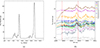 |
Fig. 1. Single-dish iMet monitoring data for the 6.7 GHz methanol maser in G11.497-1.485. (a) Averaged spectrum for MJD=60000-60250. (b) Light curve of the current maser flare. The flux density scale is logarithmic. The first noted flare took place on May 20, 2023 (60084 MJD); the maximum of the flare was detected on July 7, 2023 (60132 MJD). Two dotted red lines indicate the dates of the presented VLA observations (April 6 and July 18, 2023). |
In this paper we present the first high-resolution images of the centimeter continuum and masers obtained for G11.497-1.485 with the VLA. We aim to provide an overview of radio emission in the region and, by comparing the data from the two observations made during the current methanol maser flare, to evaluate if the recent maser activity is indicative of an accretion burst in the source or in the region. However, we emphasise that the final conclusion on the presence of an accretion burst will be based on the IR data that have recently been obtained for the region and will be published in Caratti o Garatti et al. (in prep.)
2. Observations and data reduction
Two triggered observing sessions (project code 23A-128) were conducted for G11.497-1.485 with the VLA: Epoch I was carried out on April 6, 2023, in B configuration, in response to the 6.7 GHz methanol flare (well before the first maximum (see Fig. 1); Epoch II was carried out on July 18, 2023 (close to the second maximum peak, Fig. 1) in A configuration. The same calibrator sources were used in both experiments: 3C286 as the delay, flux, and bandpass calibrator, and J1820-2528 as the phase reference source.
Continuum and spectral lines were observed in the C, Ku, and K bands during both VLA sessions. Parameters of the continuum and maser observations are listed in Tables 1 and 2. Table 2 also contains the list of the spectral line detection and non-detections. Continuum was observed in 31 spectral windows with 128 channels of 1000 kHz in each band and each epoch. Masers were observed in separate spectral windows of 1024 channels, except the C- and Ku-band masers at Epoch I, which were observed in 512 channels (see Table 2 for spectral resolution in each band).
Observation parameters: Continuum.
Observation parameters: Spectral line.
The Common Astronomy Software Applications (CASA5; CASA Team et al. 2022) was used for data reduction. We used the VLA CASA Calibration Pipeline for the initial data calibration. Then, the calibrated data were imaged with the CASA task tclean using natural weighting for continuum data and Briggs weighting for maser data. Gaussian fitting of the images was performed with the CASA task imfit. A two-dimensional Gaussian brightness distribution was fit to all continuum and maser emission peaks with a flux density above 3σ (see Tables 1 and 2 for the 1σ levels). The parameters of the detected continuum peak and maser spots are listed in Tables 3–4 and Tables A.1–A.6, respectively. It should be noted that here we present results for ‘maser spots’ – maser emission detected in a single velocity channel of a data cube. The maser spectra were obtained with the CASA Spectral Profile Tool.
Parameters of the detected continuum peaks.
Parameters of the components of the A configuration 1.3 cm continuum image of CM1.
Since the two epochs of observations were carried out with different VLA configurations (Epoch I in B configuration and Epoch II in A configuration), and thus with different angular resolution (Tables 1 and 2), we performed additional analysis to ensure a correct comparison of the data from the two epochs. The continuum emission appeared to be partly resolved with the obtained VLA resolutions. To compare the centimetre-continuum flux densities of the source at Epoch I and II in each band, we prepared the Epoch II images with limited uv ranges. In each band, we took the maximum uv range of the Epoch I image (B configuration) and set it as the cut level for the uv range of the Epoch II image (A configuration). The uv ranges and resulting normalised flux densities are listed in Table 3. The maser data, in contrast, are unresolved, even with the VLA A configuration. To verify it, we analysed the amplitude versus baseline length plots for the maximum intensity channel of the 6.7 GHz methanol data for each epoch. The plots showed no indication of the flux density decrease with uv distance. Additionally, we compared our VLA 6.7 GHz methanol maser spectra with the single-dish spectra obtained on the days of the VLA observations with the Hitachi 32 m radio telescope in the framework of the iMet programme; the single-dish and VLA spectra demonstrated the same (within uncertainties) flux densities at both epochs, confirming that the methanol maser emission is unresolved with the VLA resolution. The analysis for the 12 GHz and 22 GHz masers showed the same result – the emission is unresolved with the achieved VLA resolutions.
3. Results
Our VLA observations reveal four centimetre-continuum sources (CM1–CM4) and three loci of maser emission in the G11.497-1.485 region (see Fig. 2). CM1 is a centimetre-continuum source (Table 3) associated with strong 6.7 GHz (Table A.1), 12 GHz methanol (Table A.2), and 22 GHz water (Table A.3) masers. CM2 is a double-structure centimetre-continuum source (Table 3) that shows no maser emission and is located ∼7″ (∼9000 au at the distance of 1.25 kpc) to the north-east of CM1. CM3 is a centimetre-continuum source (Table 3) that shows no maser emission and is located ∼24″ (∼30 000 au) to the south-west of CM1. CM4 is a centimetre-continuum source (Table 3) with a 22 GHz water maser (< 20 Jy; Table A.4) located ∼7″ (∼9000 au) to the north-east of CM1. Finally, N is a source of weak 6.7 GHz methanol (< 1 Jy; Table A.5) and 22 GHz water masers (∼2 Jy; Table A.6) without an associated centimetre continuum, located ∼11″ (∼14 000 au) to the north of CM1. We present the results for all detected objects, but focus on CM1 because the flare of the 6.7 GHz methanol maser reported by the M2O is associated with this source.
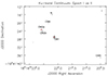 |
Fig. 2. Overview of the centimetre-continuum in G11.497-1.485: an overlay of the Epoch I (black contours) and II (red contours) Ku-band continuum images of the same uv range. Levels are [0.2, 0.4, 0.6, 0.8, 1] × 0.2 mJy beam−1. The positions of the N source without centimetre-continuum emission but with 6.7 GHz methanol and 22 GHz water masers only is indicated with a cross. See Table 1 for the synthesised beam sizes. |
3.1. Continuum
CM1. The continuum emission towards CM1 pinpoints a single, unresolved source with a flux density of a few hundred μJy (Table 3 and Fig. 3). The structure of the source starts to be resolved only in the K band with the A configuration (Epoch II; see Fig. 4 and Table 4 for the source components). Apart from the central source (‘Core component)’, the Epoch II K-band image shows an extended region (∼0.3″) of continuum emission to the north-west (‘NW component’) and a compact region of weak (∼50 μJy – 3σ level for our Epoch II K-band image) emission to the south (‘S component’). The core and NW components show similar peak flux densities of ∼110 μJy beam−1, although the NW component is more extended and has a higher integrated flux. Overall the region demonstrates the north–south orientation with both the core and NW components having a similar orientation with the positional angle of ∼40°. The southern component becomes a point source with the Epoch II K-band synthesised beam.
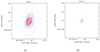 |
Fig. 3. Full uv-range continuum images of CM1 obtained at Epoch I (a) and Epoch II (b). Grey contours show the C band ([0.5–3] at Epoch I and [0.5–2] at Epoch II), blue the Ku band ([0.5–3.5] at Epoch I and [0.5–1.5] at Epoch II), and red the K band ([1–6.5] at Epoch I and [0.5–1] at Epoch II). Levels are of ×0.1 mJy beam−1 with the 0.5 step. See Table 1 for the synthesised beam sizes. |
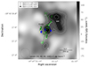 |
Fig. 4. 1.3 cm continuum image and masers detected at Epoch II towards CM1. Each continuum component of CM1 is labelled, and different types of masers are marked by colour (see the legend). |
To compare the flux densities of CM1 in different bands and epochs, we prepared the images with restricted uv range (see Section 2 for details). As a common uv range, we chose the Epoch II Ku-band value (313 kλ; Table 1) since it provided a sufficient resolution and we were forced to exclude only the Epoch I C-band data, which had a twice shorter uv range. Using the obtained normalised flux densities listed in Table 3, we plotted a flux density versus frequency graph (see Fig. 5a). We note that since the source is unresolved with the vast majority of our data, we analysed the accumulative flux density of the region without discrimination between the components identified in the Epoch II K-band image (Table 4). The flux density of the source appeared to steadily rise with frequency (Fig. 5a), showing a spectral index of ∼0.4. The positive spectral index is consistent with emission arising from a thermal radio jet or an ultracompact to hyper-compact HII region, although the obtained data do not allow us to definitively conclude on the nature of the source.
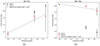 |
Fig. 5. Flux density–frequency dependence for the centimetre-continuum sources CM1 (a) and CM2a (b). The filled circles with error bars represent the normalised integrated flux densities with errors from Table 3 (black for Epoch I and red for Epoch II). The presented flux density values were obtained using the uv range of 1–313 kλ (for details, see the text of Sect. 2). |
Epoch II uv-cut images report ∼×1.2 lower values of the flux density for CM1 (Table 3); however, the difference between fluxes is within the uncertainties (see Fig. 5a). We consider the lower flux densities to be caused by partial resolving of the source in a higher-resolution observation at Epoch II.
CM2. A double-structure centimetre-continuum source CM2 is found at ∼7″ (∼9000 au) separation from CM1 (Fig. 2). We note that for the au-scale estimation, we assumed the distance of 1.25 kpc, which was established by the 12 GHz methanol maser parallaxes in CM1 (Wu et al. 2014), namely we assume that CM1 and CM2 (as well as other sources that we discuss below) are located in the same region. Brightening of centimetre-continuum emission in CM2 was detected at Epoch II (Table 3 and Fig. 6). At Epoch I, the source showed two continuum peaks, which we labelled CM2a and b. CM2b is found to the south-west of CM2a, and the sources are separated by ∼0.8″ (or 1000 au). CM2a and CM2b showed similar flux densities of ∼100 μJy at Epoch I, but by Epoch II, CM2a reached a flux of ∼500 μJy and CM2b remained detectable only in the C band. One more weak component (< 90 μJy), CM2c, located ∼1.5″ (1900 au) away from CM2a, was detected at Epoch I only.
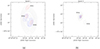 |
Fig. 6. Full uv-range continuum images of CM2 obtained at Epoch I (a) and Epoch II (b). Grey contours represent the C band ([0.6–2.6] at Epoch I and [1–6] at Epoch II), blue the Ku band ([0.6–1.4] at Epoch I and [1–5] at Epoch II), and red the K band ([0.6–1] at Epoch I and [1–5] at Epoch II). Levels are of ×0.1 mJy beam−1 with the 0.2 step for Epoch I and 0.5 step for Epoch II. See Table 1 for the synthesised beam sizes. |
Following the same procedure we used for CM1, we estimated the normalised flux densities for CM2 (Table 3) using the restricted uv-range images. The comparison of the normalised fluxes obtained at each epoch reported a factor of 5 increase for CM2a and at least a factor of 3 decrease for CM2b (considering the 3σ level as the detection threshold for CM2b; see Table 3). The flux density versus frequency graph for CM2a is presented in Fig.5b. The flux density of CM2a falls with frequency (Fig. 5b), showing a negative spectral index of ∼ − 0.3. The detected strong variability coupled with the negative spectral index suggests that the centimetre-continuum emission of CM2 may be non-thermal (synchrotron). We note that the source was present in the VLA C-configuration 8.4 GHz image from van der Walt et al. (2003), but the parameters of the source were not reported.
CM3. Out of all other centimetre-continuum sources found in the region, CM3 is found at the maximum separation (> 20″ or ∼30 000 au) from CM1. At Epoch I, the source shows weak emission of ∼90 μJy in the C and Ku bands, while the highest-frequency image obtained in the K band reported a non-detection (Fig. 7a). At Epoch II, no sign of the source emission is found in either band. We refrain from judging the spectral index of the source as we obtained only two flux measurements. However, we note that the flux density of CM3 is about the same (within uncertainties) in the C and Ku bands, suggesting that the spectral index might be flat or at least not very steep.
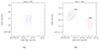 |
Fig. 7. Full uv-range continuum images of CM3 (a) and CM4 (b) obtained at Epoch I (non-detection at Epoch II for both sources). Levels are [0.3, 0.5, 0.7, 0.9, 1.1] × 0.1 mJy. Grey contours represent the C band, blue the Ku band, and red the K band. See Table 1 for the synthesised beam sizes. |
The position of CM3 coincides with the first of two H2 knots reported by De Buizer (2003). Thus, the centimetre-continuum emission is most probably associated with the large-scale outflow from CM1. Considering the linear distribution of the sources CM2, CM1, and CM3, we suggest that CM2 and CM3 mark the radio-lobes of the outflow from CM1.
CM4. The K-band Epoch I image revealed the double structure of the source with two components, denoted as CM4a and CM4b, separated by 1.7″ or ∼2000 au (Fig. 7b). However, the component CM4b is not detected in any other band or epoch. The source CM4a showed a non-detection in the C band, a 6σ detection in the Ku band, and the flux density of ∼200 μJy in the K band. The detected increase in flux density with frequency for CM4a hints at the presence of a thermal jet and/or (UC)HII region.
3.2. 6.7 GHz methanol maser
CM1. The 6.7 GHz class II methanol maser emission towards CM1 is detected at both epochs in the velocity range ∼4–18 km s−1 (Fig. 8a). Two groups of the spectral features can be identified: the group with the blueshifted velocities occupies the range ∼4–10 km s−1 with the peak at ∼8.3 km s−1, and the group with the redshifted velocities occupies the range ∼12–18 km s−1 with the peak at ∼16.8 km s−1. Notably, the two velocity groups are almost symmetrical with respect to the systemic velocity of the source VLSR = 10.74 km s−1 (Liu et al. 2016); they show the same velocity extent (∼6 km s−1), similar spectral profile and number of features, and the peak at the high-velocity end of the group.
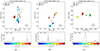 |
Fig. 8. Combined Epoch I and II VLA spot maps of the 6.7 GHz methanol maser (a), the 12 GHz methanol maser (b), and the 22 GHz water maser (c) in CM1. Maser spots are coloured by velocity. The dotted grey line in the spot maps indicates the orientation of the large-scale outflow identified by the H2 knots in De Buizer (2003). The dotted grey line in the spectra indicates the systemic velocity of the source (VLSR = 10.74 km s−1; Liu et al. 2016). |
The spectra detected at Epoch I and II present the same spectral features over the same velocity range (Fig. 8a). The most striking change between the epochs is that the spectral feature with the maximum redshifted VLSR = 16.8 km s−1 became dominant in the spectrum, while at the previous VLA epoch the spectral feature with the maximum blueshifted VLSR = 8.3 km s−1 was dominant. The flux of the redshifted spectral feature at VLSR = 16.8 km s−1 increased ∼2.6 times between the two VLA observations. While the flux density of the blueshifted peak, which flared initially, remained stable. If we inspect the weaker spectral features (see Fig. 9), we see that almost all of them have increased flux density (by a factor of ∼1.3), with the most profound change in the blueshifted feature at VLSR = 7.4 km s−1 (the one preceding the dominant blueshifted feature at VLSR = 8.3 km s−1), which showed ∼×2.9 higher flux. However, two features with minimal blueshifted velocities (VLSR = 5.3 and 5.8 km s−1) show the same flux at both epochs.
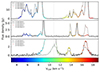 |
Fig. 9. Close up on the flux density variation in the weak spectral features of the maser emission associated with CM1. The dotted grey line indicates the systemic velocity of the source (VLSR = 10.74 km s−1; Liu et al. 2016). |
The detected 6.7 GHz methanol maser spots are found in a region of ∼0.5″ × 0.2″ (600 au × 250 au at the distance of 1.25 kpc), eastwards of the continuum peak CM1 (Fig. 8a). We note that, in the presented spot maps, we use the coordinates of the Core component of CM1 (Table 4), which indicates the central source, but does not pinpoint its exact position as the K-band continuum is most probably contaminated by the ejection from the source (the continuum shows a slight extent in the NE-SW direction in Fig. 4). Therefore, the obtained positional uncertainty amounts to ±0.01″ (Table 4), thus positioning of CM1 at the eastern edge of the 6.7 GHz methanol maser distribution might be an imaging issue. The 6.7 GHz methanol maser emission is associated with the core component of the continuum emission but seem to evade the regions of the NW and S components (Fig. 4). Notably the 6.7 GHz methanol maser spots cross beyond the core continuum component only in the north-eastern part of the region but not in the south-western, which is bounded by the NW and S components. The maser spots trace curved strings of maser emission elongated in the north-south direction (Fig. 8a). As with the spectra, the two velocity groups are clearly distinguishable and show some symmetry in the spot map. While the spots with the blueshifted velocities stretch out in the N–S direction, the redshifted spots show the NW–SE orientation and cross the blue-velocity strings near the position of the 1.3 cm continuum peak. The elongated strings of spots are mostly traced by the weak (< 15 Jy) emission, while the emission of the dominant spectral features comes from more compact clusters. The maser spots with the extreme blueshifted (VLSR = ∼8.3 km s−1) and redshifted (VLSR ∼ 16.8 km s−1) velocities form two symmetrically oriented clusters separated by ∼0.1″ (125 au) and having the same size of ∼0.07″ (90 au).
Comparison of the maser spot maps obtained at Epochs I and II (Figs. 8a and 10) shows the expected brightening of the cluster with the peak redshifted velocities. Apart from that, a new string of the blueshifted maser spots associated with brightening of the spectral feature at VLSR ∼ 7.4 km s−1 appeared in the north.
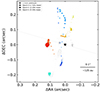 |
Fig. 10. CM1 6.7 GHz methanol maser spots that showed increased fluxes during Epoch II (coloured by velocity) compared to Epoch I. The dotted grey line indicates the orientation of the large-scale outflow identified by the H2 knots in De Buizer (2003). |
N. The 6.7 GHz methanol maser emission towards the N source is detected at both epochs in the velocity range ∼12–14 km s−1 (Fig. 11b). The spectrum consists of one blended spectral feature with the peak VLSR = 13 km s−1 and flux density ∼0.5 Jy. The spectral feature showed a little lower flux density at Epoch II but the difference was close to the flux density scale uncertainty.
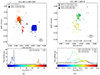 |
Fig. 11. Spot maps and spectra of the maser emission detected towards the sources CM4 (a) and N (b) at Epochs I and II. |
The spatial distribution of the 6.7 GHz methanol maser spots resembles a circular structure with offshoots to the north-east and south-west. However, we note that the low flux density of the maser emission (∼0.5 Jy) does not allow for precise position estimation (see the uncertainties in Table A.5) and any apparent patterns should be treated with caution. Considering the 1.25 kpc distance, the 6.7 GHz maser emission covers a region of ∼50 au (∼0.04″) while the ring-like structure has the size of only ∼13 au (∼0.01″).
3.3. 12 GHz methanol maser
In contrast to the 6.7 GHz methanol and 22 GHz water masers, the 12 GHz methanol maser emission is not detected in any other source in the region except CM1. The spectral profile of the 12 GHz methanol maser in the source is similar to the 6.7 GHz methanol maser profile with similar spectral features appearing almost at the same velocities (Fig. 8b). The 12 GHz methanol maser emission is detected at both epochs in the velocity range of ∼5–18 km s−1, consisting of two distinct spectral feature groups with blue- and redshifted velocities. However, the flux density of the 12 GHz maser is lower, with the brightest feature reaching ∼15 Jy while the 6.7 GHz maser shows flux densities ∼100 Jy. The strongest 12 GHz maser feature with VLSR = 8.9 km s−1 dominates the group with blueshifted velocities (as in the 6.7 GHz spectra) while the group with redshifted velocities is dominated by the feature with VLSR = 15.1 km s−1 at Epoch I and shows almost equal fluxes for the three spectral features constituting the group at Epoch II.
In contrast to the 6.7 GHz methanol maser, in the 12 GHz maser, the most noticeable increase in flux density6 happened not only in the spectral feature with the maximum redshifted velocity 16.6 km s−1, but also in the dominant feature of the blue spectral group (VLSR = 8.9 km s−1) and the spectral feature with the minimum redshifted velocity (VLSR = 13.8 km s−1) (Figs. 8b and 9). The flux density change amounted to ×1.6 for the VLSR = 8.9 km s−1 feature, ×2.3 for VLSR = 13.8 km s−1, and ×5.3 for VLSR = 16.6 km s−1. As in the case of the 6.7 GHz methanol maser spectra, some degree of flux change is noticeable for almost all spectral features (Fig. 9), with the only exception of the blueshifted feature with VLSR = 5.8 km s−1.
The 12 GHz methanol maser emission occupies a region of about the same size as the 6.7 GHz methanol maser; however, the lower flux density of the 12 GHz methanol maser restricted the number of detected maser spots (Fig. 8b). Similarly to the 6.7 GHz masers, the 12 GHz masers are associated with the core continuum component only (Fig. 4). The 12 GHz methanol maser spots with the redshifted velocities are found in the north of the masering region and the spots with blueshifted velocities are found in the south. The 12 GHz masers trace the same structures as the 6.7 GHz masers, with the exception of the northern blueshifted spots, which are not detected at 12 GHz. The brightest 12 GHz methanol maser emission highlights the southernmost edge of the masering region. The 12 GHz masers are overall found at greater separations from the central source compared to the corresponding 6.7 GHz maser clusters (Fig. 8). This behaviour is in accordance with the theoretical works for 12 GHz methanol maser pumping; the 12 GHz methanol masers are known to require a very similar environment as 6.7 GHz masers but over a narrower range of physical parameters of gas (Cragg et al. 2005). For instance, 12 GHz methanol masers decay faster than the 6.7 GHz masers with increasing gas temperature. Thus, the 12 GHz methanol masers trace the regions of lower temperatures that are found at greater separations from the central source.
Similarly to the 6.7 GHz methanol maser, the comparison of the Epoch I and II spot maps for the 12 GHz methanol maser showed brightening of the eastern cluster of the spots with the redshifted velocities (Figs. 8b and 10). Additionally, at Epoch II, the southernmost cluster of the spots with the blueshifted velocities (VLSR = 8.9 km s−1) experienced an increased flux density; in this part of the masering region, a string of weak 6.7 GHz methanol maser appeared at Epoch II. Another cluster showing an increased flux at Epoch II is the ‘yellow’ cluster to the north-west of the position of the 1.3 cm continuum peak. Notably a couple of weak 12 GHz maser spots with blueshifted velocities appeared at Epoch II in the northern edge of the region, at the end of the new string of the 6.7 GHz methanol masers.
3.4. 22 GHz water maser
CM1. At both epochs, the 22 GHz water maser emission is detected in the VLSR-range from ∼8 km s−1 to ∼18 km s−1 (Fig. 8c), that is to say, in a range ∼4 km s−1 shorter than the methanol masers that have the features at the velocities starting from ∼4 km s−1. In the 22 GHz water maser spectra, three maser features can be distinguished: ‘green’ with the VLSR close to the systemic velocity 10.74 km s−1, yellow with the VLSR = ∼ 13.6 km s−1, and ‘red’ with the redshifted velocities of ∼16.6 km s−1.
The spatial distribution of the 22 GHz water maser spots (Fig. 8c) is quite different compared to the methanol maser distribution and occupies a region of ∼0.2″ (250 au) linearly extended in the east-west direction. The water maser spots form three compact (∼0.02″ or 30 au) clusters with distinct velocities: the clusters with the green and redshifted velocities straddle the 1.3 cm continuum peak at about equal separations of ∼0.05″ (70 au) to the west and east, respectively; while the yellow cluster is separated by 0.1″ (125 au) to the east from the continuum peak (see Fig. 4). Notably the water maser clusters are distributed perpendicularly to the extent of the methanol maser emission but parallel to the axis of the proposed large-scale H2 outflow (De Buizer 2003), which suggests an association of the 22 GHz water masers with the outflow.
In contrast to the methanol masers, the water emission has dimmed by Epoch II (Figs. 8c and 9). The most profound change is noticeable for the green spectral feature, whose flux density has dropped by ∼6 times and the width has shrunken by ∼2 times. The yellow and red features underwent a less dramatic transformation; their flux density declined by ∼1.5 times. We note that the 22 GHz water maser flare that the M2O reported originated from the CM4 source and not the central source.
The spot map obtained at Epoch II shows no change in the overall distribution of the 22 GHz water maser emission (Fig. 8c), although the dimming of the flux density results in few maser spots being detected. The water maser clusters appear to be spatially more compact at Epoch II, and with slightly smaller velocity ranges.. This is especially apparent for the green cluster, which does not show the most extreme blueshifted velocities that were present in Epoch I (Fig. 9).
CM4. The 22 GHz water masers associated with CM4 are found in the velocity range from −3.5 to 25.5 s−1 (Fig. 11a and Table A.4). The spectrum consists of two distinct spectral groups with blueshifted (VLSR = −3.5–0.5 km s−1) and redshifted spectral features (VLSR = 18.6–25.5 km s−1). The blueshifted velocity features are blended while the redshifted velocity group shows one dominant peak.
Between the two epochs of observations, an increase in the flux density of the water maser in CM4 occurred. The maximum flux density of the blueshifted group increased ∼10 times (from ∼1.8 Jy to ∼18.7 Jy) and of the redshifted group – ∼2 times (from ∼3 Jy to ∼6.8 Jy). Notably, the peak velocity of both velocity groups also changed. The peak velocity of the blue group changed from VLSR = −1.26 km s−1 to −0.63 km s−1 (ΔV = 0.63 km s−1), and the peak velocity of the red group shifted from VLSR = 19.33 km s−1 to 20.28 km s−1 (ΔV = 0.95 km s−1).
The masers with the blue- and redshifted velocities can be clearly distinguished not only in the spectrum but also in the spot map (Fig. 11). The two velocity groups are associated with two compact maser clusters, oriented to the NE–SW relative to each other, and separated by ∼0.06″ (or 75 au considering the 1.25 kpc distance). At Epoch II, a cluster of weak emission (∼0.5 Jy) corresponding to the spectral feature at VLSR ∼ 25 km s−1 is found about 0.03″ (35 au) to the south of the red cluster. This velocity component is associated with the CM4a continuum source, and the mutual orientation of the components CM4a and CM4b closely resembles that of the blue- and red-lobe of the water maser.
A shift in the position of the red spatial cluster is noted at Epoch II. The geometric centre of the red cluster moved < 0.01″ (∼13 au) in the north-eastern direction while the blue cluster remained in place (within uncertainties). A displacement of 13 au during the 3.5 months separating Epochs I and II suggests a velocity of the order of 200 km s−1 (ignoring inclination effects). Such a velocity is consistent with a jet interpretation for CM4, although in this scenario we would expect a similar displacement in the blueshifted maser cluster, which is not seen. However, there are other possibilities, for example that the two lobes have different velocities, propagating in a differently dense environment. The spots with velocities of ∼25 km s−1, in turn, shifted to the west, but we note that this movement is less reliable as the flux density of the cluster is low (∼0.5 Jy) and, consequently, positional uncertainties are high.
N. The spectrum of the 22 GHz water maser associated with the N source consists of one weak (∼2 Jy) spectral feature at VLSR ∼ 12 km s−1 (Fig. 11b and Table A.6). Comparison between the two epochs of observation showed a ×2.5 fading of the water maser emission in the source.
The 22 GHz water maser spots form a compact cluster located ∼0.03″ (∼40 au) to the north of the centre of the 6.7 GHz methanol maser cluster. The 22 GHz water maser cluster did not show any positional shift between the epochs.
4. Discussion
4.1. Structure of the G11.497-1.485 region
As noted in Sect. 1, the G11.497-1.485 region has been featured in a number of surveys but lacked more detailed information. Previous observation of the region reported the results only for the most active source – CM1 (e.g. De Buizer 2003; van der Walt et al. 2003; Hu et al. 2016). Our VLA observations revealed for the first time that the region hosts at least five distinct radio sources (Fig. 2). The obtained data enable us to speculate on the nature of each source.
Since 6.7 GHz methanol masers are known to be associated with high-mass star formation (e.g. Minier et al. 2003), we consider the sources CM1 and N to be MYSOs. The identified massive protostars, CM1 and N, also show 22 GHz water maser emission that is associated with shocked regions and trace ejection (e.g. Cesaroni et al. 2013; Gray et al. 2022). In CM4, the 22 GHz water maser spectrum resembles a high velocity jet and therefore is likely associated with either a MYSO or an evolved star. The increase in the CM4 continuum flux density with frequency also argues in favour of its association with an HII region and/or thermal jet.
The positions of the centimetre-continuum sources CM2 and CM3, found to the north-east and south-west of CM1, respectively, match the orientation of the SO-outflow reported by De Buizer et al. (2009). The negative spectral index and high variability of the centimetre continuum from CM2 suggest that the emission can have non-thermal nature and be associated with synchrotron knot of the radio jet, similar to the cases detected for massive protostars recently in, for example, Moscadelli et al. (2013, 2016). Strong evidence in favour of CM3 marking ejection is the fact that it coincides with an H2 knot detected in De Buizer (2003). Notably, CM2 and CM3 are offset to the north from the axis of the jet. Such a placement of non-thermal knots has been noted for low-mass stars, and these knots have been explained as deflection shocks, namely (quasi-)stationary shocks at the working surfaces where the jet hits the dense ambient material (Hartigan et al. 2005; Purser et al. 2018). Additionally, deflection shocks have been noted to show the linear morphology perpendicular to the jet axis (Hartigan et al. 2005; Purser et al. 2018), similar to the morphology of the CM2a source in the K-band Epoch II image (Fig. 6b; i.e. the highest resolution image of the source). In the case of the stationary shock scenario, no significant proper motions for CM2 and CM3 is expected to be observed and it seems to be supported by the fact that CM3 and the H2 knot detected in 2003 arise from the same location, although the coordinates of the H2 knot were not reported in De Buizer (2003) and we cannot estimate the precise numerical value of the offset between the radio and H2 knots.
One peculiar feature of the G11.497-1.485 region is the very small sizes of the maser clusters in the CM4 and N sources. The water masers in CM4 are separated by ∼0.06″ or ∼75 au, and the 6.7 GHz methanol – 22 GHz water maser system in N has the size of ∼0.04″ or ∼50 au. While the most compact outflows traced by water masers has size of ∼180 au (Torrelles et al. 2014) and accretion discs around massive stars traced by 6.7 GHz methanol masers typically have sizes of a few hundred au. Thus, the maser traced systems detected in CM4 and N are one of the most compact ones found to date. A possible explanation of such compact sizes is that the water masers in these sources arise within the circumstellar environment, as was proposed, for example, for Ceph A HW2 in Torrelles et al. (1996). Another possibility is that CM4 and N are in fact background sources. We note that the distance of 1.25 kpc to the G11.497-1.485 source was estimated by the parallax observations of the 12 GHz methanol maser in CM1 (Wu et al. 2014), consequently we can confidently apply the distance estimate to this source only.
4.2. Disc fragmentation in CM1
Methanol masers at 6.7 GHz and 12 GHz are known to trace accretion discs around massive stars (e.g. de Buizer et al. 2000; Cesaroni et al. 2013). The configuration of the methanol masers in G11.497-1.485 CM1 seems to fit into this scenario as the masers are symmetrically distributed around the central continuum source with inclination perpendicular to the large-scale outflow (Figs. 8a,b). If we consider the 6.7 GHz and 12 GHz methanol masers to trace an accretion disc around CM1, we can assume that the disc has a diameter of ∼625 au (the total size of the N-S methanol maser distribution of ∼0.5″ at the distance of 1.25 kpc; Fig. 12) and the inclination angle relative to the observer’s line of sight of ∼75° (from the relation between the semi-major and semi-minor axes of the elliptical maser region). Although methanol masers do not trace the most dense parts of the disc mid-plane as they are quenched at the hydrogen number densities exceeding 108–109 cm−3 (Meyer et al. 2018). We attempted to model the 6.7 GHz methanol maser data (we considered only the maser spots with the positional uncertainties of < 5 mas; see Table A.1) using the minimum chi-square method described in Moscadelli et al. (2019) but the estimate reported a non-Keplerian velocity profile for the dataset.
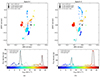 |
Fig. 12. Comparison of the Epoch I and II maser spatial distribution. Maser spots are coloured by velocity. |
The methanol maser spots show a ‘string-like’ morphology, with emission at particular velocities extending in the NS direction. This morphology may partly result from the low angular resolution of our observations and the approach of fitting maser ‘spots’. In particular, distinct channels of a single velocity feature maser can trace spatial structure at angular scales smaller than the intrinsic angular resolution of the observations. The linear N–S patterns of the maser spots are also seen in the lower-resolution VLA C-configuration image from Hu et al. (2016) and in the higher resolution VLBI image of Fujisawa et al. (2014); hence, we consider this to be a robust feature. We assume that with the obtained VLA data we start to access the coherent physical structure of an accretion disc in G11.497-1.485. The high flux densities of the flaring masers in conjunction with usage of the VLBI heatwave mapping method revealed the presence of spiral arms in the accretion disc of G358.93-0.03 (Burns et al. 2023). However, hints to the presence of the spiral arms in G358.93-0.03 had been already noted in lower-resolution VLA observations (Chen et al. 2020; Bayandina et al. 2022b). The distance to G358.93-0.03 is ∼6.75 kpc (according to the BeSSeL Revised Kinematic Distance Calculator; Reid et al. 2014), while G11.497-1.485 is located almost five times closer. Thus, we can start resolving the disc using a lower resolution.
The VLA A-configuration 1.3 cm continuum image has revealed the fine structure of CM1 (Fig. 4) for the first time. Apart from the Core continuum component, the K-band Epoch II image (Fig. 4) also shows another two peaks – NW and S. Interestingly, the NW and S centimetre-continuum components are found at the edges of the methanol maser cluster. The continuum peaks might mark the sites of disc fragmentation, namely the clumps of high density (∼10−11 g cm−3, ∼100 times denser than spiral arms and ∼10 000 denser than background accretion disc) and high temperature (∼600 K) (Oliva & Kuiper 2020) in the spiral arms traced by the 6.7 GHz methanol masers. Since the Core and NW continuum emission peaks have very similar flux densities and the NW component has an extended spatial structure, the NW component may be a fragment forming a second core with a potential secondary disc (e.g. Oliva & Kuiper 2020). On the other hand, the S component seems to be a less developed fragment or a fragment that was drained by a spiral arm transporting matter from the fragment to the central protostar (Oliva & Kuiper 2020). Fragmentation of accretion disc is crucial in formation of massive stars; accretion discs around massive stars form spiral arms that fragment further. The fragments can either be accreted onto the central protostar through the spiral arms or form companion protostellar cores (Oliva & Kuiper 2020). This mechanism is modelled in a few theoretical works (Meyer et al. 2018; Oliva & Kuiper 2020), and the fragments are thought to be detected in a few individual objects (e.g. Ilee et al. 2018; Johnston et al. 2020). Remarkably, if our assumption about the nature of the continuum peaks is correct, G11.497-1.485 CM1 would set the example of the most compact fragmenting system, as the NW and S components are found at the separations of ∼300 au from the central object, while all the previous sightings of fragments in massive protostars reported separations of ∼1000 au (Sanna et al. 2015; Beuther et al. 2017; Hunter et al. 2017; Ilee et al. 2018; Johnston et al. 2020).
4.3. Methanol maser flare in CM1 – Accretion burst evidence?
The G11.497-1.485 region is known to show quite variable 6.7 GHz methanol and 22 GHz water maser emission; however, the nature of the maser flares in the source has never been studied in detail. According to the list of articles collected in MaserDB7, the 6.7 GHz methanol maser was in a high-activity state in the 1990s with the flux density ≳100 Jy (Gaylard et al. 1994; Walsh et al. 1997, 1998; Szymczak et al. 2000), and the record flux of ∼248 Jy achieved in May-July 1992 (Schutte et al. 1993). In contrast, in the 2000–2010 s, the 6.7 GHz methanol maser showed the flux densities at a median level of only ∼65 Jy (Szymczak et al. 2012; Vlemmings et al. 2011; Fujisawa et al. 2014; Hu et al. 2016), with the highest value being ∼107 Jy in an observation from 2003 (Fontani et al. 2010).
However, the most peculiar characteristic of all these observations is the fact that in all of them the dominant spectral feature was at VLSR = ∼ 6.5 km s−1, where we now see no strong emission in our VLA observations. Instead, the dominant spectral features are found at redder velocities of VLSR = ∼ 8.3 km s−1 at Epoch I and VLSR = ∼ 16.8 km s−1 at Epoch II (Fig. 8a). The change of the dominant spectral feature must be associated with a physical change in the source.
The 6.7 GHz methanol maser clusters associated with the dominant spectral features have always been found to the south of the continuum peak, for example the L cluster from Walsh et al. (1998), the maser spots at the (0, 0) position in Hu et al. (2016) and Fujisawa et al. (2014), the turquoise cluster that was dominant in the spectrum at our Epoch I, and the red cluster that was dominant at our Epoch II (see Fig. 8a). The change of the dominant spectral feature has a clear velocity and spatial pattern: the velocity of peak intensity has changed from the least blue to the most red, and the brightest maser cluster is no longer the southern one but rather the red cluster located east of the continuum peak. Noteworthy is the general NE-SW orientation of the brightest clusters, which is similar to the orientation of the large-scale outflow (Fig. 8a).
If we look at the distribution of the maser spots that flared at Epoch II (see Fig. 10), we can see that the spots with increased fluxes are found at the edges of the region. The turquoise 12 GHz methanol maser cluster (VLSR = 9 km s−1) at the edge of the region brightened, while the 6.7 GHz methanol maser cluster with similar velocities but located closer to the central source showed no change in flux. Apart from it, the ‘orange’ (VLSR = 15 km s−1) cluster of the 12 GHz methanol maser emission demonstrated stable flux during Epoch I and II, but the yellow (VLSR = 13.8 km s−1) 12 GHz methanol maser cluster located in the same direction to the north-west of the central source but at a greater separation (∼0.1″ or ∼125 au) showed an increased flux at Epoch II. Finally, only the lowest edge of the blue cluster (VLSR = 4–7 km s−1) to the south of the central source flared in 6.7 GHz and 12 GHz maser emission, while the flux density of the innermost part of the cluster remained stable over Epoch I and II. One region that demonstrated equally strong brightening both in 6.7 GHz and 12 GHz methanol maser emission is the easternmost cluster with the redshifted velocities of ∼16.8 km s−1. Within this cluster, the positions of the 6.7 GHz and 12 GHz masers agree well, though the 12 GHz methanol maser traces a more compact area. The most obvious change in the overall maser distribution is the appearance of a new string of the 6.7 GHz methanol maser emission in the northern part of the source. No 6.7 GHz methanol maser emission in this part of the region was detected at Epoch I, and the archival spot map from Hu et al. (2016) shows only a single line of 6.7 GHz masers in the northern part of the region. However, we note that the observations of Hu et al. (2016) were done with the VLA C configuration, which might have been insufficient to resolve two close strings of emission. Given the lack of strong evidence for the existence of this new structure at earlier epochs, we argue that it first emerged sometime between Epoch I and II.
Expansion of the masering region as well as appearance of new maser clusters were the key features of the accretion burst detected recently in G358.93-0.03 (e.g. Burns et al. 2020, 2023; Chen et al. 2020; Bayandina et al. 2022b). The heatwave of the accretion burst ignited radiatively pumped class II methanol masers at ever expanding radii providing us with the first opportunity to track the propagation of the energy of an accretion burst through the surrounding region using so-called ‘heatwave mapping’ (Burns et al. 2020). In the case of G11.497-1.485, we seem to witness a similar picture, the supposed propagation of the heatwave is indicated by stable fluxes of the innermost maser clusters and flaring or appearance of new clusters at the edges of the region at Epoch II.
Other evidence supporting the heatwave propagation theory for G11.497-1.485 CM1 is the fading of the 22 GHz water masers in the vicinity of the central source (Fig. 8). Water masers are pumped by collisions, but excessive radiation can block the sink transition and effectively quench the maser emission (Sobolev et al. 2019; Gray et al. 2022). Weakening or disappearance of water masers at 22 GHz was detected for previously discovered sources of accretion bursts (e.g. Brogan et al. 2018; Bayandina et al. 2022a). In G11.497-1.485, the most significant flux density drop at Epoch II is registered for the westernmost water maser (VLSR = 8–12 km s−1), which, similarly to the flaring masers, is found at an edge of the masering region. Thus, again, we can argue that the heatwave of a possible accretion burst reached the edges of the region sometime between Epoch I and II.
However, if there was an accretion burst in G11.497-1.485, it was of a low magnitude. In G11.497-1.485, we detected no fading of the centimetre continuum from the central source, which would have been expected because of the bloating of the protostar after accreting a fragment (e.g. Hosokawa & Omukai 2009) and decrease in the density and temperature of other fragments due to their thermal expansion triggered by the propagation of the burst heatwave through the disc (Oliva & Kuiper 2020). A decrease in the centimetre-continuum flux density was detected, for example, in the accretion burst sources G358.93-0.03 MM1 and NGC 6334I, where the continuum faded by a factor of > 5 (Bayandina et al. 2022b) and ∼5.4 (Brogan et al. 2018), correspondingly. Additionally, we detected no rare methanol masers (see the list of non-detections in Table 2), which were the distinctive characteristic of the accretion burst in G358.93-0.03 MM1 (MacLeod et al. 2019; Breen et al. 2019; Bayandina et al. 2022b).
4.4. Transient event in G11.497-1.485
In the period April-July 2023 (inclusive), that is, between epochs I and II of our VLA observation, all the detected sources of the region showed high activity. Apart from the flare of the 6.7 GHz methanol maser that initially triggered our study, CM1 also showed an increased flux of 12 GHz methanol maser, as well as dimming of 22 GHz water maser. CM2 showed a centimetre-continuum brightening while CM3 disappeared. The CM4 source showed a 22 GHz water maser and continuum emission brightening. And the 22 GHz water maser in the N source dimmed.
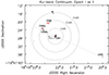 |
Fig. 13. Estimation of the propagation time of a light-speed disturbance in the region. |
Observations of 22 GHz water masers in G358.93-0.03 showed that an accretion burst can affect not only the immediate vicinity of a bursting protostar, but also neighbouring sources (Bayandina et al. 2022a). Radiation propagating with the speed of light would cover ∼5300 au in a month. Adopting this estimate, we prepared an approximate scheme of light propagation from CM1 into the G11.497-1.485 region (see Fig. 13). According to the scheme, the sources CM2 and CM4 would be affected in ∼2 month, the source N – in ∼3 month, and CM3 – in ∼6 month. The onset of the 6.7 GHz methanol maser flare and our first VLA observation took place in April 2023, the second VLA epoch was conducted 3.5 month later, in July 2023 (Fig. 1). We expect water masers to fade and methanol masers to flare upon arrival of radiation. After the region is radiated, the sink transition is no longer blocked and water masers show flares (e.g. Bayandina et al. 2022a). Thus, we can assume that by Epoch II the light echo has already left the CM4 source and the 22 GHz water masers flared, while the N source is still affected by the radiation and the 22 GHz water maser faded. However, the flare of the water maser in CM4 seems to be associated with the jet-lobe propagation (Fig. 11) and not with any external influence.
While the flare of the 6.7 GHz methanol maser in G11.497-1.485 was initially interpreted as a sign of an accretion burst and we indeed found some possible supporting evidence, our VLA data alone cannot confirm this interpretation and we ought to consider alternative scenarios. According to the single-dish monitoring data, the 6.7 GHz methanol maser in G11.497-1.485 started to show quasi-periodic flares after the initial flux rise in April 2023 (Fig. 1). Similar behaviour has been noted before for a handful of 6.7 GHz masers, such as G107.298+5.639 (Szymczak et al. 2016), G59.633-0.192 (Olech et al. 2019), G45.804-0.356 and G49.043-1.079 (Olech et al. 2022). The most plausible explanation for the detected quasi-periodic flares seems to be modulated accretion (i.e. instabilities in the accretion flow; e.g. Oliva & Kuiper 2020) or an interaction of the disc material with a second body (e.g. Araya et al. 2010; Parfenov & Sobolev 2014; van der Walt et al. 2016).
For the central source CM1, both the maser and continuum data suggest higher activity in the red lobe of the jet/outflow at Epoch II. As we have already pointed out, the distinctive characteristic of the 6.7 GHz methanol maser flare observed at Epoch II is the change of the dominant spectral peak from the blueshifted feature, seen in previous observations, to the redshifted feature (Fig. 8a), which started flaring for the first time in around May 2023 (Fig. 1). The brightest 6.7 GHz methanol maser clusters (VLSR = ∼ 6, 8, and 16 km s−1) are found in the south-west of the CM1 region and they roughly follow the orientation of the outflow (Fig. 8a); thus, the flare of the redshifted spectral feature at VLSR = ∼ 16.5 km s−1 could be associated with an ejection event. The detected brightening of the CM2 radio knot might then be connected to the same event and indicate an asymmetric mass-loss or ejection process (such cases were detected in low-mass young stellar objects; e.g. Purser et al. 2018).
Finally, as proposed by Liu et al. (2023) for the accretion burst candidate G24.33+0.14, periodic methanol maser flares could also be triggered by the radiation field of a nearby source rather than the central protostar itself. The VLA data presented here confirm that CM1 is the most active radio source in the region; however, we must wait for IR data to conclude on the trigger behind the methanol maser flare detected in G11.497-1.485.
5. Conclusions
Two epochs of maser and centimetre-continuum observations were conducted in the C, Ku, and K bands with the VLA A and B configurations for the massive star formation region G11.497-1.485.
-
For the first time, G11.497-1.485 is resolved into five distinct radio sources.
-
The 1.3 cm continuum emission in the direction of the central and most active source of the region, CM1, is resolved for the first time and shows the presence of possible disc fragmentation. The accretion disc in CM1 is found to be the most compact fragmenting system discovered in a MYSO so far. The similar flux densities of the central source and one of the fragments suggests the formation of a possible second protostellar core.
-
At Epoch II, in CM1, the flaring emission from 6.7 GHz and 12 GHz methanol masers came from the edges of the masering region, which we interpret as a signal of the arrival of a heatwave from the possible accretion burst. The water maser at 22 GHz faded between Epochs I and II, indicating the emergence of excessive radiation from the CM1 source. The behaviour of the masers and continuum detected in G11.497-1.485 CM1 might be explained by an accretion burst from the source. However, the confirmation of the burst requires IR data.
-
We interpret the centimetre-continuum sources CM2 and CM3 as non-thermal (synchrotron) knots that trace the deflection shocks at the working surfaces of the contact between the jet from CM1 and ambient material.
-
The centimetre-continuum source CM4 hosts an active 22 GHz water maser, which traces a jet; its flux increased at Epoch II.
-
The source N is a very young massive protostar with one of the most compact maser-traced accretion disc–outflow systems found to date, assuming the distance of 1.25 kpc.
The obtained VLA data revealed for the first time the structure of the G11.497-1.485 region and provided an ample background for follow-up studies. The detected change in the maser and continuum radiation fluxes confirmed the presence of a transient event, however, establishing the nature of the event requires further investigation.
For the technical details of the monitoring, see Sect. 2 in Tanabe et al. (2023) and http://vlbi.sci.ibaraki.ac.jp/iMet
We avoid using the term ‘flare’ in the cases where we do not have consistent monitoring data.
Acknowledgments
The presented observation is a part of a multi-frequency and multi-instrument study of the region conducted on behalf of the Maser Monitoring Organisation (M2O), a global community for maser-driven astronomy. This paper makes use of the data of the Karl G. Jansky Very Large Array (VLA) Triggered project 23A-128. The National Radio Astronomy Observatory is a facility of the National Science Foundation operated under cooperative agreement by Associated Universities, Inc. We thank the iMet project and all staff members and students participating in the operation of the Japanese VLBI Network (JVN). We thank the referee for the help in refining the text of the paper and ensuring the best presentation of the obtained data. O.B. acknowledges financial support from the Italian Ministry of University and Research – Project Proposal CIR01_00010. A.C.G. has been supported by PRIN-MUR 2022 20228JPA3A “The path to star and planet formation in the JWST era (PATH)” and by INAF-GoG 2022 “NIR-dark Accretion Outbursts in Massive Young stellar objects (NAOMY)”. A.M.S. was supported by the Russian Science Foundation grant 23-12-00258.
References
- Araya, E. D., Hofner, P., Goss, W. M., et al. 2010, ApJ, 717, L133 [Google Scholar]
- Bayandina, O. S., Brogan, C. L., Burns, R. A., et al. 2022a, A&A, 664, A44 [NASA ADS] [CrossRef] [EDP Sciences] [Google Scholar]
- Bayandina, O. S., Brogan, C. L., Burns, R. A., et al. 2022b, AJ, 163, 83 [NASA ADS] [CrossRef] [Google Scholar]
- Beuther, H., Walsh, A. J., Johnston, K. G., et al. 2017, A&A, 603, A10 [NASA ADS] [CrossRef] [EDP Sciences] [Google Scholar]
- Breen, S. L., Caswell, J. L., Ellingsen, S. P., & Phillips, C. J. 2010, MNRAS, 406, 1487 [NASA ADS] [Google Scholar]
- Breen, S. L., Sobolev, A. M., Kaczmarek, J. F., et al. 2019, ApJ, 876, L25 [NASA ADS] [CrossRef] [Google Scholar]
- Brogan, C. L., Hunter, T. R., Cyganowski, C. J., et al. 2018, ApJ, 866, 87 [NASA ADS] [CrossRef] [Google Scholar]
- Brogan, C. L., Hunter, T. R., Towner, A. P. M., et al. 2019, ApJ, 881, L39 [NASA ADS] [CrossRef] [Google Scholar]
- Burns, R. A., Sugiyama, K., Hirota, T., et al. 2020, Nat. Astron., 4, 506 [Google Scholar]
- Burns, R. A., Kobak, A., Garatti, A. C., et al. 2022, in European VLBI Network Mini-Symposium and Users’ Meeting 2021, 19 [Google Scholar]
- Burns, R. A., Uno, Y., Sakai, N., et al. 2023, Nat. Astron., 7, 557 [CrossRef] [Google Scholar]
- Caratti o Garatti, A., Stecklum, B., Garcia Lopez, R., et al. 2017, Nat. Phys., 13, 276 [Google Scholar]
- CASA Team, Bean, B., Bhatnagar, S., et al. 2022, PASP, 134, 114501 [NASA ADS] [CrossRef] [Google Scholar]
- Cesaroni, R., Massi, F., Arcidiacono, C., et al. 2013, A&A, 549, A146 [NASA ADS] [CrossRef] [EDP Sciences] [Google Scholar]
- Chen, X., Sobolev, A. M., Ren, Z.-Y., et al. 2020, Nat. Astron., 4, 1170 [Google Scholar]
- Chen, Z., Sun, W., Chini, R., et al. 2021, ApJ, 922, 90 [NASA ADS] [CrossRef] [Google Scholar]
- Cragg, D. M., Sobolev, A. M., & Godfrey, P. D. 2005, MNRAS, 360, 533 [Google Scholar]
- de Buizer, J. M. 2000, in Disks, Planetesimals, and Planets, eds. G. Garzón, C. Eiroa, D. de Winter, & T. J. Mahoney, ASP Conf. Ser., 219, 162 [NASA ADS] [Google Scholar]
- De Buizer, J. M. 2003, MNRAS, 341, 277 [CrossRef] [Google Scholar]
- De Buizer, J. M., Redman, R. O., Longmore, S. N., Caswell, J., & Feldman, P. A. 2009, A&A, 493, 127 [NASA ADS] [CrossRef] [EDP Sciences] [Google Scholar]
- Fontani, F., Cesaroni, R., & Furuya, R. S. 2010, A&A, 517, A56 [NASA ADS] [CrossRef] [EDP Sciences] [Google Scholar]
- Fujisawa, K., Sugiyama, K., Motogi, K., et al. 2014, PASJ, 66, 31 [NASA ADS] [Google Scholar]
- Fujisawa, K., Yonekura, Y., Sugiyama, K., et al. 2015, ATel, 8286, 1 [NASA ADS] [Google Scholar]
- Gaylard, M. J., MacLeod, G. C., & van der Walt, D. J. 1994, MNRAS, 269, 257 [NASA ADS] [CrossRef] [Google Scholar]
- Gray, M. D., Etoka, S., Richards, A. M. S., & Pimpanuwat, B. 2022, MNRAS, 513, 1354 [NASA ADS] [CrossRef] [Google Scholar]
- Hartigan, P., Heathcote, S., Morse, J. A., Reipurth, B., & Bally, J. 2005, AJ, 130, 2197 [NASA ADS] [CrossRef] [Google Scholar]
- Hirota, T., Cesaroni, R., Moscadelli, L., et al. 2021, A&A, 647, A23 [NASA ADS] [CrossRef] [EDP Sciences] [Google Scholar]
- Hirota, T., Wolak, P., Hunter, T. R., et al. 2022, PASJ, 74, 1234 [NASA ADS] [CrossRef] [Google Scholar]
- Hosokawa, T., & Omukai, K. 2009, ApJ, 691, 823 [Google Scholar]
- Hu, B., Menten, K. M., Wu, Y., et al. 2016, ApJ, 833, 18 [Google Scholar]
- Hunter, T. R., Brogan, C. L., MacLeod, G., et al. 2017, ApJ, 837, L29 [NASA ADS] [CrossRef] [Google Scholar]
- Ilee, J. D., Cyganowski, C. J., Brogan, C. L., et al. 2018, ApJ, 869, L24 [Google Scholar]
- Johnston, K. G., Hoare, M. G., Beuther, H., et al. 2020, A&A, 634, L11 [NASA ADS] [CrossRef] [EDP Sciences] [Google Scholar]
- Lada, C. J., & Lada, E. A. 2003, ARA&A, 41, 57 [Google Scholar]
- Ladeyschikov, D. A., Bayandina, O. S., & Sobolev, A. M. 2019, AJ, 158, 233 [NASA ADS] [CrossRef] [Google Scholar]
- Liu, T., Kim, K.-T., Yoo, H., et al. 2016, ApJ, 829, 59 [NASA ADS] [CrossRef] [Google Scholar]
- Liu, J.-T., Chen, X., Chen, X.-D., et al. 2023, ApJ, 951, L24 [CrossRef] [Google Scholar]
- MacLeod, G. C., Sugiyama, K., Hunter, T. R., et al. 2019, MNRAS, 489, 3981 [NASA ADS] [CrossRef] [Google Scholar]
- Meyer, D. M. A., Kuiper, R., Kley, W., Johnston, K. G., & Vorobyov, E. 2018, MNRAS, 473, 3615 [NASA ADS] [CrossRef] [Google Scholar]
- Minier, V., Ellingsen, S. P., Norris, R. P., & Booth, R. S. 2003, A&A, 403, 1095 [EDP Sciences] [Google Scholar]
- Moscadelli, L., Cesaroni, R., Sánchez-Monge, Á., et al. 2013, A&A, 558, A145 [NASA ADS] [CrossRef] [EDP Sciences] [Google Scholar]
- Moscadelli, L., Sánchez-Monge, Á., Goddi, C., et al. 2016, A&A, 585, A71 [NASA ADS] [CrossRef] [EDP Sciences] [Google Scholar]
- Moscadelli, L., Sanna, A., Cesaroni, R., et al. 2019, A&A, 622, A206 [NASA ADS] [CrossRef] [EDP Sciences] [Google Scholar]
- Müller, H. S. P., Menten, K. M., & Mäder, H. 2004, A&A, 428, 1019 [NASA ADS] [CrossRef] [EDP Sciences] [Google Scholar]
- Olech, M., Szymczak, M., Wolak, P., Sarniak, R., & Bartkiewicz, A. 2019, MNRAS, 486, 1236 [NASA ADS] [CrossRef] [Google Scholar]
- Olech, M., Durjasz, M., Szymczak, M., & Bartkiewicz, A. 2022, A&A, 661, A114 [NASA ADS] [CrossRef] [EDP Sciences] [Google Scholar]
- Oliva, G. A., & Kuiper, R. 2020, A&A, 644, A41 [NASA ADS] [CrossRef] [EDP Sciences] [Google Scholar]
- Parfenov, S. Y., & Sobolev, A. M. 2014, MNRAS, 444, 620 [Google Scholar]
- Pickett, H. M., Poynter, R. L., Cohen, E. A., et al. 1998, J. Quant. Spectr. Rad. Transf., 60, 883 [Google Scholar]
- Proven-Adzri, E., MacLeod, G. C., Heever, S. P., et al. 2019, MNRAS, 487, 2407 [NASA ADS] [CrossRef] [Google Scholar]
- Purser, S. J. D., Ainsworth, R. E., Ray, T. P., et al. 2018, MNRAS, 481, 5532 [NASA ADS] [CrossRef] [Google Scholar]
- Reid, M. J., Menten, K. M., Brunthaler, A., et al. 2014, ApJ, 783, 130 [Google Scholar]
- Sanna, A., Menten, K. M., Carrasco-González, C., et al. 2015, ApJ, 804, L2 [Google Scholar]
- Schutte, A. J., van der Walt, D. J., Gaylard, M. J., & MacLeod, G. C. 1993, MNRAS, 261, 783 [NASA ADS] [CrossRef] [Google Scholar]
- Sobolev, A. M., Bisyarina, A. P., Gorda, S. Y., & Tatarnikov, A. M. 2019, Res. Astron. Astrophys., 19, 038 [CrossRef] [Google Scholar]
- Stecklum, B., Wolf, V., Linz, H., et al. 2021, A&A, 646, A161 [EDP Sciences] [Google Scholar]
- Sugiyama, K., Saito, Y., Yonekura, Y., et al. 2019, ATel, 12446, 1 [NASA ADS] [Google Scholar]
- Szymczak, M., Hrynek, G., & Kus, A. J. 2000, A&AS, 143, 269 [NASA ADS] [CrossRef] [EDP Sciences] [Google Scholar]
- Szymczak, M., Wolak, P., Bartkiewicz, A., & Borkowski, K. M. 2012, Astron. Nachr., 333, 634 [NASA ADS] [CrossRef] [Google Scholar]
- Szymczak, M., Olech, M., Wolak, P., Bartkiewicz, A., & Gawroński, M. 2016, MNRAS, 459, L56 [NASA ADS] [CrossRef] [Google Scholar]
- Tanabe, Y., Yonekura, Y., & MacLeod, G. C. 2023, PASJ, 75, 351 [NASA ADS] [CrossRef] [Google Scholar]
- Tapia, M., Roth, M., & Persi, P. 2015, MNRAS, 446, 4088 [Google Scholar]
- Torrelles, J. M., Gomez, J. F., Rodriguez, L. F., et al. 1996, ApJ, 457, L107 [NASA ADS] [Google Scholar]
- Torrelles, J. M., Curiel, S., Estalella, R., et al. 2014, MNRAS, 442, 148 [NASA ADS] [CrossRef] [Google Scholar]
- Urquhart, J. S., Morgan, L. K., Figura, C. C., et al. 2011, MNRAS, 418, 1689 [NASA ADS] [CrossRef] [Google Scholar]
- van der Walt, D. J., Churchwell, E., Gaylard, M. J., & Goedhart, S. 2003, MNRAS, 341, 270 [NASA ADS] [CrossRef] [Google Scholar]
- van der Walt, D. J., Maswanganye, J. P., Etoka, S., Goedhart, S., & van den Heever, S. P. 2016, A&A, 588, A47 [NASA ADS] [CrossRef] [EDP Sciences] [Google Scholar]
- Vlemmings, W. H. T., Torres, R. M., & Dodson, R. 2011, A&A, 529, A95 [NASA ADS] [CrossRef] [EDP Sciences] [Google Scholar]
- Walsh, A. J., Hyland, A. R., Robinson, G., & Burton, M. G. 1997, MNRAS, 291, 261 [NASA ADS] [CrossRef] [Google Scholar]
- Walsh, A. J., Burton, M. G., Hyland, A. R., & Robinson, G. 1998, MNRAS, 301, 640 [Google Scholar]
- Wu, Y. W., Sato, M., Reid, M. J., et al. 2014, A&A, 566, A17 [NASA ADS] [CrossRef] [EDP Sciences] [Google Scholar]
- Yonekura, Y., Saito, Y., Sugiyama, K., et al. 2016, PASJ, 68, 74 [NASA ADS] [CrossRef] [Google Scholar]
Appendix A: Additional tables
Appendix presents the tables of parameters for maser spots detected in each source.
Parameters of the 6.7 GHz CH3OH maser in G11.497-1.485 CM1.
Parameters of the 12 GHz CH3OH maser in G11.497-1.485 CM1.
Parameters of the 22 GHz H2O maser in G11.497-1.485 CM1.
Parameters of the 22 GHz H2O maser in G11.497-1.485 CM4.
Parameters of the 6.7 GHz CH3OH maser in G11.497-1.485 N.
Parameters of the 22 GHz H2O maser in G11.497-1.485 N.
All Tables
Parameters of the components of the A configuration 1.3 cm continuum image of CM1.
All Figures
|
Fig. 1. Single-dish iMet monitoring data for the 6.7 GHz methanol maser in G11.497-1.485. (a) Averaged spectrum for MJD=60000-60250. (b) Light curve of the current maser flare. The flux density scale is logarithmic. The first noted flare took place on May 20, 2023 (60084 MJD); the maximum of the flare was detected on July 7, 2023 (60132 MJD). Two dotted red lines indicate the dates of the presented VLA observations (April 6 and July 18, 2023). |
| In the text | |
|
Fig. 2. Overview of the centimetre-continuum in G11.497-1.485: an overlay of the Epoch I (black contours) and II (red contours) Ku-band continuum images of the same uv range. Levels are [0.2, 0.4, 0.6, 0.8, 1] × 0.2 mJy beam−1. The positions of the N source without centimetre-continuum emission but with 6.7 GHz methanol and 22 GHz water masers only is indicated with a cross. See Table 1 for the synthesised beam sizes. |
| In the text | |
|
Fig. 3. Full uv-range continuum images of CM1 obtained at Epoch I (a) and Epoch II (b). Grey contours show the C band ([0.5–3] at Epoch I and [0.5–2] at Epoch II), blue the Ku band ([0.5–3.5] at Epoch I and [0.5–1.5] at Epoch II), and red the K band ([1–6.5] at Epoch I and [0.5–1] at Epoch II). Levels are of ×0.1 mJy beam−1 with the 0.5 step. See Table 1 for the synthesised beam sizes. |
| In the text | |
|
Fig. 4. 1.3 cm continuum image and masers detected at Epoch II towards CM1. Each continuum component of CM1 is labelled, and different types of masers are marked by colour (see the legend). |
| In the text | |
|
Fig. 5. Flux density–frequency dependence for the centimetre-continuum sources CM1 (a) and CM2a (b). The filled circles with error bars represent the normalised integrated flux densities with errors from Table 3 (black for Epoch I and red for Epoch II). The presented flux density values were obtained using the uv range of 1–313 kλ (for details, see the text of Sect. 2). |
| In the text | |
|
Fig. 6. Full uv-range continuum images of CM2 obtained at Epoch I (a) and Epoch II (b). Grey contours represent the C band ([0.6–2.6] at Epoch I and [1–6] at Epoch II), blue the Ku band ([0.6–1.4] at Epoch I and [1–5] at Epoch II), and red the K band ([0.6–1] at Epoch I and [1–5] at Epoch II). Levels are of ×0.1 mJy beam−1 with the 0.2 step for Epoch I and 0.5 step for Epoch II. See Table 1 for the synthesised beam sizes. |
| In the text | |
|
Fig. 7. Full uv-range continuum images of CM3 (a) and CM4 (b) obtained at Epoch I (non-detection at Epoch II for both sources). Levels are [0.3, 0.5, 0.7, 0.9, 1.1] × 0.1 mJy. Grey contours represent the C band, blue the Ku band, and red the K band. See Table 1 for the synthesised beam sizes. |
| In the text | |
|
Fig. 8. Combined Epoch I and II VLA spot maps of the 6.7 GHz methanol maser (a), the 12 GHz methanol maser (b), and the 22 GHz water maser (c) in CM1. Maser spots are coloured by velocity. The dotted grey line in the spot maps indicates the orientation of the large-scale outflow identified by the H2 knots in De Buizer (2003). The dotted grey line in the spectra indicates the systemic velocity of the source (VLSR = 10.74 km s−1; Liu et al. 2016). |
| In the text | |
|
Fig. 9. Close up on the flux density variation in the weak spectral features of the maser emission associated with CM1. The dotted grey line indicates the systemic velocity of the source (VLSR = 10.74 km s−1; Liu et al. 2016). |
| In the text | |
|
Fig. 10. CM1 6.7 GHz methanol maser spots that showed increased fluxes during Epoch II (coloured by velocity) compared to Epoch I. The dotted grey line indicates the orientation of the large-scale outflow identified by the H2 knots in De Buizer (2003). |
| In the text | |
|
Fig. 11. Spot maps and spectra of the maser emission detected towards the sources CM4 (a) and N (b) at Epochs I and II. |
| In the text | |
|
Fig. 12. Comparison of the Epoch I and II maser spatial distribution. Maser spots are coloured by velocity. |
| In the text | |
|
Fig. 13. Estimation of the propagation time of a light-speed disturbance in the region. |
| In the text | |
Current usage metrics show cumulative count of Article Views (full-text article views including HTML views, PDF and ePub downloads, according to the available data) and Abstracts Views on Vision4Press platform.
Data correspond to usage on the plateform after 2015. The current usage metrics is available 48-96 hours after online publication and is updated daily on week days.
Initial download of the metrics may take a while.