Tracing the evolution of short-period binaries with super-synchronous fast rotators

N. Britavskiy; M. Renzo; Y. Nazé; G. Rauw; P. Vynatheya

doi:10.1051/0004-6361/202348484

Home

All issues

Volume 684 (April 2024)

A&A, 684 (2024) A35

Full HTML

Open Access

Issue		A&A Volume 684, April 2024


Article Number		A35
Number of page(s)		21
Section		Stellar structure and evolution
DOI		https://doi.org/10.1051/0004-6361/202348484
Published online		29 March 2024

A&A, 684, A35 (2024)

Tracing the evolution of short-period binaries with super-synchronous fast rotators

N. Britavskiy¹^,2, M. Renzo³^,4, Y. Nazé¹^,⋆, G. Rauw¹ and P. Vynatheya⁵

¹ Université de Liège, Quartier Agora (B5c, Institut d’Astrophysique et de Géophysique), Allée du 6 Août 19c, 4000 Sart Tilman, Liège, Belgium
e-mail: mbritavskiy@uliege.be
² Royal Observatory of Belgium, Avenue Circulaire/Ringlaan 3, 1180 Brussels, Belgium
³ Steward Observatory, University of Arizona, 933 N. Cherry Avenue, Tucson, AZ 85721, USA
⁴ Center for Computational Astrophysics, Flatiron Institute, New York, NY 10010, USA
⁵ Max-Planck-Institut für Astrophysik, Karl-Schwarzschild-Strasse 1, 85748 Garching bei München, Germany

Received: 3 November 2023
Accepted: 13 January 2024

Abstract

Context. The initial distribution of rotational velocities of stars is still poorly known, and how the stellar spin evolves from birth to the various end points of stellar evolution is an actively debated topic. Binary interactions are often invoked to explain the existence of extremely fast-rotating stars (vsin i ≳ 200 km s⁻¹). The primary mechanisms through which binaries can spin up stars are tidal interactions, mass transfer, and possibly mergers. However, fast rotation could also be primordial, that is, a result of the star formation process. To evaluate these scenarios, we investigated in detail the evolution of three known fast-rotating stars in short-period spectroscopic and eclipsing binaries, namely HD 25631, HD 191495, and HD 46485, with primaries of masses of 7, 15, and 24 M_⊙, respectively, with companions of ∼1 M_⊙ and orbital periods of less than 7 days. These systems belong to a recently identified class of binaries with extreme mass ratios, whose evolutionary origin is still poorly understood.

Aims. We evaluated in detail three scenarios that could explain the fast rotation observed in these binaries: it could be primordial, a product of mass transfer, or the result of a merger within an originally triple system. We also discuss the future evolution of these systems to shed light on the impact of fast rotation on binary products.

Methods. We computed grids of single and binary MESA models varying tidal forces and initial binary architectures to investigate the evolution and reproduce observational properties of these systems. When considering the triple scenario, we determined the region of parameter space compatible with the observed binaries and used a publicly available machine-learning model to determine the dynamical stability of the triple system.

Results. We find that, because of the extreme mass-ratio between binary components, tides have a limited impact, regardless of the prescription used, and that the observed short orbital periods are at odds with post-mass-transfer scenarios. We also find that the overwhelming majority of triple systems compatible with the observed binaries are dynamically unstable and would be disrupted within years of formation, forcing a hypothetical merger to happen so close to a zero-age main-sequence that it could be considered part of the star formation process.

Conclusions. The most likely scenario to form such young, rapidly rotating, and short-period binaries is primordial rotation, implying that the observed binaries are pre-interaction ones. Our simulations further indicate that such systems will subsequently go through a common envelope and likely merge. These binaries show that the initial spin distribution of massive stars can have a wide range of rotational velocities.

Key words: methods: numerical / binaries: close / stars: massive / stars: rotation

^⋆

FNRS Senior Research Associate.

© The Authors 2024

Open Access article, published by EDP Sciences, under the terms of the Creative Commons Attribution License (https://creativecommons.org/licenses/by/4.0), which permits unrestricted use, distribution, and reproduction in any medium, provided the original work is properly cited.

This article is published in open access under the Subscribe to Open model. Subscribe to A&A to support open access publication.

1. Introduction

Stellar rotation is a ubiquitous though as of yet poorly understood phenomenon, especially for massive stars (e.g., Langer 2012). Rotation is crucial for the nucleosynthesis of certain elements (e.g., “s process” Limongi & Chieffi 2018), for powering transients such as long gamma-ray bursts in the “collapsar” scenario (e.g., MacFadyen & Woosley 1999), and to understand the spins of neutron stars and black holes (e.g., Callister et al. 2021; Abbott et al. 2023). Understanding the rotational evolution of stellar surfaces and interiors is thus important for galactic evolution, time domain astrophysics, and gravitational-wave observations. Before investigating the origin of stellar rotation, we shall focus on how the rotation is studied and what affects it.

For O- and B-type stars, spectroscopic observations typically provide only the projected equatorial rotational velocity vsin i, that is, the equatorial rotational velocity v times the sine of the inclination angle to the line of sight i, which is usually unknown. Typically, vsin i is measured through the Doppler broadening of spectral lines, where the rotational component needs to be carefully separated from other line-profile broadening components (e.g., macroturbulence; Simón-Díaz & Herrero 2014).

While investigating various stellar populations, common features in the distribution of vsin i are found for O-type stars (Conti & Ebbets 1977; Ramírez-Agudelo et al. 2013, 2015), B-type stars (Wolff et al. 1982; Dufton et al. 2013), and A-type stars (Abt & Moyd 1973). The distribution of vsin i does indeed seem to peak near 100 km s⁻¹ with a tail of so-called fast-rotating stars with vsin i > 200 km s⁻¹.

Recent studies describing large surveys (including stellar populations in the Magellanic Clouds) have confirmed this overall morphology of the vsin i distribution of early-type massive stars (e.g., Dufton et al. 2013; Ramírez-Agudelo et al. 2013; Holgado et al. 2022). Notably, the spin distribution appears independent of the environment (e.g., Galactic field vs. young stellar clusters; Wolff et al. 2007; Penny & Gies 2009; Huang et al. 2010). However, field stars are older than stars in young open clusters, on average, and since rotation slows down as the star evolves because of stellar winds and the evolutionary expansion of the envelope, stars in a young open cluster appear to rotate systematically faster than stars in the field. Interestingly, in more metal-poor environments, there is a trend toward increasing mean rotational velocity in OB stars while keeping the same overall nonuniform distribution (Ramachandran et al. 2019). This is caused by the weakening of stellar winds at low metallicity (e.g., Vink et al. 2001; Mokiem et al. 2007): the initial angular momentum of the star is preserved longer. These results tentatively imply that the observed vsin i distribution exists in environments of differing metallicity and age.

The shape of the surface rotational distribution of massive stars is determined by various poorly understood processes, such as the unknown pre-main-sequence (pre-MS) initial distribution and the influence of various physical processes active as the stars evolve and possibly interact with commonly occurring (e.g., Sana et al. 2012; Moe & Di Stefano 2017; Offner et al. 2023) stellar companions (e.g., Packet 1981; de Mink et al. 2013; Ramírez-Agudelo et al. 2015). This nonuniform (also referred as bimodal) rotational distribution is causing the MS split which is observed on the color magnitude diagrams of the young star clusters (see, for example, Kamann et al. 2023; Wang et al. 2023a).

The main factors that can affect stellar rotation are as follows: (i) the angular momentum budget left behind by star formation processes; (ii) the acting stellar physics processes throughout the evolution elapsed, for example, magnetic braking, mass loss, changes in internal structure; and (iii) binary interactions, including stellar mergers.

The initial spin of a star is the direct product of star formation processes, that happen embedded in opaque clouds. Different physical aspects have been suggested to play a major role, such as the magnetic field or the presence of a circumstellar disk through the pre-MS stage (e.g., Rosen et al. 2012). In fact, these two factors are proposed to be dominant in producing the nonuniform distribution of rotation among the pre-MS low- and intermediate-mass stars (Bastian et al. 2020). This initial rotation distribution has not been studied in the pre-MS massive star domain; however, based on the similarity of the observed vsin i distribution across spectral types, we can expect that a similar non-uniform initial distribution could also be present there.

After formation, the spin evolution depends on highly debated plasma physics (e.g., shears and magnetic instabilities; see e.g., Tayler 1973; Spruit 1999, 2002; Maeder & Meynet 2000; Fuller et al. 2019; den Hartogh et al. 2020; Ji et al. 2023), uncertain wind mass and angular momentum loss rates (e.g., Smith 2014; Renzo et al. 2017), and the evolution of the stellar moment of inertia (e.g., Langer 1998; Zhao & Fuller 2020). Each of these evolutionary processes can modify the shape of the observed distribution of surface rotation (Maeder & Meynet 2000).

Uncertainties affecting these stellar processes limit our understanding of the angular momentum budget of a star in late evolutionary phases. At core-collapse, hydrodynamical instabilities can redistribute this angular momentum between the newly formed compact object and the ejecta (e.g., Kazeroni et al. 2017), further complicating the connection between observed compact object spins and their parent stars’ rotation.

In addition, the vast majority of massive stars exist in multiple systems (e.g., Mason et al. 2009; Duchêne & Kraus 2013; Sana et al. 2013; Kobulnicky et al. 2014; Dunstall et al. 2015; Almeida et al. 2017; Offner et al. 2023). In such systems, interactions among stars are expected to occur in 70% of cases during the MS stage evolutionary stage (Sana et al. 2012). Such binary interactions may also play a dominant role in shaping the observed distribution of the surface rotation rate, especially for the tail of fast rotators because of tides, mass transfer, or mergers. This idea has been proposed multiple times, both from a theoretical perspective (Packet 1981; Pols & Marinus 1994; de Mink et al. 2013; Vinciguerra et al. 2020) and observational studies (Blaauw 1993; Ramírez-Agudelo et al. 2015; Cazorla et al. 2017; Britavskiy et al. 2023). One example is the famous category of Be stars, which are fast-rotating stars with decretion disks (Frémat et al. 2005; Rivinius et al. 2013). They are not known to be paired with MS companions (Bodensteiner et al. 2020), but instead, many of them are orbited by a stripped star (Wang et al. 2018, 2021) or a compact companion (e.g., Reig 2011; Dodd et al. 2024).

However, even if binarity causes the fast-rotating tail of the distribution, this still leaves the nonnegligible part of the distribution unexplained. For example, Ramírez-Agudelo et al. (2015) suggest that the initial rotation distribution of massive stars is the same for apparently single and single-lined spectroscopic binary (SB1) stars. This gives us a hint that some of the rapid rotators can be effectively single or still be in the pre-interacting binary regime. Conversely, some of the young spectroscopic binaries are still in the pre-interacting stage and the rotation of its components has not yet been affected by binary interaction. A few examples have been proposed in the past (Johnston et al. 2021; Stassun et al. 2021; Nazé et al. 2023). To distinguish what exactly causes the fast rotation, we need to investigate different binary configurations and their evolution from the rotation point of view in detail.

To summarize, stellar rotation could indirectly indicate whether a binary interaction has happened in a given system at some point in its evolution. To consider rotation as a tracer of a binary interaction, it is however important to understand which factors affect it. Answering these questions will help us to understand the overall evolution of stellar spin, from stellar birth to the latest various end points of stellar evolution.

Here, we study known Galactic fast-rotating OB stars that have been identified in single-lined spectroscopic binaries, specifically HD 25631, HD 191495, and HD 46485 (SB1; Britavskiy et al. 2023; Nazé et al. 2023, see also Table 1). Taking into account their high surface rotational velocities (vsin i > 200 km s⁻¹), short orbital periods (P < 7 days), and very unequal mass ratios, we aim to understand what causes such a high rotation, and to determine what the effect is (if any) of past and future binary interactions. Their observed vsin i is indeed significantly larger than the tidal synchronization velocities. These systems are not exceptional: similar short-period binaries with an extreme mass ratio are known (Moe & Di Stefano 2015; Jerzykiewicz et al. 2021). Thus, by evaluating different processes that could result in a high rotation for the investigated targets, we can emphasize what the more probable scenario is to form the whole class of such binaries. The main goal of the current work is to evaluate different evolutionary scenarios that could result in these peculiar binary configurations and to predict how they will further evolve.

Table 1.

Basic physical and orbital parameters of three fast-rotating SB1 systems that have been investigated by Nazé et al. (2023).

Numerical calculations of the internal evolution of both stars in an interacting binary accounting for the exchange of mass and angular momentum (e.g., Wang et al. 2020; El-Badry & Quataert 2021; Renzo & Götberg 2021; Pauli et al. 2022; Renzo et al. 2023) allowed us to investigate the detailed evolution of rotational velocities in such systems. We followed the evolution of these targets up to late stages, in order to understand whether they will be the sources of stripped stars, stellar mergers, and/or X-ray binaries.

The paper is organized as follows. In Sect. 2, we introduce the sample of fast rotators and the methodology we followed; from Sects. 3–5, we evaluate three different scenarios of binary interaction that could occur in a given system. The primordial rotation scenario (pre-interacting regime) is presented in Sect. 3. We evaluate how long a high rotational velocity can remain, assuming that these systems were formed with an initial rotation close to the current vsin i. In addition, we highlight what the effect of tides is on the rotation and which further binary interaction will affect such systems. In Sect. 4 we evaluate if the present orbital configuration of the three systems could form through a binary interaction. We assume that the accretor has gained its high rotational velocity via stable mass transfer from the donor. In Sect. 5 we present our discussion regarding a merger in a triple system. A merging process could result in a fast-rotating star; however, dynamic stability parameters that are able to reach the observed binary configurations need to be investigated. Section 6 presents a general discussion, while Sect. 7 recalls the main conclusions of this paper.

2. Sample of stars and the adopted methodology

Recently, three peculiar short-period binaries with a fast rotator (vsin i > 200 km s⁻¹) as primary component (Nazé et al. 2023) were detected and analyzed in detail. These three targets (HD 25631, HD 191495 and HD 46485) have common morphology of light-, and radial-velocity curves, namely two narrow eclipses and a strong reflection effect through one orbital cycle indicating that the secondary component has a lower surface temperature than its primary and is thus not a compact object. The orbital and fundamental physical parameters of these targets have been studied in detail in Nazé et al. (2023) and are summarized in Table 1. Notably, these three SB1 systems share short orbital periods (3.2 to 6.9 days) and rather extreme mass ratios (q = M₂/M₁ = M_unseen/M_seen from 0.035 to 0.15).

The position of primaries of the selected systems on the Hertzsprung-Russell (HR) diagram is presented in Fig. 1 together with a sample of 50 Galactic fast-rotating O stars from Britavskiy et al. (2023) for reference. In addition, we calculated the evolutionary tracks that represent the main-sequence evolutionary stage of a nonrotating single star at solar metallicity (Z = 0.02). For each track, the zero-age main-sequence (ZAMS) was defined at the moment when total nuclear luminosity from all burning becomes equal to the surface luminosity within the absolute difference of 10⁻⁴. The end of MS is defined as the central mass fraction of hydrogen decreasing below X(¹H) < 0.01.

Fig. 1.

Location in the HR diagram of the Galactic OB fast rotators studied in Britavskiy et al. (2023) and Nazé et al. (2023). Apparently single, binary, and runaway fast rotators are marked by specific symbols. Nonrotating evolutionary tracks represent the main-sequence stage of a single-star evolution at solar metallicity for different initial masses.

The ages for these systems were derived by fitting the BONNSAI evolutionary tracks (Schneider et al. 2014) at Galactic metallicity to the derived effective temperatures and luminosities of the primaries. These are in agreement with the age estimates of the parent clusters for two systems belonging to clusters, namely HD 46485 in NGC 2244 and HD 191495 in NGC 6871 (see for details Nazé et al. 2023).

The existence of these systems raises questions regarding their origin and evolutionary paths, which can shed light on the initial vsin i distribution of OB stars. However, first, we need to understand what is the origin of the super-synchronous rotation of the primaries in these systems.

To model the different evolutionary scenarios we used the MESA (Modules for Experiments in Stellar Astrophysics, version 15140; Paxton et al. 2011, 2013, 2015, 2018, 2019; Jermyn et al. 2023). The adopted input parameters and output results for our models are available on GitHub¹ and Zenodo². As a starting point we took the setup from Renzo & Götberg (2021) based on reproducing the Galactic O-type fast rotator ζ Ophiuchi.

All our models have a solar metallicity Z = 0.02, considering that the observed sample consists of Galactic stars. In the subsequent sections, we describe the main physical ingredients relevant to the specific scenario we consider, Appendix A describes the full list of physical and numerical assumptions. Following the “best practice” tips of working with MESA, we repeated calculations by performing resolution tests (see Appendix B for details).

3. Primordial rotation – Pre-interaction scenario

In this section, we assume that the primaries of HD 25631, HD 191495, and HD 46485 were born with a high rotation and we describe their subsequent evolution. Our main question is how long such a fast initial rotation can remain – that is, could such initial rotation be detected in practice – and what is the effect of tides in such short-period systems?

3.1. Method

As we are investigating the surface rotational properties of massive stars, it is very important to take into account the main factors that affect it. In the case of single stars, we need to consider assumptions regarding the mass loss through stellar winds, core overshooting, and expansion of the envelope while the star is evolving. For the consideration of mass loss, we use the “Dutch” wind scheme that combines Vink et al. (2001) mass loss prescription, suitable for effective temperatures ≥11 000 K and mass fraction of hydrogen X(¹H) > 0.4, with de Jager et al. (1988) mass loss rates for temperatures lower than 10 000 K. In between the mentioned temperatures, the “Dutch” scheme is linearly interpolating hot and cold wind prescriptions. To test robustness of our conclusions against uncertainties in wind mass loss rates (Renzo et al. 2017), we also compute models with the “flat” wind mass loss rate from Björklund et al. (2023). Regarding extended convective mixing, we use the exponential core overshooting based on Herwig (2000) with free parameters chosen following Claret & Torres (2018) work which reproduces the width of the main-sequence in 30 Doradus predicted by Brott et al. (2011). These adopted parameters are essential for a proper definition of stellar structure (e.g., mass of the core, mass loss, etc.) taking into account that they will affect the rotational properties of the stars under investigation. While investigating the evolution of surface rotational velocity, it is important to be aware of which prescription of angular momentum (AM) transport has been adopted, in all our models we assume a Spruit – Tayler dynamo mechanism (Spruit 2002). To test how it affects the surface rotation we ran several models without it and in addition, we ran the prescription of Fuller et al. (2019) AM transport mechanism that is more efficient with respect to a Spruit – Tayler dynamo.

3.2. Results and interpretation (effect of mass loss)

We start our modeling from the investigation of the rotational properties of a 24 M_⊙ star evolving as a single star. First, we show for illustrative purposes in Fig. 2 the MS evolution of the surface equatorial rotational velocity (v_rot) with varying initial values $v_{rot}^{ini}$ $v_{\mathrm{rot}}^{\mathrm{ini}}$ at solar metallicity (Z = 0.02).

Fig. 2.

Evolution of equatorial surface rotational velocity of a single 24 M_⊙ star for different values of initial rotational velocity by assuming the formalism of the Vink et al. (2001) stellar wind model (solid lines) and the Björklund et al. (2023) wind model (dashed lines). In addition, tracks without the Spruit – Tayler dynamo mechanism (dotted-dashed lines) and the tracks assumed Fuller et al. (2019) AM transport (dotted lines) are added for reference. The tracks represent only the main-sequence stage up to terminal-age evolutionary phase. The error bars represent the observed position of HD 46485, whose primary has comparable mass.

Our choice of initial mass roughly corresponds to the primary mass of HD 46485 which is the largest one in our sample, thus the one most affected by wind spin-down. Indeed, in Fig. 2 we can see that, regardless of the initial rotation, the star slows down to v_rot ∼ 5 km s⁻¹ within ∼8 Myr (solid lines, Vink et al. 2001). The evolutionary tracks stop at the terminal age main-sequence (TAMS, defined by the central mass fraction hydrogen decreasing below of X(¹H) < 0.01). We can notice around ∼7 Myr the large decrease in rotation and mass caused by the increase in mass loss rate due to the “bi-stability jump” (e.g.,Vink et al. 2001 but see also Björklund et al. 2021) which also removes a large portion of the available angular momentum of the star. The physical reason that causes such significant changes in mass loss rate is the recombination of iron ions at certain effective temperatures (∼21 000 and 10 000 K) which dramatically increases the opacity and thus the effectiveness of the line-driven wind in removing mass, and as a result it reduces the angular momentum. This rotation braking occurs mostly for O-type stars at late stages of the MS. However, the stellar wind model based on Björklund et al. (2023) study does not predict the existence of the “bi-stability jump” (see dashed lines in Fig. 2) because it is based on a different radiation-driven mass loss prescriptions.

Thus, there is still no general consensus regarding which mass loss prescriptions (Smith 2014; Renzo et al. 2017; Keszthelyi et al. 2017; Björklund et al. 2021, 2023) and which model of internal angular momentum transport (e.g., Fuller et al. 2019; den Hartogh et al. 2020; Gormaz-Matamala et al. 2023) are more suitable for massive OB stars. Consequently, there is a systematic theoretical uncertainty in the steepness of v_rot drop and the size and duration of the bi-stability jump can vary depending on which underlying physics is adopted (e.g., mixing efficiencies, mass loss rates, and magnetic braking). Another effect contributing to the spin down of the star is the evolutionary expansion of the envelope, controlled primarily by the change in mean molecular weight (e.g., Xin et al. 2022) and thus what fraction of the hydrogen mass is burned in the convective core and ultimately the convective boundary mixing (e.g., Brott et al. 2011; Johnston 2021).

Because of conservation of AM, as the radius increases the surface rotational frequency has to decrease – with angular momentum transport and wind losses adding complications to this simplified argument. However, since all our targets are located close to ZAMS, there is little time for this to happen. Without the Spruit – Tayler dynamo mechanism, AM transport less efficient, thus the stars spin down faster because of the wind (see dashed-doted lines in Fig. 2). Conversely, assuming the more efficient AM transport from Fuller et al. (2019), the star is spin down more slowly (see dotted lines in Fig. 2). This illustrates that while a star is evolving, the core contracts and spins up and the resulting surface spin down rate directly depends on the assumed efficiency of AM transport. However, the difference in surface rotational velocity caused by different AM transport mechanisms is small within the early MS stage.

Another factor that influences the rotation rate is the assumed wind mass loss rate. A good illustration of how wind underlying theory is affecting the evolution of v_rot can be seen comparing tracks computed with Björklund et al. (2023; dashed), where the increase in wind mass loss because of bi-stability jump(s) is absent, and those computed with Vink et al. (2001) (solid lines in Fig. 2). The overall mass loss rate in the former is lower, allowing the stars to retain more AM and a faster surface rotation rate throughout the main sequence. The difference between Björklund et al. (2023) and Vink et al. (2001) mass loss rates lies in the new prescription of radiative acceleration which covers a large range of atmosphere layers including supersonic wind outflow which is considered in Björklund et al. (2023) approach. The mass loss rate is then derived as a scaling factor of fundamental stellar parameters based on a large grid of models. The resulting mass loss rate appears to be weaker than the previous estimates and as a result the $v_{rot}^{ini}$ $v_{\mathrm{rot}}^{\mathrm{ini}}$ may remain high for a significant time (up to the end of the MS).

However, differences in v_rot behavior become significant only near the end of the MS, a stage far from current evolution properties of our targets (see Fig. 1). The results we presented in Fig. 2 can therefore be adopted as a typical v_rot behavior for the young OB star domain. The resolution test for a given star model is presented in Fig. B.1.

3.3. Tidal interaction

The next step is to consider stars evolving in a binary system and add the effect of tides on the rotational velocity and how they affect the evolution of the surface rotational velocity of our systems, shown in Fig. 3. We start with binaries with architectures comparable to the ones observed today, with fast-rotating super-synchronous primaries and initial rotation of secondaries set to $v_{rot}^{2, ini}$ $v_{\mathrm{rot}}^{\mathrm{2,ini}}$ = 1 km s⁻¹. We run three binary systems with (M_1, ini, M_2, ini, P_ini, $v_{rot}^{1, ini}$ $v_{\mathrm{rot}}^{\mathrm{1,ini}}$ ) = (24 M_⊙, 1 M_⊙, 6.9 d, 350 km s⁻¹), (15 M_⊙, 1.5 M_⊙, 3.6 d, 200 km s⁻¹), (7 M_⊙, 1 M_⊙, 5.2 d, 220 km s⁻¹) for HD 46485, HD 191495, HD 25631, respectively (based on the values presented in Table 1). By default we used the Vink et al. (2001) mass loss prescription and we evolved the systems beyond the initial onset of mass transfer.

Fig. 3.

Evolution of equatorial and synchronization surface rotational velocity for our three program systems by taking into account different tidal synchronization prescriptions. “MESA default” refers to the radiative envelope tidal synchronization (“Hut_rad” prescription), and “POSYDON” to the structure dependent prescription. We emphasize that different scales for the axes of each panel are used due to the different rotation rates, stellar masses, and thus lifetimes of the systems.

To explore the large uncertainties in modeling of tidal interactions (e.g., Zahn 1975, 1977; Qin et al. 2018; Preece et al. 2022; Fuller & Lu 2022), we use three different available tidal synchronization algorithms. Namely, we used no tides at all (red dot-dashed lines in Fig. 3), the tidal synchronization prescription for radiative envelopes (sync_type = “Hut_rad”, aka “MESA default”, see black solid lines) based on Hut (1980) and Hurley et al. (2002) as well as the structure-dependent prescription (sync_type = “structure_dependent”) implemented in the POSYDON code (blue dashed lines, based on Qin et al. 2018; Fragos et al. 2023).

The main difference between these prescriptions is the different treatment of the synchronization timescale for radiative and convective layers depending on the current evolutionary stage of the star. In POSYDON, the structure-dependent prescription checks the shortest synchronization timescale between the dynamical tides (same as sync_type = “Hut_rad”) and equilibrium tides based on the existing convective layers (similar sync_type = “Hut_conv” but not limited to a deep convective envelope) and applies it for each layer of the star, while in “MESA default” for each layer of the star the code takes into account only one dynamical timescale (sync_type = “Hut_rad”). It is important because the mechanism of the dissipation processes of the tidal kinetic energy is different for the convective and radiative envelopes (equilibrium and dynamical tides respectively). Also, the code takes into account the different distribution of mass in the star depending on these layers.

We modeled the evolution of equatorial rotation velocity for our sample of binaries and the results are presented in Fig. 3³. We should note that Hurley et al. (2002) tidal synchronization prescriptions, which are implemented by default in the MESA (that explains the origin of our nomenclature “MESA default” in the text and figures), consist of Zahn (1977) dynamical tides solution which is adapted to Hut (1981) formalism together with the Hut (1981)’s prescription for the equilibrium tides (which are dominant in the stellar convective zones). Recently, Sciarini et al. (2024) argued about the inconsistency in this approach which leads to over- or underestimation of tidal strengths depending on how close to the synchronizations the given system is, and as a result, it could affect the timescale of tidal synchronization. Thus, it is necessary to be cautious about the original MESA treatment of tides within the Hurley et al. (2002) formalism.

We adopted the present vsin i as the initial value of equatorial rotation. In this way, we can estimate how long such a high rotational regime can exist and how the tides are affecting it (although see below for a numerical experiment varying the initial rotational velocity, cf. Fig. 5). As we can see from Fig. 3, the tides significantly affect the systems with a less extreme mass ratio (i.e., HD 25631 and HD 191495 shown in the bottom and middle panels of Fig. 3). As expected, the tides are mainly spinning down these stars and widening the orbit. Since all of the investigated systems have super-synchronous rotation and short-periods, the tidal interaction can not be a reason of the observed high vsin i.

However, at the very end of the MS (see Fig. 3), we can see a quick spin up for each of the stars, caused by tidal interactions. At that moment, the stellar radius is increasing approximately by a factor of two, and with such short orbital periods, the tidal interaction starts to synchronize quickly orbital and rotational velocities. In the case of HD 191495 (middle panel of Fig. 3), the rotational velocity without tides drops down at the “bi-stability jump” stage, while with tides the star is spinning up to synchronization velocity (v_sync) when the radius of the star reaches 14 R_⊙ (v_sync for this radius and the given period is ∼200 km s⁻¹).

It is important to note that in some cases (HD 25631 and HD 191495) close to the TAMS, we have a non-negligible difference in resulting v_rot between “MESA default” (sync_type = “Hut_rad”) and POSYDON tides prescriptions. That is caused by the different treatment of the dynamical tides in the radiative envelope which are assumed in these prescriptions. In the POSYDON tides formalism (sync_type = “structure_dependent”), the synchronization timescale of dynamical tides is more sensitive to the structure of the star via tidal coupling parameter (often called E₂, see Sect. 3 in Qin et al. 2018) which depends on the radius of the convective core, while in Hut (1980), Hurley et al. (2002) formalism these types of tides just depend on the entire mass of the star (see Appendix C for details). However, the main difference of the POSYDON prescription is that it takes the shortest of the calculated dynamical and equilibrium synchronization timescales, with the latter expected to become important for giant stars or even massive stars with significant convective layers during their MS. We detected the maximum difference by a factor of three between the resulting synchronization times in the case of our systems. Thus, for the calculation of the tidal synchronization timescale of massive stars, we cannot neglect the sizes of convective and radiative envelopes. Obviously, in order to be more precise regarding the effect of tides on the stellar spin, a more realistic model of tidal dissipation is needed (especially while investigating the spin distribution of black holes, see e.g. Bavera et al. 2020; Ma & Fuller 2023).

To investigate how v_sync is varying while the systems are evolving we repeated the same simulations with varying tidal prescriptions as before but assuming the initial v_rot equal to 1 km s⁻¹. In this way, we can estimate the spin up timescale for each of our systems. The results of these simulations are presented in Fig. 4, as we can see the systems reach the v_sync only at the end of MS. The synchronization velocity is calculated as v_sync = 2πR/P. Where, R and P are the radius of the primary component and orbital period of the system assuming sync_type = “Hut_rad” tidal synchronization prescription. In order to see the effect of tidal acceleration which is free from the stellar radii expansion, we also checked the behavior of surface average angular velocity (ω, see Fig. D.1), which also reached the synchronization values at TAMS.

Fig. 4.

Same as Fig. 3 but assuming $v_{rot}^{1, ini}$ $v_{\mathrm{rot}}^{\mathrm{1,ini}}$ = 1 km s⁻¹. The gray dashed lines represent the evolution of synchronization rotational velocity for each system.

This analysis shows that tidal interactions alone are not able to spin up our primaries to the present values of v_rot. In addition, we also checked how fast the circularization of the systems could happen (see Fig. D.2), it appears that for such short-period systems, the circularization timescale could be as long the entire MS duration. Thus, with the apparent young age of our stars, tides cannot have changed a lot the eccentricity and rotation of the systems. These simulations also allow us to evaluate another evolutionary scenario: the systems are originally wide binaries observed post-common envelope ejection and the spin is a product of post-common envelope spin-up. However, this scenario is a priory problematical because (i) we know the unseen companion to be cooler than the observed stars and (ii) tides cannot spin up to super-synchronous rotation, as we illustrate here the timescale for the tidal spin up.

Interestingly, the starting moment of mass transfer is delayed when one considers both high rotation velocity and tidal interactions. To illustrate this, we model the HD 25631 system that has the maximum tidal effect, i.e., the one with the largest mass-ratio, with different initial rotational velocities. In Fig. 5 we show how the orbital period varies depending on the initial rotational velocity up to the moment the donor reaches the RLOF phase. As we can see, with $v_{rot}^{ini} > 100$ $v_{\mathrm{rot}}^{\mathrm{ini}} > 100$ km s⁻¹ the mass transfer starts after the main-sequence phase (i.e. case B in Kippenhahn & Weigert 1967 notation). While it happens before (case A) for slower rotators. We also plot the HR diagram for reference and indicate the TAMS by a gray dashed line. The delaying of the binary mass transfer occurs because, with a larger rotational velocity, the tides make the orbit wider, therefore it takes more time to reach the RLOF stage. This effect of switching mass transfer from case A to early case B is not so prominent in the case of low mass ratios as we show in the example of our system. However, it may play an important role in subsequent binary evolution in case of larger mass ratios (the mass transfer rate will be larger and unstable as the donor enters rapid phases of evolution). In the post-main sequence evolution (not shown in Fig. 3), the primary fills its Roche lobe, starting a phase of mass transfer which results in spin down of the donor star which loses mass and angular momentum. Moreover, a significant rotation of the donor onset the mass-transfer affects the gas trajectory, and as a result it could affect the mass transfer efficiency and the presence of the disk around the accretor (see, Hendriks & Izzard 2023). Also, we calculated the evolutionary track without any tidal interactions (see orange dashed line in Fig. 5) that represents the widening of the orbit just from the effect of mass loss. In this way, we can see that depending on the initial rotational velocity, the effect of tidal interaction is bigger than the effect of the mass loss. All these models (as all in the present work) do not include the initial rotational synchronization to the initial period of the system (as all of our systems have super-synchronous rotation). However, we assumed such a scenario (red dashed line in Fig. 5, that leads to the case A mass transfer), as the reference to the rest of the mentioned tracks.

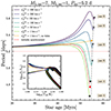Fig. 5.

Evolution of the orbital period of HD 25631 for different values of the initial rotational velocity (including initially synchronized rotation for a given P_ini). The tracks stop at the onset of Roche lobe overflow of the primary star. When this occurs during its main-sequence (case A) we mark it by dots, conversely, if this happens after TAMS (gray dashed line) in a case B, we mark it with crosses. For reference, the inset shows the HR diagram around TAMS, where the beginning of the RLOF phases are marked by thick black outlines. The red horizontal line visualizes the initial value of the orbital period. In these simulations we used the sync_type = “Hut_rad” tidal prescription.

Our simulations lead us to the conclusion that the spin-down timescale is comparable to the entire main-sequence lifetime of each star. For example, for 7 M_⊙ and 15 M_⊙ primaries (HD 25631 and HD 191495, respectively), the v_rot only drops by 4% and 6% from the initial value at the half of the main-sequence duration. In the case of the more massive (24 M_⊙) star HD 46485, the drop in v_rot is happening quicker (by 22% at half of main-sequence duration, assuming “Dutch” mass loss regime) because of the stronger mass loss rate for stars of larger initial mass. In addition to this, we show that tidal synchronization can spin up the star only at the end of the main-sequence when the size of the star is significantly larger than at ZAMS. In view of the young age of all studied systems (< 10 Myr, see Table 1 and Nazé et al. 2023) and our demonstration that the initial rotation can remain for a significant duration of the main-sequence (cf. Fig. 2), we suggest that the observed fast rotation of these systems can be primordial. With the current short orbital periods and extreme mass ratios, tidal synchronization only plays an important role during the latest stages of the main-sequence. This is in agreement with other studies of synchronization timescale of Algol systems that appeared to be longer and weaker than accretor’s spinning-up timescale due to mass transfer (see, e.g. Deschamps et al. 2013).

3.4. Future of the systems

We evolved the models presented in Sect. 3.2 until the onset of binary mass-transfer, occurring right at the end of the main-sequence or just after, depending on the initial rotation. Taking into account the rather extreme mass-ratios of these systems, it is natural to consider the common envelope (CE) scenario when investigating the future of our systems (Paczynski 1976; Claeys et al. 2014; Renzo et al. 2021).

The largest mass ratio q ≲ 0.15 (see Table 1) is indeed much smaller than the typical minimum threshold for stability (e.g., q ≥ q_crit ≃ 0.25 − 0.625 for main-sequence interactions, Claeys et al. 2014). Thus, we assume that the mass-transfer event will become dynamically unstable and result in a common envelope (CE) event (Paczynski 1976; Ivanova et al. 2013, 2020; Renzo et al. 2021).

We calculate the α_CE parameter (Webbink 1984) to discuss the chance of a successful ejection. This parameter measures the efficiency of the CE process in using orbital energy to lift the shared envelope,

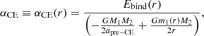
$\begin{matrix} α_{CE} \equiv α_{CE} (r) = \frac{E_{bind} (r)}{(- \frac{G M_{1} M_{2}}{2 a_{pre - CE}} + \frac{G m_{1} (r) M_{2}}{2 r})}, \end{matrix}$ $\begin{aligned} \alpha _{\rm CE} \equiv \alpha _{\rm CE}(r) = \frac{E_{\rm bind}(r)}{\left(-\frac{GM_1M_2}{2a_{\rm pre-CE}}+ \frac{Gm_1(r) M_2}{2r}\right)}, \end{aligned}$ (1)

where E_bind(r) is the binding energy profile (assumed to be “frozen” during the CE, thus we neglect the thermal and dynamical response of the envelope to the inspiral), G the gravitational constant, m₁ ≡ m₁(r) is the donor mass remaining inside r such that m₁(r = R₁) = M₁, M₂ is the companion mass, a_{pre − CE} is the binary separation at the moment of TAMS⁴ (i.e., ∼45.0 R_⊙, ∼25.7 R_⊙, ∼26.3 R_⊙ for HD 46485, HD 191495, and HD 25631 respectively). Formally, conservation of energy requires α_CE < 1 (Iaconi & De Marco 2019) although larger values are routinely considered to mimic the inclusion of energy sources other than the orbit in the common-envelope ejection process (Han et al. 1995; Ivanova et al. 2002; De Marco et al. 2011; Zorotovic et al. 2014).

To determine E_bind(r), we integrate the internal structure of our stellar models from the surface inward (e.g., Han et al. 1995; Dewi & Tauris 2000; Renzo et al. 2023):

$\begin{matrix} E_{bind} (m_{1} (r)) = - \int_{m_{1}}^{M_{1}} d m' (- \frac{G m'}{r (m')} + α_{th} u (m^{'})), \end{matrix}$ $\begin{aligned} E_{\rm bind}(m_1(r)) = - \int _{m_1}^{M_1}\,\mathrm{d}m^\prime \left(-\frac{G m\prime }{r(m\prime )}+\alpha _{\rm th}u(m\prime )\right), \end{aligned}$ (2)

where α_th is a tunable parameter to include (α_th = 1) or exclude (α_th = 0) the contribution of the internal energy u. Higher α_th result in a lower value of α_CE which then result in an ejection of the envelope down to a given depth r, corresponding to an optimistic ejection case (see, e.g., Klencki et al. 2021). Since our models predict the interaction to be very close to the end of the MS, we focus on the results derived at the latest steps of our simulations near the TAMS. This neglects the impact of the initial RLOF phase preceding the CE on the stellar structure and binding energy (e.g., Ivanova et al. 2020; Renzo et al. 2021; Blagorodnova et al. 2021). However, this impacts mostly the outer layers of the star and we expect it to be insufficient to change our conclusions.

Figure 6 presents the calculated α_CE for primaries of our three systems as a function of radius inside the star and for different tidal prescriptions including and excluding the internal energy contribution. It also shows the hydrogen mass fraction profile (X(¹H)) which decreases at the core-envelope boundary, see inset panel.

Fig. 6.

Efficiency of the CE process α_CE, with a different fraction of thermal energy α_th for our three targets (see text for details). In order to define the zone of the stellar core we indicated the mass fraction of X(¹H) by the gray line, linked to the right y-axis.

If, as we expect, the future mass transfer in the primordial scenario does result in a common envelope, α_CE needs to be lower than one for the companion to remove the entire envelope down to the hydrogen-depleted layers using only the orbital energy. Our simulations (Fig. 6) indicate results of α_CE estimates to be 3−6 for HD 25631, 5−13 for HD 191495, and 9−15 HD 46485. This strongly suggests that the envelope will not be successfully ejected, hence the systems will most probably merge in the future.

4. Spin-up – post-interaction scenario

Binaries can also produce fast-rotating stars during mass-transfer episodes. As the donor overfills its Roche lobe, the transferred mass carries angular momentum and, if successfully accreted by the companion star, deposits the angular momentum at its surface. The accretor gains a significant angular momentum and spin is increasing very quickly up to the critical rotation (Packet 1981; Langer et al. 2003; Renzo & Götberg 2021).

In this scenario, the observed star in the SB1 binaries under consideration has previously been spun up by accretion and the unseen companion is the stripped donor (e.g., Götberg et al. 2023; Drout et al. 2023) or its remnant. Given the difficulty of identifying stripped star companions, we still consider the binary mass transfer scenario to illustrate its impact on the orbital architecture, which would have made us disfavor this scenario even in absence of a detectable reflection effect. Thus, despite the fact that all three investigated systems are pre-interacting we still aim to model them within the post-interacting paradigm which could be useful for future studies. However, for this scenario to be valid for our targets, it needs to reproduce all parameters of the systems (mass-ratio, periods, age, etc.), not only fast rotation of the mass gainer.

4.1. Method

We use the binary module in MESA to evolve both stars in each binary system. To test whether post-interaction binary scenario is applicable to our systems, we built a grid of binaries with various masses of donor star (M_don = [30, 20, 10] M_⊙) and accretor’s masses (M_acc = [20, 15, 10, 7] M_⊙) that give mass ratios of Q = M_acc/M_don = [0.75, 0.7, 0.65, 0.5, 0.33]. For these systems we use initial periods of P_ini = [1.25, 3, 5, 10, 50, 70] days. Given the small observed eccentricity (Table 1), and the significant circularization timescale (Appendix D), we assume our binaries to be initially circular (e = 0). Our setup is closely based on Renzo & Götberg (2021), Renzo et al. (2023), and we summarize here the main physical and numerical choices regarding initial rotation and mass transfer. We refer to Appendix A and the previous section for further information.

We model Roche lobe overflow (RLOF) allowing for optically thick outflows (Kolb & Ritter 1990). Mass transfer is conservative up to the point when the accretor reaches the critical rotation $ω_{crit} = \sqrt{(1 - L / L_{Edd}) G M / R^{3}}$ $\omega_{\mathrm{crit}}=\sqrt{(1-L/L_{\mathrm{Edd}})GM/R^3}$ where centrifugal force plus radiation pressure equal gravity at the equator, with L_Edd the Eddington luminosity, and L the stellar luminosity (e.g., Petrovic et al. 2005; van den Heuvel et al. 2017). The transferred material carries the same specific angular momentum as the accretor surface, producing a relatively slow spin-up (Renzo & Götberg 2021). When the accretor’s surface approaches critical rotation, ω = 0.95 ω_crit, we enhance the accretor’s mass loss rate following Langer (1998), which briefly stops the accretion. The mass loss spins down the stars, resulting in accretion resuming in a “self-regulated” way, moderated by the inward angular momentum transport (e.g., Renzo & Götberg 2021). Overall, this leads to a mass transfer efficiency (η = ΔM_acc/ΔM_don as it has been introduced in Soberman et al. 1997) that actually varies depending on the orbital configuration i.e., in close binaries the mass transfer is more efficient (see the next subsection).

To test a lower limit on how fast the accretors may be spun up we initially assume rigid rotation with $v_{rot}^{ini} = 1$ $v_{\mathrm{rot}}^{\mathrm{ini}} = 1$ km s⁻¹ at the equator for both stars, regardless of the orbital period. Our models include tides, following the two prescriptions discussed in Sect. 3.2 – thus on a tidal timescale we expect the orbits to shrink slightly to spin up both stars.

4.2. Results and interpretation

As an illustrative example, we first focus on M_don, ini = 30 M_⊙ and M_acc, ini = 20 M_⊙, corresponding to Q = 0.65, close to the average value of a flat mass ratio distribution between 0.1 and 1, as observed in massive OB-type binaries (see Vanbeveren 1981; Sana et al. 2013). Moreover, to test the viability of the accretor scenario, we aim to reproduce with an accretor star the highest mass case among our fast rotators (HD 46485, M_1, obs = 24 M_⊙). As mentioned before, we did explore a larger range of parameters but it is important to note that all simulations lead us to similar conclusions, hence our choice to present in detail only one case.

Figure 7 illustrates the evolution of orbital period as a function of mass ratio for six cases of initial period by taking into account MESA default and POSYDON structure-dependent tide prescriptions (see Sect. 3.2). In these models, we wanted to reproduce the post-RLOF phase that would give the observed period, masses, and mass ratio. With initial periods above 10 days, the orbital periods increase as a result of mass transfer (e.g., Renzo et al. 2019), thus the systems do not match the observed range of periods. However, varying assumptions on the mass transfer efficiency and the angular momentum losses, this general trend can change. A natural way to prevent the orbital widening, is to assume mass transfer to be nonconservative and remove significant amount of angular momentum, for example because of the non-accreted material forms a circumbinary disk (CBD) which applies torques to the inner binary (see e.g., Vanbeveren 1982; Shao & Li 2016).

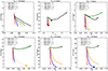Fig. 7.

Orbital period vs. mass ratio relation for six cases of initial orbital periods (1.25, 3, 5, 10, 50, and 70 days) and masses M_don, ini = 30 M_⊙ and M_acc, ini = 20 M_⊙. Different tidal synchronization prescription regimes i.e. sync_type = “Hut_rad” (MESA default) and sync_type = “structure_dependent” (POSYDON) are presented. In addition, different fractions of mass lost from circumbinary toroid (via changing the mass transfer efficiency parameters δ and γ, see text for details) are shown. The cases with γ = 0 refer to the conservative mass transfer scenario. The RLOF phases are marked by a bold line. Filled and open circles indicate the reasons of track termination: both stars filled their Roche lobes or numerical convergence problem, respectively. In the case of 1.25 day configuration, both stars filled their RL almost simultaneously and we consider that all tracks indicate a subsequent merging.

To test this scenario, we explore different mass transfer efficiencies, using the parametrized analytic formalism of Soberman et al. (1997). Namely, the mass transfer efficiency is defined as the ratio of the accretor’s mass change to the donor’s mass change at each timestep, i.e. η = ΔM_acc/ΔM_don. If the mass transfer is nonconservative (η ≠ 1), the fraction of mass that is lost to a (coplanar, unmodeled) CBD is defined as δ = 1 − η. Thus, in our simulations, we are continuously updating δ, by assuming three different sizes of the CBD. Namely, we vary the radius of CBD defined as r_CBD = γ²a, where γ = 1, 2, 10 is another free parameter. We assume no mass is lost in the vicinity of the accretor and donor (α and β equal to zero according to Soberman et al. 1997 formalism).

We illustrate how the modeled mass transfer efficiency varies as a function of average angular surface velocity in the Fig. 8 by assuming γ = 3 (see the resolution test in Fig. B.4). As we can see for the short-period models (P_ini = 3, 5 days), η is significantly larger than for the longer period configurations (as it has been also shown by Sen et al. 2022), which means that mass transfer is not efficient in a such regime of CBD for longer period systems. It can be explained: with larger orbital angular momentum (longer periods), more material from the donor remains in the CBD, thus the efficiency of accretion becomes low (as can be seen in Fig. 8). Notably, in such a regime of the nonconservative mass transfer, the accretor never reaches the 0.95 ω_crit threshold – because for P < 5 days all massive binaries with Q ∼ 0.65 reach tidal synchronization early in the MS. This analysis shows how sensitive is the mass transfer efficiency even in such a simple model of CBD existence. In addition, we tested binary models with the Fuller et al. (2019) AM transport and found this to have a negligible impact on η and on the accretor’s total angular momentum. Preliminary analysis shows that with a more efficient AM transport, it takes longer to spin up the accretor with respect to the less efficient AM transport (e.g. considering the Spruit – Tayler dynamo). To trace the exact history of the mass transfer and occurrence of the CBD we need to explore more complex models of mass transfer which is beyond the scope of the present work.

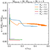Fig. 8.

Mass transfer efficiency (η) as a function of the surface average angular velocity for the various initial periods of a given system.

The behavior of P vs. Q tracks depends on the different assumed values of γ and this is presented in Fig. 7. As we can see, for initial periods near the current values (∼5 days), the orbital period either increases or decreases, depending on which mass transfer regime we are adopting. However, the value of Q always remains below 2, i.e., it does not come close to the extreme values that are observed in our systems: as we consider the post-interaction paradigm, the modeled Q should be the inverse of the observed (q) i.e. our systems should have Q > 5.

For shorter initial periods, the period further decreases, taking us away from the observed values. Moreover, in the majority of cases, the systems merge with the most extreme case (P_ini = 1.25 days) within 500−800 years following the onset of RLOF (see the first top panel of Fig. 7). Thus, during and after the donor’s RLOF stage, we can not reproduce the observed periods and mass ratios whatever the value of P_ini. Further simulations show, that in the majority of cases, the systems with periods less than 10 days will also merge. We identified the time of merging events as the time at which both the secondaries and the primaries fill their Roche Lobe and we indicated this by filled circles at the end of each track in Fig. 7.

In the case of larger initial periods (P_ini > 10 days, three bottom panels in Fig. 7), nonconservative mass transfer can form short-period systems, however, extreme mass ratios would be again difficult to reach. To confirm these results, we compute an additional set of models with different initial masses of the components. The results of these simulations confirm the main increasing trend of the mass ratio up to the possible merging of the systems (in a nonconservative mass transfer regime, in terms of η > 0) or up to the moment of system detachment (at conservative mass transfer regime, when η = 0). However, the value reached remain far from the observed ones. We can therefore conclude that the presented scenario to form short-period, extreme mass ratio, fast-rotating binaries from binary interaction is not favored.

Short-period binaries could form through a post CE scenario (see channel 4 in Willems & Kolb 2004). However, if we assume a post-CE origin of our systems, the rotational velocity of the current primary component will be conditioned only by tidal synchronization. As demonstrated in Sect. 3, it is not possible to reach the observed vsin i (exceeding tidal synchronization values), especially in the case of HD 46485. A post-common envelope ejection origin of our targets thus appears to be unlikely.

5. Merger in a triple

The majority of massive OB-type stars are born in high-multiplicity systems, with ∼60% having at least two companions, i.e. being in triple systems (e.g., Moe & Di Stefano 2017; Offner et al. 2023). Thus, we also consider a triple-evolution scenario to explain the rotation of the observed star in these systems. As we demonstrate below, the present day observed mass ratios of HD 25631, HD 191495, and HD 46485 imply that if they had a past as triple stars, they were hierarchical, m₁ + m₂ ≫ m₃, where m_i are the individual stellar masses (contrary to the previous sections where lower case m was used for mass-coordinate inside the star).

In this scenario, the current primary star in the observed system is the remnant of the merger of the inner binary in an originally triple system. The observed fast rotation comes from the (fraction of) orbital angular momentum of the inner binary retained by the merger product (e.g., de Mink et al. 2014). The observed present-day binary orbit corresponds to the initial outer binary orbit, possibly modified by the mass and angular momentum losses during the merger itself. Here, we discuss the reasons why we consider this scenario unlikely for HD 25631, HD 191495, and HD 46485, although it is hard to completely rule it out given the vast ten-dimensional parameter space for initial triple configurations (e.g., Toonen et al. 2016).

The mergers and fast rotation. Some multidimensional magneto-hydrodynamics simulations of mergers between main-sequence stars of masses comparable to ours (∼9 + 8 M_⊙) predicted the remnant to be slow rotating and magnetic (Schneider et al. 2016, 2019, 2020, see also Wang et al. 2020). The reason for the slow post-merger rotation is three-fold: (i) dynamical mass and angular-momentum loss during the merger itself, (ii) magnetic-braking post-merger, and most importantly, (iii) the internal readjustment of the merger product. In fact, the merger happens on a dynamical timescale, therefore the core structure of the initially more massive star is “frozen” during the process. The core settles in the center of the merger product, but initially retains its pre-merger density, set by the structure of a lower mass star. Post-merger, the structure has to readjust to the new and increased total mass by lowering its central density. Thus, on a thermal timescale, the core expands consuming angular momentum (Schneider et al. 2019, 2020).

In addition, the empirical initial rotation distributions for apparently single stars (Ramírez-Agudelo et al. 2013) and confirmed binaries (Ramírez-Agudelo et al. 2015) in 30 Doradus suggest that the fastest rotators detected are binary accretors (e.g., Packet 1981; Blaauw 1993; Renzo & Götberg 2021) and possibly mergers (e.g., de Mink et al. 2013). In fact, theoretical predictions for the surface and internal rotation of merger products can vary significantly as a function of mass ratio and evolutionary stage of the pre-merger binary (Chatzopoulos et al. 2020; Renzo et al. 2020). The angular momentum transport before, during, and after the merger is also highly uncertain (e.g., see discussion in Spruit 1999, 2002; Fuller et al. 2019; den Hartogh et al. 2020). For example, Chatzopoulos et al. (2020) proposed that Betelgeuse’s fast rotation (for a red-supergiant) may be explained with a post-MS merger. Because of these uncertainties, we do not consider the theoretical expectation of slow rotating merger products sufficient to discard a merger-in-a-triple scenario on its own.

Dynamical instability of putative triple progenitor. The present-day observed periods, corresponding to orbital separations of ∼24.6 R_⊙, 24.7 R_⊙, and 45 R_⊙, for HD 25631, HD 191495, and HD 46485, respectively, put strong constraints on the initial conditions for a triple. We treat the orbital evolution during the merger by analogy with the “Blaauw kick”, typically considered in the context of spherically symmetric⁵ supernova explosions in a binary (Blaauw 1961; Boersma 1961). The merger ejects a fraction f_Δ of the total mass of the inner binary. Hydrodynamical simulations of stellar collisions, such as the ones that may occur in an unstable triple system, usually produce f_Δ ≲ 12% (e.g., Lombardi et al. 2002; Glebbeek et al. 2013; Renzo et al. 2020; Ballone et al. 2023), so we explore two values of f_Δ = 0 and 0.1. We assume the ejecta leave the (triple) system instantaneously without interacting with the outer companion. Section 5 discusses further these approximations.

Throughout this section, we neglect the orbital widening caused by wind mass loss. In fact, the most massive star considered here is ∼24 M_⊙ and has an apparent age of ∼2 Myr. Theoretically, a solar-metallicity star of comparable mass loses ≲4 − 8% of its total mass over the entire main-sequence lasting ∼7 Myr (Renzo et al. 2017). Thus, we can assume that the present-day observed primary mass M₁ is the post-merger mass within a few percent precision. Correcting for the fraction of mass lost at merger f_Δ, gives the pre-merger total mass of the inner binary:

$\begin{matrix} M_{1} = m_{1} + m_{2} - f_{Δ} (m_{1} + m_{2}) \Rightarrow m_{1} + m_{2} = \frac{M_{1}}{1 - f_{Δ}}, \end{matrix}$ $\begin{aligned} M_1 = m_1+m_2 - f_\Delta (m_1+m_2) \Rightarrow m_1+m_2 = \frac{M_1}{1-f_\Delta }, \end{aligned}$ (3)

and since by construction m₁ and m₂ are individually smaller than M₁, we can again neglect wind mass loss rates pre-merger and consider m₁ + m₂ the total ZAMS mass of the inner binary. Similarly, neglecting wind mass loss, at ZAMS the tertiary star has a very similar mass as the present day secondary mass m₃ = M₂. Thus the outer binary mass ratio is known q_out = m₃/(m₁ + m₂) = M₂(1 − f_Δ)/M₁.

We can then find the range of initial inner separations a_in possible as a function of the unknown eccentricity e_in and mass ratio q_in of the inner binary, shown in Fig. 9. We define a lower boundary min(a_in) corresponding to inner binaries where both stars are filling their Roche lobe at periastron at ZAMS. To calculate the Roche lobe size at ZAMS, we use the Eggleton (1983) fitting formula R_RL, i = aE(q_i)≡R_RL, i(q_i) where a is the binary separation E(q_i) is an analytic function of the mass ratio q₁ = m₁/m₂ and q₂ = m₂/m₁. Although the Roche geometry is valid only in the restricted circular two-body problem, we approximately account for the eccentricity of the inner binary by approximating the elliptical orbit with a circular orbit with radius equal to the periastron, substituting a_in → a_in(1 − e_in). Thus, for each (q_in, e_in) pair we can impose the condition R_ZAMS, i ≤ R_RL, i ≡ R_RL, i(q_in, e_in) and translate it into a ≥ min(a_in)≡min(a_in)(q_in, e_in). For simplicity, we estimate the initial radii R_ZAMS, i using an analytic mass–radius relation for homogeneous polytropic stars, R_ZAMS, i = R_⊙(m_i/M_⊙)^ξ with ξ = 0.9 for M_i < 1.4 M_⊙ and ξ = 0.6 otherwise. Note that introducing a constraint depending on the ZAMS radii introduces a mass-dependence that breaks the scale-free nature of the Newtonian three-body problem.

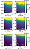Fig. 9.

Minimum initial inner binary separation min(a_in) to prevent RLOF at periastron at ZAMS (i.e., R₁(m₁)≤R_RL, 1 and R₂(m₂)≤R_RL, 2) as a function of the inner binary mass ratio q_in = m₂/m₁ and eccentricity e_in for HD 45485 (top), HD 191495 (middle), and HD 25631 (bottom). The red solid lines mark the present-day observed separation, corresponding to the evolved post-merger a_out in the merger-in-a-triple scenario, while the black area in the bottom left corners corresponds the unphysical region with initial inner binary separation with R_i(m_i)≤R_RL, i. In the bottom row, the boundary of this unphysical region has a kink caused by the change of slope in the assumed mass–radius relation: HD 25631 primary mass is M₁ ≃ 7 M_⊙, so for q_in ≲ 0.2 (the exact threshold depends on f_Δ), the expected values of m₂ are sufficiently low that the exponent ξ in the R_ZAMS ≡ R_ZAMS(m) changes. For the right column with f_Δ ≠ 0, our assumptions based on the Blaauw (1961) approximation may be inconsistent (see Sect. 5).

With the assumption of instantaneous mass loss from the inner binary (Blaauw 1961), the outer binary is either unperturbed (f_Δ = 0) or it widens and increases its eccentricity (f_Δ > 0). Thus, we expect the outer binary to have an initial separation shorter than that of the binaries observed today:

$\begin{matrix} a_{obs} ≳ a_{out, post - merger} ≳ a_{out, pre - merger} ≃ a_{out, ZAMS} \end{matrix}$ $\begin{aligned} a_{\rm obs} \gtrsim a_{\rm out,post-merger}\gtrsim a_{\rm out, pre-merger}\simeq a_{\rm out, ZAMS}\, \end{aligned}$ (4)

where we use the results of Sect. 3 to assume the binary is presently widening, once-again, we neglect widening caused by wind mass loss and secular orbital effects, and by definition a_out, ZAMS ≳ a_in, ZAMS ≳ min(a_in) (see Fig. 9). The Blaauw (1961) model assumes circular pre-mass-ejection binaries. Given the small observed eccentricities and the relative inefficiency of tides discussed in Sect. 3, we consider here pre-merger outer eccentricity equal to today’s observed value e_out = e_obs ≃ 0, which is consistent with f_Δ = 0 but in possible tension with nonzero mass loss mergers f_Δ ≠ 0 (see Sect. 5).

The triple merger scenario is meaningfully different from a pure binary evolution model only if the triple is initially dynamically stable and gets destabilized by stellar evolution processes (e.g., radial expansion, mass loss, tides, Perets & Kratter 2012). If that is not the case, the triple will either evolve chaotically (leading to a merger or disruption within a few Lyapunov times) or is unstable (leading to merger or disruption within a few dynamical times set by the inner/outer orbital period). Either of these scenarios would result in the prompt formation of a binary (compared to stellar evolution timescales) and reduce to the pre-interaction scenario discussed in Sect. 3. Conversely if a stable triple can form, the mass hierarchy implied by the present-day binaries suggests m₁ + m₂ ≫ m₃ for most measurable values of q_in = m₂/m₁. Therefore, in the original inner binary stellar evolution proceeds much faster, and instabilities in the triple triggered by the stellar evolution in the inner binary are likely (Perets & Kratter 2012), so we can limit our discussion to initially stable and non-chaotic triples.

With the physical constraints discussed above, we can build triple systems compatible with the observed binaries and quantify their dynamical stability. To explore the parameter space for triple systems, we draw 10⁶ initial triples for each observed binary and evaluate their dynamical stability⁶. We sample a uniform distributions in the range 0 ≤ e_in < 1 for the inner eccentricity, 0.1 ≤ q_in ≤ 1 for the inner binary mass ratio, min(a_in)≤a_in ≤ a_out ≤ a_obs for the inner and outer separations where a_obs is the present-day observed binary separation, 0 ≤ i_rel ≤ π for the mutual inclination of the inner and outer orbit, and 0 ≤ e_out ≤ e_obs for the outer eccentricity. Certain choice of f_Δ, q_in, and e_in result in the unphysical condition min(a_in)≥max(a_out) = a_obs. This means that no triple can form with the assumed parameters within the constraints of the scenario: we discard these systems leaving us with ∼8 × 10⁵ triples for each f_Δ and each observed binary.

Recently, machine-learning techniques have been applied to the determination of the dynamical stability of a triple system (e.g., Lalande & Trani 2022; Vynatheya et al. 2022, 2023). Here, we use the publicly available “ghost orbit” method presented in Vynatheya et al. (2023), which for every triple defined by the set of parameters (q_in, q_out, a_in/a_out, e_in, e_out, i_rel) provides a probability for the system to be dynamically unstable and/or chaotic P as a function of the initial architecture of the triple.

The stability criterion is based on the divergence of orbits initially differing slightly in a_in in direct N-body simulations over a time corresponding to ∼100 outer-periods. We emphasize that this does not account for close stellar encounters resulting in mergers during a chaotic phase of evolution because the stars are modeled as point masses, therefore P is really a measure of the probability of the triple system to be dynamically disrupted within 100 periods of the outer binary. The underlying N-body simulation neglects the arguments of periastron parameters (in other words, the relative phase of the inner and outer binary), which is known to affect the stability, and do not include general relativistic effects (not relevant for stellar triples). The performance of the model is slightly worse on retrograde orbit, but nevertheless improves over the semi-analytic stability criterion from Mardling & Aarseth (1999) and Vynatheya et al. (2022).

Each row in Fig. 10 shows the complementary cumulative distribution of the sampled triples as a function of the probability of being unstable for each of the observed binaries. For each curve, the y-value represents the fraction of triple systems that have probability P of being unstable greater or equal than the abscissa value, marginalized over all parameters. Regardless of the observed binary considered, ≳95% of possible triple systems have a probability ≳90% of being dynamically unstable, meaning they would disrupt within ≲100 outer orbital periods. The longest period binary has 7 days ≃ P_obs ≳ P_{out, pre − merger} (cf. Eq. (4)), this means the timescale for disruption is ≲100 × P_obs ≲ 700 days ≃ 2 years. Since the initial time is rather arbitrarily chosen to be at ZAMS (which is not physically defined with such temporal precision), we argue that such short times make the “triple merger scenario” virtually indistinguishable from the “primordial rotation scenario”: the merger has to occur before dynamical disruption of the system, therefore so close to ZAMS that it can be considered as part of the star formation process. We note also that the probability P is loosely correlated with the number of outer orbits completed before disruption, and the high values shown in Fig. 10 suggest the vast majority of the triples would disrupt in much less than 100 outer orbits, shortening the time since ZAMS even further.

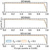Fig. 10.

Vast majority of triple systems compatible with the “merger in a triple” scenario has a probability of being dynamically unstable ≳90%. For each observed binary, we show the fraction of compatible putative triple progenitors that has a probability of being disrupted larger than the x coordinate according to the “ghost orbit” method of Vynatheya et al. (2023). Orange and blue curves correspond to the two values of fractional mass loss at merger f_Δ = 0 and 1 assumed. The distribution is marginalized over all parameters defining the architecture of the triples compatible with the present-day binaries (see text).

Nevertheless, the scenario is not completely ruled out, since a few percent of the simulated triple systems result in a very low probability of being unstable. Refining our understanding of the future evolution of survival initial triples, which depends on many initial parameters, would require an additional effort in numerical modeling (e.g. Toonen et al. 2020; Dorozsmai et al. 2024), which is beyond the scope of present work. Nevertheless, we note that most past triples are expected to be eccentric, which is not the case in our systems.

Caveats. Our arguments above require a few words of caution. The stability criterion we employ (see Vynatheya et al. 2023) ignores the occurrence of stellar mergers in the triple system, and is in this sense conservatively underestimating the probability of dynamical instability (a triple may be unstable because of mergers rather than disruption).

More importantly, if f_Δ ≠ 0, we have assumed that the merger ejecta leave the outer binary instantaneously and without interacting with the third companion. These assumptions result in an instantaneous widening and an increase in eccentricity of the outer binary. For the original application of Blaauw (1961) to supernova ejecta, this assumption is justified since ejecta velocity are ∼10⁴ km s⁻¹ ≫ v_orb where v_orb ≃ 10 − 100 km s⁻¹ is the orbital velocity of the binary containing the explosion. For our case of merger in a binary, with the constraints of the outer binary having a smaller orbital separation than today’s observed separation, this approximation is not as good and can even formally lead to absurd conclusion. We can estimate the ejecta velocity from the escape velocity of the inner binary $v_{ejecta} ≃ \sqrt{2 G (m_{1} + m_{2}) / a_{in}}$ $v_{\mathrm{ejecta}}\simeq \sqrt{2 G (m_1+m_2)/a_{\mathrm{in}}}$ and use Kepler’s third law to obtain the outer orbital velocity $v_{orb, out} = \sqrt{G (m_{1} + m_{2} + m_{3}) / a_{out}}$ $v_{\mathrm{orb, out}}=\sqrt{G(m_1+m_2+m_3)/a_{\mathrm{out}}}$ . The condition v_ejecta ≫ v_orb, out reduces to a_out/a_in ≫ 2(m₁ + m₂)/(m₁ + m₂ + m₃) which may not be possible to satisfy (depending on f_Δ). In most cases, our triple systems would have v_ejecta ≃ v_orb, out, which would require detailed (radiation)-hydrodynamical simulations of the interaction between the merger ejecta with the outer orbit to improve on the crude approximation of the Blaauw (1961) model. If the ejecta remain sufficiently dense as they cross a_out they may lead to a “triple common envelope” (e.g., Toonen et al. 2020) and a_out may shrink rather than expand because of the merger. Nevertheless, as discussed in the context of Fig. 4, post-common envelope tidal spin-up is not a valuable scenario for the mass ratio and ages observed.

6. Discussion

Based on our results described in the previous section, we conclude that primary stars in HD 25631, HD 191495, and HD 46485 are spinning faster than tidal synchronization most probably because of the results of star formation processes (pre-interaction scenario, Sect. 3) rather than binary interactions (Sect. 4) or a merger in a triple system (Sect. 5).

6.1. Observational context

We list in Table 2 all systems (including our targets) for which both photometric and spectroscopic analyses are available and the derived physical parameters are similar to our systems. Namely, we look for short-period OB-type massive binaries (P ≲ 10 days) with an extreme mass ratio (q ≲ 0.2), and fast rotation (vsin i ≳ 200 km s⁻¹).

Table 2.

Basic physical and orbital parameters for systems with a known fast-rotating OB star, extreme mass ratio, and short periods.

In the majority of cases, the resulting orbital solutions and spectroscopic disentangling suggest that identified O-type eclipsing binaries typically have pre-MS secondary components, which is in line with the detached pre-interaction phase being astrophysically long w.r.t. stellar lifetimes (i.e., HD 165246). Interestingly, according to Mahy et al. (2022), more long-period and highly eccentric binaries among the initial sample of SB1 fast rotators from Britavskiy et al. (2023) could possibly host a neutron star. However, according to their spectroscopic disentangling simulations, only the secondaries with M₂ ≳ 3 M_⊙ can be detected in the available spectra. Thus, there is a possibility that the secondary components are low-mass stars in pre-MS or MS stage (e.g., HD 15137 and HD 165174 in Mahy et al. 2022). That is in agreement with the P vs. q behavior shown in Fig. 7 for conservative mass transfer in Sect. 4: it is more likely to observe a post-interacting system in long period configurations.

Regarding B-type stars, in addition to the ones investigated in the present work, there are four other short-period binaries known with an extreme mass ratio, namely ν Cen, γ Lup A (see, Jerzykiewicz et al. 2021), HD 58730 (Stevens et al. 2020), and HD 149834 (Stassun et al. 2021). Companions in all these binaries are pre-MS stars, interestingly that HD 149834 and γ Lup A, harbour fast-rotating B-type stars (vsin i = 216 ± 11 km s⁻¹, vsin i = 236 ± 5 km s⁻¹ respectively), while ν Cen is a slow rotator with a vsin i = 65 ± 6 km s⁻¹. Also, HD 58730 is just below our rotation limit i.e. vsin i = 183 ± 1 km s⁻¹. In addition, about 20 short-period binaries with an extreme mass ratio have been detected in the Large Magellanic Cloud (see Moe & Di Stefano 2015). The lightcurves of these binaries are very similar to the objects we investigate in the present work, and Moe & Di Stefano (2015) suggest a pre-MS nature for the majority of the companions. Unfortunately, no spectroscopic analysis was performed so there is no information regarding the rotation rate of this sample of stars nor any radial velocity curves for these systems. In this context, there are also a couple of fast-rotating SB1 systems known in the Large Magellanic Cloud (O-type primaries, see Ramírez-Agudelo et al. 2015) and in the Small Magellanic Cloud (B-type primaries, see Bodensteiner et al. 2023). However, the orbital parameters of these binaries are yet unknown.

As we can see, all the stars from Table 2 with orbital periods P < 10 days have pre-MS or main-sequence companions in a pre-interacting stage. We can then draw the natural conclusion that the fast rotation of the primary OB star in each of the mentioned systems is primordial. Any binary interaction, including tides, would not result in high rotation velocity of the primary star in such short-period systems (see Sect. 3).

The formation of such rare binary configurations could be explained by protostellar disk fragmentation and further inward migration while accreting material at very early (< 0.1 Myr) evolutionary stages as was suggested by Tokovinin & Moe (2020). However, we do not have any observational constrain regarding the resulting distribution of stellar spin in this scenario. Such a distribution has only been studied for the pre-MS stars in the low-mass domain (see e.g., Serna et al. 2021; Kounkel et al. 2023), where longer lifetimes increase the importance of tides.

For the sake of completeness, we also checked the Multiple Star Catalog (Tokovinin 2018) in order to find any short period systems with a mass of primary components > 7 M_⊙ and q < 0.2. The result of this query consisted of 19 binary systems that are either detached binary systems or hierarchical triples or quadruples, none of these systems having stars with vsin i > 200 km s⁻¹. There are also short-period overcontact double-line spectroscopic binaries (see, e.g. Abdul-Masih et al. 2022), which in most cases appear to be tidally locked. These may appear as fast rotators as well (for example MY Cam and CC Cas, see Lorenzo et al. 2014; Southworth & Bowman 2022, respectively).

We should also mention a few known short-period post-interacting OB binaries. The systematized properties of selected well-studied post-interacting Be/Bn binaries can be found in Harmanec et al. (2015), Nazé et al. (2022), Schürmann et al. (2022), Wang et al. (2023b). Only a few systems with a period less than 10 days are known, and they are all rotating slower than our threshold: MX Pup (vsin i ∼ 120 km s⁻¹, P ∼ 5.15 days, Carrier et al. 2002), HD 15124 (vsin i ∼ 95 km s⁻¹, P ∼ 5.47 days, companion is a sdOB progenitor, El-Badry et al. 2022) and NGC 1850 BH1 (P ∼ 5.04 days, which leads to vsin i ∼ 50 − 70 km s⁻¹ by assuming the period of ellipsoidal variability and R ∼ 5 − 7 R_⊙, see El-Badry & Burdge 2022; Saracino et al. 2023). There also exist semi-detached B-type binaries with such short periods (see Table 7 in Harmanec et al. 2015) with an ongoing mass transfer. Nevertheless, none of the mentioned B-type systems has primaries rotating as fast as in the systems we focused on.

When considering longer period binaries, we note that there are more confirmed post-interacting companions in such short-period binaries with fast rotators of B-type than O-type. Partly, this is caused by the observational difficulties to detect a faint low-mass secondary component near a luminous massive O-type primary star. For example, the majority of sdOB objects were detected through UV spectroscopic observations (Wang et al. 2021), where the flux ratio of a hot stripped star with respect to the flux of a B-type star is more favorable than for O-type binary systems (Götberg et al. 2018).

In summary, known OB short-period binaries could either have a pre- or post-interacting companions, irrespective of the current rotation of their primaries, but extreme mass ratio and fast rotation seem to be found only in the pre-interacting systems. Thus, the fast-rotating tail observed for OB stars contains some fraction of pre-interacting objects, suggesting that physical processes active during the pre-MS may contribute to the high tail of the bimodal distribution of vsin i (Ramírez-Agudelo et al. 2015).

In favor of this hypothesis, we can also point out that the rotation distributions (up to vsin i ∼ 300 km s⁻¹) of apparently single O-type stars and of primaries in the spectroscopic binaries have the same morphologies (Ramírez-Agudelo et al. 2015). Considering our results on the fastest rotator in the sample (HD 46485), we can emphasize that even in the regime of highest rotation, the pre-interacting systems can be found. Thus, fast rotation alone is not sufficient to confidently advocate for a mass-transfer origin of fast rotators and other observables, such as chemical composition, apparent age, and kinematics (Blaauw 1961, 1993; Renzo et al. 2019; Renzo & Götberg 2021), should be considered to clean samples of binary accretors and reveal the initial rotation distribution of massive stars.

6.2. Theoretical implications

Our interpretation of HD 25631, HD 191495, and HD 46485 as short-period and extreme mass-ratio, massive binaries hosting a fast rotating primary since birth has several theoretical implications regarding star formation processes and early orbital evolution. As discussed above, rotation alone is not a sufficient smoking gun to establish the nature of an observed star as accretor, and a combination of signatures is desirable. These could include enhanced ¹⁴N and ⁴He at the surface (e.g., Blaauw 1993; Renzo & Götberg 2021), “rejuvenated” age (e.g., Neo et al. 1977; Schneider et al. 2016; Renzo et al. 2023), and possibly kinematic signatures (e.g., Renzo et al. 2019).

Also, our models suggest that formation processes can lead to primordial fast rotation, faster than initially tidally synchronized configuration where the orbital periods and rotational periods of both stars are equal, P_orb ≡ P_1, rot ≡ P_2, rot. Observations show instead P_1, rot < P_orb, which implies an excess angular momentum in the stellar spin, and thus makes tides widen the orbit in the initial phase of evolution (Sect. 3). Because the order of magnitude of spin angular momentum of a star (even at critical rotation) is much smaller than the orbital angular momentum, this is a relatively small effect, with typical orbital variations of Δa ≃ 12%⁷. This can cause a minor shift of boundary between case A and case B RLOF depending on the initial spin of the primary (see Fig. 5), potentially adding two extra dimensions (the initial rotation rate of both stars) to the parameter space for the evolution of binary systems. Moreover, this small increase in orbital separation a, although likely negligible, goes into the opposite direction compared to the “unspecified” orbital shrinking mechanism postulated to explain the early evolution of the radial velocity dispersion across young clusters (e.g., Sana et al. 2017; Ramírez-Tannus et al. 2021).

Tidal interactions in close binaries are a longstanding open question in stellar hydrodynamics. With the algorithms tested here (radiatively damped tides following Hut 1980 and layer-by-layer damping following Qin et al. 2018), and the low mass-ratios q ≲ 0.15 observed, tides are not able to significantly affect the spin of the primary star within the young inferred age. These algorithms have been compared before (e.g., Qin et al. 2018) and may not be representative of the full range of theoretical uncertainties (e.g., Ma & Fuller 2023; Sciarini et al. 2024), however, in both cases tides seem to be insufficient to significantly affect the observed rotation rate within the lifetime estimated for the primaries observed. One key uncertainty is that models of tidal synchronization are based on ZAMS models showing no core-envelope boundary: including the evolution of the stellar structure is expected to weaken the effect of tides further, strengthening our conclusions (Mirouh et al. 2023). Another factor to investigate how dynamical and equilibrium tides are affecting the synchronization and circularization timescales at different metallicity while the system is evolving (see, Siess et al. 2013).

7. Conclusions

In the present work, we evaluate different evolutionary scenarios that could explain the observed properties of three short-period binaries investigated by Nazé et al. (2023). Specifically, we consider three options for the origin of the faster than tidally synchronized rotation rate, spectroscopically observed in the SB1 systems HD 25631, HD 191495, and HD 46485: (i) star formation processes (the primordial and pre-interaction scenario), (ii) the result of spin-up due to mass transfer (post-interaction scenario), or (iii) the result of a merger in an originally triple system. The orbital architecture of the binaries (short observed period P < 10 days, small-to-null eccentricity e ≃ 0, and very low mass ratio q < 0.20) put strong constraints on the possible origin of the observed fast rotation.

Our analysis shows that:

Primordial fast rotation can persist during most of the MS stage, as the effect of the tidal interaction only starts to be significant close to the terminal age when the radius of the primary component is increasing.
Initial rotation affects the orbital configuration through the tidal interaction, widening the orbit in case of a large initial rotation thereby affecting when the mass transfer starts (before or after the MS stage, i.e., case A or case B mass transfer).
The evaluation of the post-interacting scenario leads us to the conclusion that during conservative mass transfer, the orbit widens significantly so this type of interaction cannot reproduce the present observational properties of the investigated systems (especially in terms of P and q).
Various regimes of nonconservative mass transfer can lead to short-period systems; however, it is unlikely to get an extreme mass ratio configuration before the systems merged as the orbit is shrinking fast.
An initially stable triple system may possibly result in a fast-rotating primary star after the merging of the inner binary. However, our current theoretical understanding suggests that MS mergers may be slow rotators and, most importantly, ∼95% of the simulated triple systems have a probability of being dynamically unstable ≳90%. This suggests that within ≲100 outer periods (≲2 years for our systems), the triple system would dynamically disrupt: this leaves an extremely narrow window for the merger to happen, and this would effectively reduce scenario (iii) to scenario (i) with the merger being part of the star formation process.

Thus, we suggest that it is likely that the primaries in our three systems have a fast-rotating primary from birth, that is, scenario (i) is preferred. These results support the protostellar disk fragmentation mechanism of forming short-period binaries suggested by Tokovinin & Moe (2020). The detection of such young pre-interacting binaries can shed light on the overall initial spin distribution of massive stars. In addition, if fast rotation can be primordial, it naturally implies that massive stars could have a wide range of initial rotations, and that rotation alone is not a sufficient indicator to uniquely identify past binary interactions.

¹

https://github.com/NikolayBritavskiyAstro/fast_rotating_binaries

²

https://zenodo.org/records/10479754

³

Resolution test for the model of the HD 46485 system is presented in Fig. B.2.

⁴

Among our systems only the HD 25631 reaches the TAMS before the mass transfer would start (case B), thus for the calculation of α_CE we used the required parameters at the moment of TAMS for HD 25631, and at the moment right before the mass transfer (case A) is started for the other systems.

⁵

Meaning no “natal kick” is imparted by asymmetries in the mass-shedding event, the explosion or, in our triple scenario, the merger.

⁶

The resulting triple populations with an estimate of their stability are publicly available at https://zenodo.org/records/10028333

⁷

Δa calculated as the maximum relative variation in orbital separation that we found among our systems (namely, in the case of HD 25631) at the moment the primary started the RLOF stage, when comparing the use of a $v_{rot}^{1, ini}$ $v_{\mathrm{rot}}^{\mathrm{1,ini}}$ = 1 km s⁻¹ to that of $v_{rot}^{1, ini}$ $v_{\mathrm{rot}}^{\mathrm{1,ini}}$ = 220 km s⁻¹.

Acknowledgments

We thank the anonymous referee for helpful comments that have improved the manuscript. The authors acknowledge M. Zapartas for the help with the tidal synchronization prescription that is implemented in the POSYDON code. N.B. acknowledges support from the postdoctoral program (IPD-STEMA) of Liege University, and the Belgian federal government grant for Ukrainian postdoctoral researchers (contract UF/2022/10). Y.N. and G.R. acknowledge support from the Fonds National de la Recherche Scientifique (Belgium), the European Space Agency (ESA), and the Belgian Federal Science Policy Office (BELSPO) in the framework of the PRODEX Programme (contract linked to XMM-Newton). M.R. thanks M. Cantiello and A. Trani for helpful discussion. Computational resources have been provided by the Consortium des Équipements de Calcul Intensif (CÉCI), funded by the Fonds de la Recherche Scientifique de Belgique (F.R.S.-FNRS) under Grant No. 2.5020.11 and by the Walloon Region.

References

Abbott, R., Abbott, T. D., Acernese, F., et al. 2023, Phys. Rev. X, 13, 041039 [Google Scholar]
Abdul-Masih, M., Escorza, A., Menon, A., Mahy, L., & Marchant, P. 2022, A&A, 666, A18 [NASA ADS] [CrossRef] [EDP Sciences] [Google Scholar]
Abt, H. A., & Moyd, K. I. 1973, ApJ, 182, 809 [NASA ADS] [CrossRef] [Google Scholar]
Almeida, L. A., Sana, H., Taylor, W., et al. 2017, A&A, 598, A84 [NASA ADS] [CrossRef] [EDP Sciences] [Google Scholar]
Angulo, C., Arnould, M., Rayet, M., et al. 1999, Nucl. Phys. A, 656, 3 [Google Scholar]
Ballone, A., Costa, G., Mapelli, M., et al. 2023, MNRAS, 519, 5191 [NASA ADS] [CrossRef] [Google Scholar]
Bastian, N., Kamann, S., Amard, L., et al. 2020, MNRAS, 495, 1978 [NASA ADS] [CrossRef] [Google Scholar]
Bavera, S. S., Fragos, T., Qin, Y., et al. 2020, A&A, 635, A97 [NASA ADS] [CrossRef] [EDP Sciences] [Google Scholar]
Björklund, R., Sundqvist, J. O., Puls, J., & Najarro, F. 2021, A&A, 648, A36 [EDP Sciences] [Google Scholar]
Björklund, R., Sundqvist, J. O., Singh, S. M., Puls, J., & Najarro, F. 2023, A&A, 676, A109 [NASA ADS] [CrossRef] [EDP Sciences] [Google Scholar]
Blaauw, A. 1961, Bull. Astron. Inst. Neth., 15, 265 [NASA ADS] [Google Scholar]
Blaauw, A. 1993, in Massive Stars: Their Lives in the Interstellar Medium, eds. J. P. Cassinelli, & E. B. Churchwell, ASP Conf. Ser., 35, 207 [NASA ADS] [Google Scholar]
Blagorodnova, N., Klencki, J., Pejcha, O., et al. 2021, A&A, 653, A134 [NASA ADS] [CrossRef] [EDP Sciences] [Google Scholar]
Bodensteiner, J., Shenar, T., & Sana, H. 2020, A&A, 641, A42 [NASA ADS] [CrossRef] [EDP Sciences] [Google Scholar]
Bodensteiner, J., Sana, H., Dufton, P. L., et al. 2023, A&A, 680, A32 [NASA ADS] [CrossRef] [EDP Sciences] [Google Scholar]
Boersma, J. 1961, Bull. Astron. Inst. Neth., 15, 291 [NASA ADS] [Google Scholar]
Bragança, G. A., Daflon, S., Cunha, K., et al. 2012, AJ, 144, 130 [CrossRef] [Google Scholar]
Britavskiy, N., Simón-Díaz, S., Holgado, G., et al. 2023, A&A, 672, A22 [NASA ADS] [CrossRef] [EDP Sciences] [Google Scholar]
Brott, I., Evans, C. J., Hunter, I., et al. 2011, A&A, 530, A116 [NASA ADS] [CrossRef] [EDP Sciences] [Google Scholar]
Buchler, J. R., & Yueh, W. R. 1976, ApJ, 210, 440 [NASA ADS] [CrossRef] [Google Scholar]
Callister, T. A., Haster, C.-J., Ng, K. K. Y., Vitale, S., & Farr, W. M. 2021, ApJ, 922, L5 [NASA ADS] [CrossRef] [Google Scholar]
Carrier, F., Burki, G., & Burnet, M. 2002, A&A, 385, 488 [NASA ADS] [CrossRef] [EDP Sciences] [Google Scholar]
Cassisi, S., Potekhin, A. Y., Pietrinferni, A., Catelan, M., & Salaris, M. 2007, ApJ, 661, 1094 [NASA ADS] [CrossRef] [Google Scholar]
Cazorla, C., Nazé, Y., Morel, T., et al. 2017, A&A, 604, A123 [NASA ADS] [CrossRef] [EDP Sciences] [Google Scholar]
Chatzopoulos, E., Frank, J., Marcello, D. C., & Clayton, G. C. 2020, ApJ, 896, 50 [NASA ADS] [CrossRef] [Google Scholar]
Chugunov, A. I., Dewitt, H. E., & Yakovlev, D. G. 2007, Phys. Rev. D, 76, 025028 [NASA ADS] [CrossRef] [Google Scholar]
Claeys, J. S. W., Pols, O. R., Izzard, R. G., Vink, J., & Verbunt, F. W. M. 2014, A&A, 563, A83 [NASA ADS] [CrossRef] [EDP Sciences] [Google Scholar]
Claret, A., & Torres, G. 2018, ApJ, 859, 100 [Google Scholar]
Conti, P. S., & Ebbets, D. 1977, ApJ, 213, 438 [CrossRef] [Google Scholar]
Cyburt, R. H., Amthor, A. M., Ferguson, R., et al. 2010, ApJS, 189, 240 [NASA ADS] [CrossRef] [Google Scholar]
de Jager, C., Nieuwenhuijzen, H., & van der Hucht, K. A. 1988, A&AS, 72, 259 [NASA ADS] [Google Scholar]
De Marco, O., Passy, J.-C., Moe, M., et al. 2011, MNRAS, 411, 2277 [CrossRef] [Google Scholar]
de Mink, S. E., Langer, N., Izzard, R. G., Sana, H., & de Koter, A. 2013, ApJ, 764, 166 [Google Scholar]
de Mink, S. E., Sana, H., Langer, N., Izzard, R. G., & Schneider, F. R. N. 2014, ApJ, 782, 7 [Google Scholar]
den Hartogh, J. W., Eggenberger, P., & Deheuvels, S. 2020, A&A, 634, L16 [NASA ADS] [CrossRef] [EDP Sciences] [Google Scholar]
Deschamps, R., Siess, L., Davis, P. J., & Jorissen, A. 2013, A&A, 557, A40 [NASA ADS] [CrossRef] [EDP Sciences] [Google Scholar]
Dewi, J. D. M., & Tauris, T. M. 2000, A&A, 360, 1043 [NASA ADS] [Google Scholar]
Dodd, J. M., Oudmaijer, R. D., Radley, I. C., Vioque, M., & Frost, A. J. 2024, MNRAS, 527, 3076 [Google Scholar]
Dorozsmai, A., Toonen, S., Vigna-Gómez, A., de Mink, S. E., & Kummer, F. 2024, MNRAS, 527, 9782 [Google Scholar]
Drout, M. R., Götberg, Y., Ludwig, B. A., et al. 2023, Science, 382, 1287 [NASA ADS] [CrossRef] [Google Scholar]
Duchêne, G., & Kraus, A. 2013, ARA&A, 51, 269 [Google Scholar]
Dufton, P. L., Langer, N., Dunstall, P. R., et al. 2013, A&A, 550, A109 [NASA ADS] [CrossRef] [EDP Sciences] [Google Scholar]
Dunstall, P. R., Dufton, P. L., Sana, H., et al. 2015, A&A, 580, A93 [NASA ADS] [CrossRef] [EDP Sciences] [Google Scholar]
Eggleton, P. P. 1983, ApJ, 268, 368 [Google Scholar]
Ekström, S., Georgy, C., Eggenberger, P., et al. 2012, A&A, 537, A146 [Google Scholar]
El-Badry, K., & Burdge, K. B. 2022, MNRAS, 511, 24 [NASA ADS] [CrossRef] [Google Scholar]
El-Badry, K., & Quataert, E. 2021, MNRAS, 502, 3436 [NASA ADS] [CrossRef] [Google Scholar]
El-Badry, K., Conroy, C., Quataert, E., et al. 2022, MNRAS, 516, 3602 [NASA ADS] [CrossRef] [Google Scholar]
Ferguson, J. W., Alexander, D. R., Allard, F., et al. 2005, ApJ, 623, 585 [Google Scholar]
Fragos, T., Andrews, J. J., Bavera, S. S., et al. 2023, ApJS, 264, 45 [NASA ADS] [CrossRef] [Google Scholar]
Frémat, Y., Zorec, J., Hubert, A. M., & Floquet, M. 2005, A&A, 440, 305 [NASA ADS] [CrossRef] [EDP Sciences] [Google Scholar]
Fuller, J., & Lu, W. 2022, MNRAS, 511, 3951 [NASA ADS] [CrossRef] [Google Scholar]
Fuller, G. M., Fowler, W. A., & Newman, M. J. 1985, ApJ, 293, 1 [NASA ADS] [CrossRef] [Google Scholar]
Fuller, J., Piro, A. L., & Jermyn, A. S. 2019, MNRAS, 485, 3661 [NASA ADS] [Google Scholar]
Glebbeek, E., Gaburov, E., Portegies Zwart, S., & Pols, O. R. 2013, MNRAS, 434, 3497 [NASA ADS] [CrossRef] [Google Scholar]
Gormaz-Matamala, A. C., Cuadra, J., Meynet, G., & Curé, M. 2023, A&A, 673, A109 [NASA ADS] [CrossRef] [EDP Sciences] [Google Scholar]
Götberg, Y., de Mink, S. E., Groh, J. H., et al. 2018, A&A, 615, A78 [NASA ADS] [CrossRef] [EDP Sciences] [Google Scholar]
Götberg, Y., Drout, M. R., Ji, A. P., et al. 2023, ApJ, 959, 125 [CrossRef] [Google Scholar]
Han, Z., Podsiadlowski, P., & Eggleton, P. P. 1995, MNRAS, 272, 800 [NASA ADS] [Google Scholar]
Harmanec, P., Koubský, P., Nemravová, J. A., et al. 2015, A&A, 573, A107 [NASA ADS] [CrossRef] [EDP Sciences] [Google Scholar]
Heger, A., Langer, N., & Woosley, S. E. 2000, ApJ, 528, 368 [NASA ADS] [CrossRef] [Google Scholar]
Hendriks, D. D., & Izzard, R. G. 2023, MNRAS, 524, 4315 [NASA ADS] [CrossRef] [Google Scholar]
Herwig, F. 2000, A&A, 360, 952 [NASA ADS] [Google Scholar]
Holgado, G., Simón-Díaz, S., Herrero, A., & Barbá, R. H. 2022, A&A, 665, A150 [NASA ADS] [CrossRef] [EDP Sciences] [Google Scholar]
Huang, W., Gies, D. R., & McSwain, M. V. 2010, ApJ, 722, 605 [Google Scholar]
Hurley, J. R., Tout, C. A., & Pols, O. R. 2002, MNRAS, 329, 897 [Google Scholar]
Hut, P. 1980, A&A, 92, 167 [NASA ADS] [Google Scholar]
Hut, P. 1981, A&A, 99, 126 [NASA ADS] [Google Scholar]
Iaconi, R., & De Marco, O. 2019, MNRAS, 490, 2550 [Google Scholar]
Iglesias, C. A., & Rogers, F. J. 1993, ApJ, 412, 752 [Google Scholar]
Iglesias, C. A., & Rogers, F. J. 1996, ApJ, 464, 943 [NASA ADS] [CrossRef] [Google Scholar]
Itoh, N., Hayashi, H., Nishikawa, A., & Kohyama, Y. 1996, ApJS, 102, 411 [NASA ADS] [CrossRef] [Google Scholar]
Ivanova, N., Podsiadlowski, P., & Spruit, H. 2002, MNRAS, 334, 819 [NASA ADS] [CrossRef] [Google Scholar]
Ivanova, N., Justham, S., Chen, X., et al. 2013, A&ARv, 21, 59 [Google Scholar]
Ivanova, N., Justham, S., & Ricker, P. 2020, Common Envelope Evolution (Bristol: IOP Publishing) [Google Scholar]
Jermyn, A. S., Bauer, E. B., Schwab, J., et al. 2023, ApJS, 265, 15 [NASA ADS] [CrossRef] [Google Scholar]
Jerzykiewicz, M., Pigulski, A., Michalska, G., et al. 2021, MNRAS, 503, 5554 [Google Scholar]
Ji, S., Fuller, J., & Lecoanet, D. 2023, MNRAS, 521, 5372 [NASA ADS] [CrossRef] [Google Scholar]
Johnston, C. 2021, A&A, 655, A29 [NASA ADS] [CrossRef] [EDP Sciences] [Google Scholar]
Johnston, C., Aimar, N., Abdul-Masih, M., et al. 2021, MNRAS, 503, 1124 [NASA ADS] [CrossRef] [Google Scholar]
Kamann, S., Saracino, S., Bastian, N., et al. 2023, MNRAS, 518, 1505 [Google Scholar]
Kazeroni, R., Guilet, J., & Foglizzo, T. 2017, MNRAS, 471, 914 [NASA ADS] [CrossRef] [Google Scholar]
Keszthelyi, Z., Puls, J., & Wade, G. A. 2017, A&A, 598, A4 [NASA ADS] [CrossRef] [EDP Sciences] [Google Scholar]
Kippenhahn, R., & Weigert, A. 1967, Z. Astrophys., 65, 251 [NASA ADS] [Google Scholar]
Klencki, J., Nelemans, G., Istrate, A. G., & Chruslinska, M. 2021, A&A, 645, A54 [EDP Sciences] [Google Scholar]
Kobulnicky, H. A., Kiminki, D. C., Lundquist, M. J., et al. 2014, ApJS, 213, 34 [Google Scholar]
Kolb, U., & Ritter, H. 1990, A&A, 236, 385 [NASA ADS] [Google Scholar]
Kounkel, M., Stassun, K. G., Hillenbrand, L. A., et al. 2023, AJ, 165, 182 [NASA ADS] [CrossRef] [Google Scholar]
Lalande, F., & Trani, A. A. 2022, ApJ, 938, 18 [NASA ADS] [CrossRef] [Google Scholar]
Langanke, K., & Martínez-Pinedo, G. 2000, Nucl. Phys. A, 673, 481 [NASA ADS] [CrossRef] [Google Scholar]
Langer, N. 1998, A&A, 329, 551 [NASA ADS] [Google Scholar]
Langer, N. 2012, ARA&A, 50, 107 [CrossRef] [Google Scholar]
Langer, N., Yoon, S. C., Petrovic, J., & Heger, A. 2003, ArXiv e-prints [arXiv:astro-ph/0302232] [Google Scholar]
Ledoux, P. 1947, ApJ, 105, 305 [NASA ADS] [CrossRef] [Google Scholar]
Limongi, M., & Chieffi, A. 2018, ApJS, 237, 13 [NASA ADS] [CrossRef] [Google Scholar]
Lombardi, J. C., Jr., Warren, J. S., Rasio, F. A., Sills, A., & Warren, A. R. 2002, ApJ, 568, 939 [NASA ADS] [CrossRef] [Google Scholar]
Lorenzo, J., Negueruela, I., Baker, A. K. F. V., et al. 2014, A&A, 572, A110 [NASA ADS] [CrossRef] [EDP Sciences] [Google Scholar]
Ma, L., & Fuller, J. 2023, ApJ, 952, 53 [CrossRef] [Google Scholar]
MacFadyen, A. I., & Woosley, S. E. 1999, ApJ, 524, 262 [NASA ADS] [CrossRef] [Google Scholar]
Maeder, A., & Meynet, G. 2000, A&A, 361, 159 [NASA ADS] [Google Scholar]
Mahy, L., Sana, H., Shenar, T., et al. 2022, A&A, 664, A159 [NASA ADS] [CrossRef] [EDP Sciences] [Google Scholar]
Mardling, R., & Aarseth, S. 1999, in The Dynamics of Small Bodies in the Solar System, A Major Key to Solar System Studies, eds. B. A. Steves, & A. E. Roy, NATO Adv. Study Inst. (ASI) Ser. C, 522, 385 [NASA ADS] [CrossRef] [Google Scholar]
Mason, B. D., Hartkopf, W. I., Gies, D. R., Henry, T. J., & Helsel, J. W. 2009, AJ, 137, 3358 [Google Scholar]
Mirouh, G. M., Hendriks, D. D., Dykes, S., Moe, M., & Izzard, R. G. 2023, MNRAS, 524, 3978 [NASA ADS] [CrossRef] [Google Scholar]
Moe, M., & Di Stefano, R. 2015, ApJ, 801, 113 [NASA ADS] [CrossRef] [Google Scholar]
Moe, M., & Di Stefano, R. 2017, ApJS, 230, 15 [Google Scholar]
Mokiem, M. R., de Koter, A., Vink, J. S., et al. 2007, A&A, 473, 603 [NASA ADS] [CrossRef] [EDP Sciences] [Google Scholar]
Nazé, Y., Rauw, G., Smith, M. A., & Motch, C. 2022, MNRAS, 516, 3366 [CrossRef] [Google Scholar]
Nazé, Y., Britavskiy, N., Rauw, G., Labadie-Bartz, J., & Simón-Díaz, S. 2023, MNRAS, 525, 1641 [CrossRef] [Google Scholar]
Neo, S., Miyaji, S., Nomoto, K., & Sugimoto, D. 1977, PASJ, 29, 249 [NASA ADS] [Google Scholar]
Oda, T., Hino, M., Muto, K., Takahara, M., & Sato, K. 1994, At. Data Nucl. Data Tables, 56, 231 [NASA ADS] [CrossRef] [Google Scholar]
Offner, S. S. R., Moe, M., Kratter, K. M., et al. 2023, in Protostars and Planets VII, eds. S. Inutsuka, Y. Aikawa, T. Muto, K. Tomida, & M. Tamura, ASP Conf. Ser., 534, 275 [NASA ADS] [Google Scholar]
Packet, W. 1981, A&A, 102, 17 [NASA ADS] [Google Scholar]
Paczynski, B. 1976, in Structure and Evolution of Close Binary Systems, eds. P. Eggleton, S. Mitton, & J. Whelan, 73, 75 [NASA ADS] [CrossRef] [Google Scholar]
Pauli, D., Langer, N., Aguilera-Dena, D. R., Wang, C., & Marchant, P. 2022, A&A, 667, A58 [NASA ADS] [CrossRef] [EDP Sciences] [Google Scholar]
Paxton, B., Bildsten, L., Dotter, A., et al. 2011, ApJS, 192, 3 [Google Scholar]
Paxton, B., Cantiello, M., Arras, P., et al. 2013, ApJS, 208, 4 [Google Scholar]
Paxton, B., Marchant, P., Schwab, J., et al. 2015, ApJS, 220, 15 [Google Scholar]
Paxton, B., Schwab, J., Bauer, E. B., et al. 2018, ApJS, 234, 34 [NASA ADS] [CrossRef] [Google Scholar]
Paxton, B., Smolec, R., Schwab, J., et al. 2019, ApJS, 243, 10 [Google Scholar]
Penny, L. R., & Gies, D. R. 2009, ApJ, 700, 844 [Google Scholar]
Perets, H. B., & Kratter, K. M. 2012, ApJ, 760, 99 [NASA ADS] [CrossRef] [Google Scholar]
Petrovic, J., Langer, N., & van der Hucht, K. A. 2005, A&A, 435, 1013 [NASA ADS] [CrossRef] [EDP Sciences] [Google Scholar]
Pols, O. R., & Marinus, M. 1994, A&A, 288, 475 [NASA ADS] [Google Scholar]
Pols, O. R., Tout, C. A., Eggleton, P. P., & Han, Z. 1995, MNRAS, 274, 964 [Google Scholar]
Potekhin, A. Y., & Chabrier, G. 2010, Contrib. Plasma Phys., 50, 82 [NASA ADS] [CrossRef] [Google Scholar]
Preece, H. P., Hamers, A. S., Neunteufel, P. G., Schaefer, A. L., & Tout, C. A. 2022, ApJ, 933, 25 [NASA ADS] [CrossRef] [Google Scholar]
Qin, Y., Fragos, T., Meynet, G., et al. 2018, A&A, 616, A28 [NASA ADS] [CrossRef] [EDP Sciences] [Google Scholar]
Ramachandran, V., Hamann, W. R., Oskinova, L. M., et al. 2019, A&A, 625, A104 [NASA ADS] [CrossRef] [EDP Sciences] [Google Scholar]
Ramírez-Agudelo, O. H., Simón-Díaz, S., Sana, H., et al. 2013, A&A, 560, A29 [NASA ADS] [CrossRef] [EDP Sciences] [Google Scholar]
Ramírez-Agudelo, O. H., Sana, H., de Mink, S. E., et al. 2015, A&A, 580, A92 [NASA ADS] [CrossRef] [EDP Sciences] [Google Scholar]
Ramírez-Tannus, M. C., Backs, F., de Koter, A., et al. 2021, A&A, 645, L10 [NASA ADS] [CrossRef] [EDP Sciences] [Google Scholar]
Reig, P. 2011, Ap&SS, 332, 1 [Google Scholar]
Renzo, M., & Götberg, Y. 2021, ApJ, 923, 277 [NASA ADS] [CrossRef] [Google Scholar]
Renzo, M., Ott, C. D., Shore, S. N., & de Mink, S. E. 2017, A&A, 603, A118 [NASA ADS] [CrossRef] [EDP Sciences] [Google Scholar]
Renzo, M., Zapartas, E., de Mink, S. E., et al. 2019, A&A, 624, A66 [NASA ADS] [CrossRef] [EDP Sciences] [Google Scholar]
Renzo, M., Cantiello, M., Metzger, B. D., & Jiang, Y. F. 2020, ApJ, 904, L13 [NASA ADS] [CrossRef] [Google Scholar]
Renzo, M., Callister, T., Chatziioannou, K., et al. 2021, ApJ, 919, 128 [NASA ADS] [CrossRef] [Google Scholar]
Renzo, M., Zapartas, E., Justham, S., et al. 2023, ApJ, 942, L32 [NASA ADS] [CrossRef] [Google Scholar]
Rivinius, T., Carciofi, A. C., & Martayan, C. 2013, A&ARv, 21, 69 [Google Scholar]
Rogers, F. J., & Nayfonov, A. 2002, ApJ, 576, 1064 [Google Scholar]
Rosen, A. L., Krumholz, M. R., & Ramirez-Ruiz, E. 2012, ApJ, 748, 97 [NASA ADS] [CrossRef] [Google Scholar]
Sana, H., de Mink, S. E., de Koter, A., et al. 2012, Science, 337, 444 [Google Scholar]
Sana, H., de Koter, A., de Mink, S. E., et al. 2013, A&A, 550, A107 [NASA ADS] [CrossRef] [EDP Sciences] [Google Scholar]
Sana, H., Ramírez-Tannus, M. C., de Koter, A., et al. 2017, A&A, 599, L9 [NASA ADS] [CrossRef] [EDP Sciences] [Google Scholar]
Saracino, S., Shenar, T., Kamann, S., et al. 2023, MNRAS, 521, 3162 [NASA ADS] [CrossRef] [Google Scholar]
Saumon, D., Chabrier, G., & van Horn, H. M. 1995, ApJS, 99, 713 [NASA ADS] [CrossRef] [Google Scholar]
Schneider, F. R. N., Langer, N., de Koter, A., et al. 2014, A&A, 570, A66 [NASA ADS] [CrossRef] [EDP Sciences] [Google Scholar]
Schneider, F. R. N., Podsiadlowski, P., Langer, N., Castro, N., & Fossati, L. 2016, MNRAS, 457, 2355 [Google Scholar]
Schneider, F. R. N., Ohlmann, S. T., Podsiadlowski, P., et al. 2019, Nature, 574, 211 [Google Scholar]
Schneider, F. R. N., Ohlmann, S. T., Podsiadlowski, P., et al. 2020, MNRAS, 495, 2796 [NASA ADS] [CrossRef] [Google Scholar]
Schürmann, C., Langer, N., Xu, X., & Wang, C. 2022, A&A, 667, A122 [NASA ADS] [CrossRef] [EDP Sciences] [Google Scholar]
Sciarini, L., Ekström, S., Eggenberger, P., et al. 2024, A&A, 681, L1 [NASA ADS] [CrossRef] [EDP Sciences] [Google Scholar]
Sen, K., Langer, N., Marchant, P., et al. 2022, A&A, 659, A98 [NASA ADS] [CrossRef] [EDP Sciences] [Google Scholar]
Serna, J., Hernandez, J., Kounkel, M., et al. 2021, ApJ, 923, 177 [NASA ADS] [CrossRef] [Google Scholar]
Shao, Y., & Li, X.-D. 2016, ApJ, 833, 108 [NASA ADS] [CrossRef] [Google Scholar]
Siess, L., Izzard, R. G., Davis, P. J., & Deschamps, R. 2013, A&A, 550, A100 [NASA ADS] [CrossRef] [EDP Sciences] [Google Scholar]
Simón-Díaz, S., & Herrero, A. 2014, A&A, 562, A135 [NASA ADS] [CrossRef] [EDP Sciences] [Google Scholar]
Smith, N. 2014, ARA&A, 52, 487 [NASA ADS] [CrossRef] [Google Scholar]
Soberman, G. E., Phinney, E. S., & van den Heuvel, E. P. J. 1997, A&A, 327, 620 [NASA ADS] [Google Scholar]
Southworth, J., & Bowman, D. M. 2022, MNRAS, 513, 3191 [Google Scholar]
Spruit, H. C. 1999, A&A, 349, 189 [NASA ADS] [Google Scholar]
Spruit, H. C. 2002, A&A, 381, 923 [CrossRef] [EDP Sciences] [Google Scholar]
Stassun, K. G., Torres, G., Johnston, C., et al. 2021, ApJ, 910, 133 [NASA ADS] [CrossRef] [Google Scholar]
Stevens, D. J., Zhou, G., Johnson, M. C., et al. 2020, MNRAS, 499, 3775 [NASA ADS] [CrossRef] [Google Scholar]
Sweet, P. A. 1950, MNRAS, 110, 548 [Google Scholar]
Tayler, R. J. 1973, MNRAS, 165, 39 [NASA ADS] [Google Scholar]
Timmes, F. X., & Swesty, F. D. 2000, ApJS, 126, 501 [NASA ADS] [CrossRef] [Google Scholar]
Tokovinin, A. 2018, ApJS, 235, 6 [NASA ADS] [CrossRef] [Google Scholar]
Tokovinin, A., & Moe, M. 2020, MNRAS, 491, 5158 [NASA ADS] [CrossRef] [Google Scholar]
Toonen, S., Hamers, A., & Portegies Zwart, S. 2016, Comput. Astrophys. Cosmol., 3, 6 [NASA ADS] [CrossRef] [Google Scholar]
Toonen, S., Portegies Zwart, S., Hamers, A. S., & Bandopadhyay, D. 2020, A&A, 640, A16 [NASA ADS] [CrossRef] [EDP Sciences] [Google Scholar]
Vanbeveren, D. 1981, A&A, 95, 321 [NASA ADS] [Google Scholar]
Vanbeveren, D. 1982, A&A, 105, 260 [NASA ADS] [Google Scholar]
van den Heuvel, E. P. J., Portegies Zwart, S. F., & de Mink, S. E. 2017, MNRAS, 471, 4256 [Google Scholar]
Vinciguerra, S., Neijssel, C. J., Vigna-Gómez, A., et al. 2020, MNRAS, 498, 4705 [NASA ADS] [CrossRef] [Google Scholar]
Vink, J. S., de Koter, A., & Lamers, H. J. G. L. M. 2001, A&A, 369, 574 [NASA ADS] [CrossRef] [EDP Sciences] [Google Scholar]
Vynatheya, P., Hamers, A. S., Mardling, R. A., & Bellinger, E. P. 2022, MNRAS, 516, 4146 [NASA ADS] [CrossRef] [Google Scholar]
Vynatheya, P., Mardling, R. A., & Hamers, A. S. 2023, MNRAS, 525, 2388 [NASA ADS] [CrossRef] [Google Scholar]
Wang, L., Gies, D. R., & Peters, G. J. 2018, ApJ, 853, 156 [Google Scholar]
Wang, C., Langer, N., Schootemeijer, A., et al. 2020, ApJ, 888, L12 [NASA ADS] [CrossRef] [Google Scholar]
Wang, L., Gies, D. R., Peters, G. J., et al. 2021, AJ, 161, 248 [Google Scholar]
Wang, C., Hastings, B., Schootemeijer, A., et al. 2023a, A&A, 670, A43 [NASA ADS] [CrossRef] [EDP Sciences] [Google Scholar]
Wang, L., Gies, D. R., Peters, G. J., & Han, Z. 2023b, AJ, 165, 203 [NASA ADS] [CrossRef] [Google Scholar]
Webbink, R. F. 1984, ApJ, 277, 355 [NASA ADS] [CrossRef] [Google Scholar]
Willems, B., & Kolb, U. 2004, A&A, 419, 1057 [NASA ADS] [CrossRef] [EDP Sciences] [Google Scholar]
Wolff, S. C., Edwards, S., & Preston, G. W. 1982, ApJ, 252, 322 [NASA ADS] [CrossRef] [Google Scholar]
Wolff, S. C., Strom, S. E., Dror, D., & Venn, K. 2007, AJ, 133, 1092 [Google Scholar]
Xin, C., Renzo, M., & Metzger, B. D. 2022, MNRAS, 516, 5816 [NASA ADS] [CrossRef] [Google Scholar]
Zahn, J. P. 1975, A&A, 41, 329 [NASA ADS] [Google Scholar]
Zahn, J. P. 1977, A&A, 57, 383 [Google Scholar]
Zhao, X., & Fuller, J. 2020, MNRAS, 495, 249 [CrossRef] [Google Scholar]
Zorotovic, M., Schreiber, M. R., & Parsons, S. G. 2014, A&A, 568, L9 [NASA ADS] [CrossRef] [EDP Sciences] [Google Scholar]

Appendix A: MESA setup

We use MESA version 15140 to compute our models (MESA SDK version: x86_64-linux-22.6.1). For all the stellar (and binary) models presented in this study we assume the following physical and numerical parameters unless otherwise specified. The MESA equation of state (EOS) is a blend of the OPAL Rogers & Nayfonov (2002), SCVH Saumon et al. (1995), PTEH Pols et al. (1995), HELM Timmes & Swesty (2000), and PC Potekhin & Chabrier (2010) EOSes.

OPAL (Iglesias & Rogers 1993, 1996) provides the main radiative opacities, with low-temperature data from Ferguson et al. (2005) and the high-temperature from Buchler & Yueh (1976). Electron conduction opacities are from Cassisi et al. (2007).

Nuclear reaction rates are a combination of rates from NACRE (Angulo et al. 1999), JINA REACLIB (Cyburt et al. 2010), plus additional tabulated weak reaction rates Fuller et al. (1985), Oda et al. (1994), Langanke & Martínez-Pinedo (2000). Screening is included via the prescription of Chugunov et al. (2007). Thermal neutrino loss rates are from Itoh et al. (1996). We use a 22-isotope nuclear network (approx_21_plus_cr56).

We used a mixing length parameter of 1.5 and convective stability defined by Ledoux (1947) criterion to treat convective mixing. Overshooting is included for any core convection phase, using an exponentially decay functional form Herwig (2000) with free parameters suggested by Claret & Torres (2018). We also assume a constant rotational frequency along isobaric surface (Ekström et al. 2012). In addition, rotation implementation in MESA includes the Goldreich-Schubert-Fricke (GSF) instability (Heger et al. 2000) and Eddington–Sweet circulations (Sweet 1950). Following Heger et al. (2000) we assume the coefficient of rotational mixing (am_D_mix_factor) that took into account several rotational components equal to 0.33. By default for all models, we assume a Spruit – Tayler dynamo (am_nu_ST_factor = 1.0) for the transport of angular momentum (Spruit 2002). The inlists, processing scripts, and model output are available at https://zenodo.org/records/10479754.

Appendix B: Resolution tests

We performed a resolution test (numerical convergence) for each of the single star and binary interaction scenarios. To do so, we increased the spatial and time resolution by decreasing the mesh_delta_coeff and time_delta_coeff parameters respectively. The mesh_delta_coeff represents the maximum of allowed deltas for each grid point, in our tests we decreased it by a factor of two from 1 to 0.5. In addition, we decreased by 25% the time_delta_coeff that allowed us to make a more dense grid in terms of the time interval between the models. Namely, we increased the average number of zones for each model (mesh points) from ∼1600 to ∼3100, and decreased by one-third the average time step per model (i.e., from ∼3200 to ∼2300 years). The results of these tests are presented in Figures B.1, B.2, B.3, and B.4. As can be seen in these figures, the change is smaller than observational uncertainties, highlighting the reliability of our results.

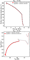Fig. B.1.

Evolution of average equatorial rotation velocity for a single 24 M_⊙ star with $v_{rot}^{ini}$ $v_{\mathrm{rot}}^{\mathrm{ini}}$ = 200 km s⁻¹ adopting different mesh_delta_coeff and time_delta_coeff parameters (top panel). The tracks continues only up to the terminal-age evolutionary phase. Bottom panel: HR diagram for the same model that continues until the end of the He-core burning phase.

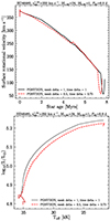Fig. B.2.

Same as Figure B.1, but for the HD 46485 system by taking into account the POSYDON structure dependent tidal synchronization prescription.

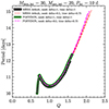Fig. B.3.

Period as a function of the mass ratio for a system initially defined as M_don, ini = 30 M_⊙, M_acc, ini = 20 M_⊙, and P_ini = 10 d. The distribution includes the MESA default and POSYDON tidal synchronization prescriptions.

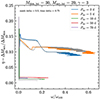Fig. B.4.

Mass transfer efficiency as a function of the angular velocity for the various initial periods of a given system (by taking into account the POSYDON tidal synchronization prescription). The gray points represent the model with the mesh_delta_coeff and time_delta_coeff equal to 1 and the "MESA default" tidal synchronization prescription.

Appendix C: Different formalisms of defining the tidal E₂ coefficient

To emphasize how the strengths of tides are sensitive to the adopted underlying physics we calculated the synchronization timescales (t_sync) for one of our stars where such differences are the most prominent because of the short orbital period (i.e. HD 191495, P ∼ 3.6 d). We illustrate in Figure C.1 how the synchronization timescale varies within the entire duration of the MS as a function of the radius of the primary component. The observed significant difference in t_sync for a given radius of the star (that also represents the evolutionary stage on the MS) occurs because of the different ways of calculating the E₂ coefficient which is important for calculating the timescale of synchronization for dynamical tides (regime of tides in the stellar radiative envelopes, (1/t_{sync, radiative} ∼ E₂). Indeed, as it addopted in Hurley et al. (2002, "MESA default" prescriprions) E₂ = 1.592 × 10⁻⁹(M/M_⊙)^2.84, while in Qin et al. (2018, "POSYDON" formalims for H-rich stars): E₂ = 10^−0.42(R_conv/R)^7.5. As we can see, in the "MESA default" prescription the E₂ parameter depends only on the entire mass of a star, while in the POSYDON formalism it depends on the stellar radius and the radius of the convective core (R_conv). Thus, the differences in resulting synchronization timescales which are presented in Figure C.1 occur because in the POSYDON prescription the E₂ is very sensitive to the size of the convective zone, especially taking into account that the ratio of R_conv/R is in a power of 7.5. In this test, we are illustrating how tidal interactions are sensitive to the adopted physics of tides and the evolutionary stage of the stars especially in massive binaries with an extended radiative envelope. Thus, while modeling the evolution of massive binaries, we suggest using the POSYDON tides formalism based on Qin et al. (2018) study.

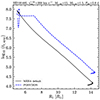Fig. C.1.

Synchronization timescale as a function of the primary component radius of HD 191495 system by assuming the MESA default (sync_type = "Hut_rad") and POSYDON (sync_type = "structure_dependent") tidal prescriptions.

Appendix D: Synchronization and circularization of the orbits

In Figure D.1 we present the evolution of surface average angular velocity for the three studied systems when assuming $v_{rot}^{ini}$ $v_{\mathrm{rot}}^{\mathrm{ini}}$ = 1 km s⁻¹. We illustrate its behavior by using different tides prescription, namely sync_type = "Hut_rad" (Hut 1980; Hurley et al. 2002), sync_type = "structure_dependent" (Qin et al. 2018), and no tidal interactions at all. The synchronization angular velocity is calculated as ω_sync = 2π/P. Where, P is the orbital period of the system that represents the orbit variations by assuming sync_type = "Hut_rad".

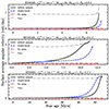Fig. D.1.

Evolution of surface average angular rotational velocity for our three program stars by taking into account different tidal synchronization prescriptions (assuming $v_{rot}^{1, ini}$ $v_{\mathrm{rot}}^{\mathrm{1, ini}}$ = 1 km s⁻¹). "MESA default" refers to the radiative envelope tidal synchronization prescription (sync_type = "Hut_rad"), and "POSYDON" to the structure dependent prescription.

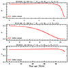Fig. D.2.

Evolution of eccentricity for our three stars assuming initial eccentricity equal to 0.5. "MESA default" refers to the sync_type = "Hut_rad" tidal synchronization prescription.

In order to investigate the typical circularization timescale for our system, we used circ_type = "Hut_rad" for both components which is based on the circularization timescales for radiative envelopes following Hurley et al. (2002). We assumed an initial eccentricity equal to 0.5.

All Tables

Table 1.

Basic physical and orbital parameters of three fast-rotating SB1 systems that have been investigated by Nazé et al. (2023).

In the text

Table 2.

Basic physical and orbital parameters for systems with a known fast-rotating OB star, extreme mass ratio, and short periods.

In the text

All Figures

	Fig. 1. Location in the HR diagram of the Galactic OB fast rotators studied in Britavskiy et al. (2023) and Nazé et al. (2023). Apparently single, binary, and runaway fast rotators are marked by specific symbols. Nonrotating evolutionary tracks represent the main-sequence stage of a single-star evolution at solar metallicity for different initial masses.
In the text

Fig. 2.

Evolution of equatorial surface rotational velocity of a single 24 M_⊙ star for different values of initial rotational velocity by assuming the formalism of the Vink et al. (2001) stellar wind model (solid lines) and the Björklund et al. (2023) wind model (dashed lines). In addition, tracks without the Spruit – Tayler dynamo mechanism (dotted-dashed lines) and the tracks assumed Fuller et al. (2019) AM transport (dotted lines) are added for reference. The tracks represent only the main-sequence stage up to terminal-age evolutionary phase. The error bars represent the observed position of HD 46485, whose primary has comparable mass.

In the text

Fig. 3.

Evolution of equatorial and synchronization surface rotational velocity for our three program systems by taking into account different tidal synchronization prescriptions. “MESA default” refers to the radiative envelope tidal synchronization (“Hut_rad” prescription), and “POSYDON” to the structure dependent prescription. We emphasize that different scales for the axes of each panel are used due to the different rotation rates, stellar masses, and thus lifetimes of the systems.

In the text

	Fig. 4. Same as Fig. 3 but assuming $v_{rot}^{1, ini}$ $v_{\mathrm{rot}}^{\mathrm{1,ini}}$ = 1 km s⁻¹. The gray dashed lines represent the evolution of synchronization rotational velocity for each system.
In the text

Fig. 5.

Evolution of the orbital period of HD 25631 for different values of the initial rotational velocity (including initially synchronized rotation for a given P_ini). The tracks stop at the onset of Roche lobe overflow of the primary star. When this occurs during its main-sequence (case A) we mark it by dots, conversely, if this happens after TAMS (gray dashed line) in a case B, we mark it with crosses. For reference, the inset shows the HR diagram around TAMS, where the beginning of the RLOF phases are marked by thick black outlines. The red horizontal line visualizes the initial value of the orbital period. In these simulations we used the sync_type = “Hut_rad” tidal prescription.

In the text

	Fig. 6. Efficiency of the CE process α_CE, with a different fraction of thermal energy α_th for our three targets (see text for details). In order to define the zone of the stellar core we indicated the mass fraction of X(¹H) by the gray line, linked to the right y-axis.
In the text

Fig. 7.

Orbital period vs. mass ratio relation for six cases of initial orbital periods (1.25, 3, 5, 10, 50, and 70 days) and masses M_don, ini = 30 M_⊙ and M_acc, ini = 20 M_⊙. Different tidal synchronization prescription regimes i.e. sync_type = “Hut_rad” (MESA default) and sync_type = “structure_dependent” (POSYDON) are presented. In addition, different fractions of mass lost from circumbinary toroid (via changing the mass transfer efficiency parameters δ and γ, see text for details) are shown. The cases with γ = 0 refer to the conservative mass transfer scenario. The RLOF phases are marked by a bold line. Filled and open circles indicate the reasons of track termination: both stars filled their Roche lobes or numerical convergence problem, respectively. In the case of 1.25 day configuration, both stars filled their RL almost simultaneously and we consider that all tracks indicate a subsequent merging.

In the text

	Fig. 8. Mass transfer efficiency (η) as a function of the surface average angular velocity for the various initial periods of a given system.
In the text

Fig. 9.

Minimum initial inner binary separation min(a_in) to prevent RLOF at periastron at ZAMS (i.e., R₁(m₁)≤R_RL, 1 and R₂(m₂)≤R_RL, 2) as a function of the inner binary mass ratio q_in = m₂/m₁ and eccentricity e_in for HD 45485 (top), HD 191495 (middle), and HD 25631 (bottom). The red solid lines mark the present-day observed separation, corresponding to the evolved post-merger a_out in the merger-in-a-triple scenario, while the black area in the bottom left corners corresponds the unphysical region with initial inner binary separation with R_i(m_i)≤R_RL, i. In the bottom row, the boundary of this unphysical region has a kink caused by the change of slope in the assumed mass–radius relation: HD 25631 primary mass is M₁ ≃ 7 M_⊙, so for q_in ≲ 0.2 (the exact threshold depends on f_Δ), the expected values of m₂ are sufficiently low that the exponent ξ in the R_ZAMS ≡ R_ZAMS(m) changes. For the right column with f_Δ ≠ 0, our assumptions based on the Blaauw (1961) approximation may be inconsistent (see Sect. 5).

In the text

Fig. 10.

Vast majority of triple systems compatible with the “merger in a triple” scenario has a probability of being dynamically unstable ≳90%. For each observed binary, we show the fraction of compatible putative triple progenitors that has a probability of being disrupted larger than the x coordinate according to the “ghost orbit” method of Vynatheya et al. (2023). Orange and blue curves correspond to the two values of fractional mass loss at merger f_Δ = 0 and 1 assumed. The distribution is marginalized over all parameters defining the architecture of the triples compatible with the present-day binaries (see text).

In the text

Fig. B.1.

Evolution of average equatorial rotation velocity for a single 24 M_⊙ star with $v_{rot}^{ini}$ $v_{\mathrm{rot}}^{\mathrm{ini}}$ = 200 km s⁻¹ adopting different mesh_delta_coeff and time_delta_coeff parameters (top panel). The tracks continues only up to the terminal-age evolutionary phase. Bottom panel: HR diagram for the same model that continues until the end of the He-core burning phase.

In the text

	Fig. B.2. Same as Figure B.1, but for the HD 46485 system by taking into account the POSYDON structure dependent tidal synchronization prescription.
In the text

	Fig. B.3. Period as a function of the mass ratio for a system initially defined as M_don, ini = 30 M_⊙, M_acc, ini = 20 M_⊙, and P_ini = 10 d. The distribution includes the MESA default and POSYDON tidal synchronization prescriptions.
In the text

	Fig. B.4. Mass transfer efficiency as a function of the angular velocity for the various initial periods of a given system (by taking into account the POSYDON tidal synchronization prescription). The gray points represent the model with the `mesh_delta_coeff` and `time_delta_coeff` equal to 1 and the "MESA default" tidal synchronization prescription.
In the text

	Fig. C.1. Synchronization timescale as a function of the primary component radius of HD 191495 system by assuming the MESA default (`sync_type = "Hut_rad"`) and POSYDON (`sync_type = "structure_dependent"`) tidal prescriptions.
In the text

Fig. D.1.

Evolution of surface average angular rotational velocity for our three program stars by taking into account different tidal synchronization prescriptions (assuming $v_{rot}^{1, ini}$ $v_{\mathrm{rot}}^{\mathrm{1, ini}}$ = 1 km s⁻¹). "MESA default" refers to the radiative envelope tidal synchronization prescription (sync_type = "Hut_rad"), and "POSYDON" to the structure dependent prescription.

In the text

	Fig. D.2. Evolution of eccentricity for our three stars assuming initial eccentricity equal to 0.5. "MESA default" refers to the `sync_type = "Hut_rad"` tidal synchronization prescription.
In the text

Current usage metrics show cumulative count of Article Views (full-text article views including HTML views, PDF and ePub downloads, according to the available data) and Abstracts Views on Vision4Press platform.

Data correspond to usage on the plateform after 2015. The current usage metrics is available 48-96 hours after online publication and is updated daily on week days.

Initial download of the metrics may take a while.

[1] Abbott, R., Abbott, T. D., Acernese, F., et al. 2023, Phys. Rev. X, 13, 041039 [Google Scholar]

[2] Abdul-Masih, M., Escorza, A., Menon, A., Mahy, L., & Marchant, P. 2022, A&A, 666, A18 [NASA ADS] [CrossRef] [EDP Sciences] [Google Scholar]

[3] Abt, H. A., & Moyd, K. I. 1973, ApJ, 182, 809 [NASA ADS] [CrossRef] [Google Scholar]

[4] Almeida, L. A., Sana, H., Taylor, W., et al. 2017, A&A, 598, A84 [NASA ADS] [CrossRef] [EDP Sciences] [Google Scholar]

[5] Angulo, C., Arnould, M., Rayet, M., et al. 1999, Nucl. Phys. A, 656, 3 [Google Scholar]

[6] Ballone, A., Costa, G., Mapelli, M., et al. 2023, MNRAS, 519, 5191 [NASA ADS] [CrossRef] [Google Scholar]

[7] Bastian, N., Kamann, S., Amard, L., et al. 2020, MNRAS, 495, 1978 [NASA ADS] [CrossRef] [Google Scholar]

[8] Bavera, S. S., Fragos, T., Qin, Y., et al. 2020, A&A, 635, A97 [NASA ADS] [CrossRef] [EDP Sciences] [Google Scholar]

[9] Björklund, R., Sundqvist, J. O., Puls, J., & Najarro, F. 2021, A&A, 648, A36 [EDP Sciences] [Google Scholar]

[10] Björklund, R., Sundqvist, J. O., Singh, S. M., Puls, J., & Najarro, F. 2023, A&A, 676, A109 [NASA ADS] [CrossRef] [EDP Sciences] [Google Scholar]

[11] Blaauw, A. 1961, Bull. Astron. Inst. Neth., 15, 265 [NASA ADS] [Google Scholar]

[12] Blaauw, A. 1993, in Massive Stars: Their Lives in the Interstellar Medium, eds. J. P. Cassinelli, & E. B. Churchwell, ASP Conf. Ser., 35, 207 [NASA ADS] [Google Scholar]

[13] Blagorodnova, N., Klencki, J., Pejcha, O., et al. 2021, A&A, 653, A134 [NASA ADS] [CrossRef] [EDP Sciences] [Google Scholar]

[14] Bodensteiner, J., Shenar, T., & Sana, H. 2020, A&A, 641, A42 [NASA ADS] [CrossRef] [EDP Sciences] [Google Scholar]

[15] Bodensteiner, J., Sana, H., Dufton, P. L., et al. 2023, A&A, 680, A32 [NASA ADS] [CrossRef] [EDP Sciences] [Google Scholar]

[16] Boersma, J. 1961, Bull. Astron. Inst. Neth., 15, 291 [NASA ADS] [Google Scholar]

[17] Bragança, G. A., Daflon, S., Cunha, K., et al. 2012, AJ, 144, 130 [CrossRef] [Google Scholar]

[18] Britavskiy, N., Simón-Díaz, S., Holgado, G., et al. 2023, A&A, 672, A22 [NASA ADS] [CrossRef] [EDP Sciences] [Google Scholar]

[19] Brott, I., Evans, C. J., Hunter, I., et al. 2011, A&A, 530, A116 [NASA ADS] [CrossRef] [EDP Sciences] [Google Scholar]

[20] Buchler, J. R., & Yueh, W. R. 1976, ApJ, 210, 440 [NASA ADS] [CrossRef] [Google Scholar]

[21] Callister, T. A., Haster, C.-J., Ng, K. K. Y., Vitale, S., & Farr, W. M. 2021, ApJ, 922, L5 [NASA ADS] [CrossRef] [Google Scholar]

[22] Carrier, F., Burki, G., & Burnet, M. 2002, A&A, 385, 488 [NASA ADS] [CrossRef] [EDP Sciences] [Google Scholar]

[23] Cassisi, S., Potekhin, A. Y., Pietrinferni, A., Catelan, M., & Salaris, M. 2007, ApJ, 661, 1094 [NASA ADS] [CrossRef] [Google Scholar]

[24] Cazorla, C., Nazé, Y., Morel, T., et al. 2017, A&A, 604, A123 [NASA ADS] [CrossRef] [EDP Sciences] [Google Scholar]

[25] Chatzopoulos, E., Frank, J., Marcello, D. C., & Clayton, G. C. 2020, ApJ, 896, 50 [NASA ADS] [CrossRef] [Google Scholar]

[26] Chugunov, A. I., Dewitt, H. E., & Yakovlev, D. G. 2007, Phys. Rev. D, 76, 025028 [NASA ADS] [CrossRef] [Google Scholar]

[27] Claeys, J. S. W., Pols, O. R., Izzard, R. G., Vink, J., & Verbunt, F. W. M. 2014, A&A, 563, A83 [NASA ADS] [CrossRef] [EDP Sciences] [Google Scholar]

[28] Claret, A., & Torres, G. 2018, ApJ, 859, 100 [Google Scholar]

[29] Conti, P. S., & Ebbets, D. 1977, ApJ, 213, 438 [CrossRef] [Google Scholar]

[30] Cyburt, R. H., Amthor, A. M., Ferguson, R., et al. 2010, ApJS, 189, 240 [NASA ADS] [CrossRef] [Google Scholar]

[31] de Jager, C., Nieuwenhuijzen, H., & van der Hucht, K. A. 1988, A&AS, 72, 259 [NASA ADS] [Google Scholar]

[32] De Marco, O., Passy, J.-C., Moe, M., et al. 2011, MNRAS, 411, 2277 [CrossRef] [Google Scholar]

[33] de Mink, S. E., Langer, N., Izzard, R. G., Sana, H., & de Koter, A. 2013, ApJ, 764, 166 [Google Scholar]

[34] de Mink, S. E., Sana, H., Langer, N., Izzard, R. G., & Schneider, F. R. N. 2014, ApJ, 782, 7 [Google Scholar]

[35] den Hartogh, J. W., Eggenberger, P., & Deheuvels, S. 2020, A&A, 634, L16 [NASA ADS] [CrossRef] [EDP Sciences] [Google Scholar]

[36] Deschamps, R., Siess, L., Davis, P. J., & Jorissen, A. 2013, A&A, 557, A40 [NASA ADS] [CrossRef] [EDP Sciences] [Google Scholar]

[37] Dewi, J. D. M., & Tauris, T. M. 2000, A&A, 360, 1043 [NASA ADS] [Google Scholar]

[38] Dodd, J. M., Oudmaijer, R. D., Radley, I. C., Vioque, M., & Frost, A. J. 2024, MNRAS, 527, 3076 [Google Scholar]

[39] Dorozsmai, A., Toonen, S., Vigna-Gómez, A., de Mink, S. E., & Kummer, F. 2024, MNRAS, 527, 9782 [Google Scholar]

[40] Drout, M. R., Götberg, Y., Ludwig, B. A., et al. 2023, Science, 382, 1287 [NASA ADS] [CrossRef] [Google Scholar]

[41] Duchêne, G., & Kraus, A. 2013, ARA&A, 51, 269 [Google Scholar]

[42] Dufton, P. L., Langer, N., Dunstall, P. R., et al. 2013, A&A, 550, A109 [NASA ADS] [CrossRef] [EDP Sciences] [Google Scholar]

[43] Dunstall, P. R., Dufton, P. L., Sana, H., et al. 2015, A&A, 580, A93 [NASA ADS] [CrossRef] [EDP Sciences] [Google Scholar]

[44] Eggleton, P. P. 1983, ApJ, 268, 368 [Google Scholar]

[45] Ekström, S., Georgy, C., Eggenberger, P., et al. 2012, A&A, 537, A146 [Google Scholar]

[46] El-Badry, K., & Burdge, K. B. 2022, MNRAS, 511, 24 [NASA ADS] [CrossRef] [Google Scholar]

[47] El-Badry, K., & Quataert, E. 2021, MNRAS, 502, 3436 [NASA ADS] [CrossRef] [Google Scholar]

[48] El-Badry, K., Conroy, C., Quataert, E., et al. 2022, MNRAS, 516, 3602 [NASA ADS] [CrossRef] [Google Scholar]

[49] Ferguson, J. W., Alexander, D. R., Allard, F., et al. 2005, ApJ, 623, 585 [Google Scholar]

[50] Fragos, T., Andrews, J. J., Bavera, S. S., et al. 2023, ApJS, 264, 45 [NASA ADS] [CrossRef] [Google Scholar]

[51] Frémat, Y., Zorec, J., Hubert, A. M., & Floquet, M. 2005, A&A, 440, 305 [NASA ADS] [CrossRef] [EDP Sciences] [Google Scholar]

[52] Fuller, J., & Lu, W. 2022, MNRAS, 511, 3951 [NASA ADS] [CrossRef] [Google Scholar]

[53] Fuller, G. M., Fowler, W. A., & Newman, M. J. 1985, ApJ, 293, 1 [NASA ADS] [CrossRef] [Google Scholar]

[54] Fuller, J., Piro, A. L., & Jermyn, A. S. 2019, MNRAS, 485, 3661 [NASA ADS] [Google Scholar]

[55] Glebbeek, E., Gaburov, E., Portegies Zwart, S., & Pols, O. R. 2013, MNRAS, 434, 3497 [NASA ADS] [CrossRef] [Google Scholar]

[56] Gormaz-Matamala, A. C., Cuadra, J., Meynet, G., & Curé, M. 2023, A&A, 673, A109 [NASA ADS] [CrossRef] [EDP Sciences] [Google Scholar]

[57] Götberg, Y., de Mink, S. E., Groh, J. H., et al. 2018, A&A, 615, A78 [NASA ADS] [CrossRef] [EDP Sciences] [Google Scholar]

[58] Götberg, Y., Drout, M. R., Ji, A. P., et al. 2023, ApJ, 959, 125 [CrossRef] [Google Scholar]

[59] Han, Z., Podsiadlowski, P., & Eggleton, P. P. 1995, MNRAS, 272, 800 [NASA ADS] [Google Scholar]

[60] Harmanec, P., Koubský, P., Nemravová, J. A., et al. 2015, A&A, 573, A107 [NASA ADS] [CrossRef] [EDP Sciences] [Google Scholar]

[61] Heger, A., Langer, N., & Woosley, S. E. 2000, ApJ, 528, 368 [NASA ADS] [CrossRef] [Google Scholar]

[62] Hendriks, D. D., & Izzard, R. G. 2023, MNRAS, 524, 4315 [NASA ADS] [CrossRef] [Google Scholar]

[63] Herwig, F. 2000, A&A, 360, 952 [NASA ADS] [Google Scholar]

[64] Holgado, G., Simón-Díaz, S., Herrero, A., & Barbá, R. H. 2022, A&A, 665, A150 [NASA ADS] [CrossRef] [EDP Sciences] [Google Scholar]

[65] Huang, W., Gies, D. R., & McSwain, M. V. 2010, ApJ, 722, 605 [Google Scholar]

[66] Hurley, J. R., Tout, C. A., & Pols, O. R. 2002, MNRAS, 329, 897 [Google Scholar]

[67] Hut, P. 1980, A&A, 92, 167 [NASA ADS] [Google Scholar]

[68] Hut, P. 1981, A&A, 99, 126 [NASA ADS] [Google Scholar]

[69] Iaconi, R., & De Marco, O. 2019, MNRAS, 490, 2550 [Google Scholar]

[70] Iglesias, C. A., & Rogers, F. J. 1993, ApJ, 412, 752 [Google Scholar]

[71] Iglesias, C. A., & Rogers, F. J. 1996, ApJ, 464, 943 [NASA ADS] [CrossRef] [Google Scholar]

[72] Itoh, N., Hayashi, H., Nishikawa, A., & Kohyama, Y. 1996, ApJS, 102, 411 [NASA ADS] [CrossRef] [Google Scholar]

[73] Ivanova, N., Podsiadlowski, P., & Spruit, H. 2002, MNRAS, 334, 819 [NASA ADS] [CrossRef] [Google Scholar]

[74] Ivanova, N., Justham, S., Chen, X., et al. 2013, A&ARv, 21, 59 [Google Scholar]

[75] Ivanova, N., Justham, S., & Ricker, P. 2020, Common Envelope Evolution (Bristol: IOP Publishing) [Google Scholar]

[76] Jermyn, A. S., Bauer, E. B., Schwab, J., et al. 2023, ApJS, 265, 15 [NASA ADS] [CrossRef] [Google Scholar]

[77] Jerzykiewicz, M., Pigulski, A., Michalska, G., et al. 2021, MNRAS, 503, 5554 [Google Scholar]

[78] Ji, S., Fuller, J., & Lecoanet, D. 2023, MNRAS, 521, 5372 [NASA ADS] [CrossRef] [Google Scholar]

[79] Johnston, C. 2021, A&A, 655, A29 [NASA ADS] [CrossRef] [EDP Sciences] [Google Scholar]

[80] Johnston, C., Aimar, N., Abdul-Masih, M., et al. 2021, MNRAS, 503, 1124 [NASA ADS] [CrossRef] [Google Scholar]

[81] Kamann, S., Saracino, S., Bastian, N., et al. 2023, MNRAS, 518, 1505 [Google Scholar]

[82] Kazeroni, R., Guilet, J., & Foglizzo, T. 2017, MNRAS, 471, 914 [NASA ADS] [CrossRef] [Google Scholar]

[83] Keszthelyi, Z., Puls, J., & Wade, G. A. 2017, A&A, 598, A4 [NASA ADS] [CrossRef] [EDP Sciences] [Google Scholar]

[84] Kippenhahn, R., & Weigert, A. 1967, Z. Astrophys., 65, 251 [NASA ADS] [Google Scholar]

[85] Klencki, J., Nelemans, G., Istrate, A. G., & Chruslinska, M. 2021, A&A, 645, A54 [EDP Sciences] [Google Scholar]

[86] Kobulnicky, H. A., Kiminki, D. C., Lundquist, M. J., et al. 2014, ApJS, 213, 34 [Google Scholar]

[87] Kolb, U., & Ritter, H. 1990, A&A, 236, 385 [NASA ADS] [Google Scholar]

[88] Kounkel, M., Stassun, K. G., Hillenbrand, L. A., et al. 2023, AJ, 165, 182 [NASA ADS] [CrossRef] [Google Scholar]

[89] Lalande, F., & Trani, A. A. 2022, ApJ, 938, 18 [NASA ADS] [CrossRef] [Google Scholar]

[90] Langanke, K., & Martínez-Pinedo, G. 2000, Nucl. Phys. A, 673, 481 [NASA ADS] [CrossRef] [Google Scholar]

[91] Langer, N. 1998, A&A, 329, 551 [NASA ADS] [Google Scholar]

[92] Langer, N. 2012, ARA&A, 50, 107 [CrossRef] [Google Scholar]

[93] Langer, N., Yoon, S. C., Petrovic, J., & Heger, A. 2003, ArXiv e-prints [arXiv:astro-ph/0302232] [Google Scholar]

[94] Ledoux, P. 1947, ApJ, 105, 305 [NASA ADS] [CrossRef] [Google Scholar]

[95] Limongi, M., & Chieffi, A. 2018, ApJS, 237, 13 [NASA ADS] [CrossRef] [Google Scholar]

[96] Lombardi, J. C., Jr., Warren, J. S., Rasio, F. A., Sills, A., & Warren, A. R. 2002, ApJ, 568, 939 [NASA ADS] [CrossRef] [Google Scholar]

[97] Lorenzo, J., Negueruela, I., Baker, A. K. F. V., et al. 2014, A&A, 572, A110 [NASA ADS] [CrossRef] [EDP Sciences] [Google Scholar]

[98] Ma, L., & Fuller, J. 2023, ApJ, 952, 53 [CrossRef] [Google Scholar]

[99] MacFadyen, A. I., & Woosley, S. E. 1999, ApJ, 524, 262 [NASA ADS] [CrossRef] [Google Scholar]

[100] Maeder, A., & Meynet, G. 2000, A&A, 361, 159 [NASA ADS] [Google Scholar]

[101] Mahy, L., Sana, H., Shenar, T., et al. 2022, A&A, 664, A159 [NASA ADS] [CrossRef] [EDP Sciences] [Google Scholar]

[102] Mardling, R., & Aarseth, S. 1999, in The Dynamics of Small Bodies in the Solar System, A Major Key to Solar System Studies, eds. B. A. Steves, & A. E. Roy, NATO Adv. Study Inst. (ASI) Ser. C, 522, 385 [NASA ADS] [CrossRef] [Google Scholar]

[103] Mason, B. D., Hartkopf, W. I., Gies, D. R., Henry, T. J., & Helsel, J. W. 2009, AJ, 137, 3358 [Google Scholar]

[104] Mirouh, G. M., Hendriks, D. D., Dykes, S., Moe, M., & Izzard, R. G. 2023, MNRAS, 524, 3978 [NASA ADS] [CrossRef] [Google Scholar]

[105] Moe, M., & Di Stefano, R. 2015, ApJ, 801, 113 [NASA ADS] [CrossRef] [Google Scholar]

[106] Moe, M., & Di Stefano, R. 2017, ApJS, 230, 15 [Google Scholar]

[107] Mokiem, M. R., de Koter, A., Vink, J. S., et al. 2007, A&A, 473, 603 [NASA ADS] [CrossRef] [EDP Sciences] [Google Scholar]

[108] Nazé, Y., Rauw, G., Smith, M. A., & Motch, C. 2022, MNRAS, 516, 3366 [CrossRef] [Google Scholar]

[109] Nazé, Y., Britavskiy, N., Rauw, G., Labadie-Bartz, J., & Simón-Díaz, S. 2023, MNRAS, 525, 1641 [CrossRef] [Google Scholar]

[110] Neo, S., Miyaji, S., Nomoto, K., & Sugimoto, D. 1977, PASJ, 29, 249 [NASA ADS] [Google Scholar]

[111] Oda, T., Hino, M., Muto, K., Takahara, M., & Sato, K. 1994, At. Data Nucl. Data Tables, 56, 231 [NASA ADS] [CrossRef] [Google Scholar]

[112] Offner, S. S. R., Moe, M., Kratter, K. M., et al. 2023, in Protostars and Planets VII, eds. S. Inutsuka, Y. Aikawa, T. Muto, K. Tomida, & M. Tamura, ASP Conf. Ser., 534, 275 [NASA ADS] [Google Scholar]

[113] Packet, W. 1981, A&A, 102, 17 [NASA ADS] [Google Scholar]

[114] Paczynski, B. 1976, in Structure and Evolution of Close Binary Systems, eds. P. Eggleton, S. Mitton, & J. Whelan, 73, 75 [NASA ADS] [CrossRef] [Google Scholar]

[115] Pauli, D., Langer, N., Aguilera-Dena, D. R., Wang, C., & Marchant, P. 2022, A&A, 667, A58 [NASA ADS] [CrossRef] [EDP Sciences] [Google Scholar]

[116] Paxton, B., Bildsten, L., Dotter, A., et al. 2011, ApJS, 192, 3 [Google Scholar]

[117] Paxton, B., Cantiello, M., Arras, P., et al. 2013, ApJS, 208, 4 [Google Scholar]

[118] Paxton, B., Marchant, P., Schwab, J., et al. 2015, ApJS, 220, 15 [Google Scholar]

[119] Paxton, B., Schwab, J., Bauer, E. B., et al. 2018, ApJS, 234, 34 [NASA ADS] [CrossRef] [Google Scholar]

[120] Paxton, B., Smolec, R., Schwab, J., et al. 2019, ApJS, 243, 10 [Google Scholar]

[121] Penny, L. R., & Gies, D. R. 2009, ApJ, 700, 844 [Google Scholar]

[122] Perets, H. B., & Kratter, K. M. 2012, ApJ, 760, 99 [NASA ADS] [CrossRef] [Google Scholar]

[123] Petrovic, J., Langer, N., & van der Hucht, K. A. 2005, A&A, 435, 1013 [NASA ADS] [CrossRef] [EDP Sciences] [Google Scholar]

[124] Pols, O. R., & Marinus, M. 1994, A&A, 288, 475 [NASA ADS] [Google Scholar]

[125] Pols, O. R., Tout, C. A., Eggleton, P. P., & Han, Z. 1995, MNRAS, 274, 964 [Google Scholar]

[126] Potekhin, A. Y., & Chabrier, G. 2010, Contrib. Plasma Phys., 50, 82 [NASA ADS] [CrossRef] [Google Scholar]

[127] Preece, H. P., Hamers, A. S., Neunteufel, P. G., Schaefer, A. L., & Tout, C. A. 2022, ApJ, 933, 25 [NASA ADS] [CrossRef] [Google Scholar]

[128] Qin, Y., Fragos, T., Meynet, G., et al. 2018, A&A, 616, A28 [NASA ADS] [CrossRef] [EDP Sciences] [Google Scholar]

[129] Ramachandran, V., Hamann, W. R., Oskinova, L. M., et al. 2019, A&A, 625, A104 [NASA ADS] [CrossRef] [EDP Sciences] [Google Scholar]

[130] Ramírez-Agudelo, O. H., Simón-Díaz, S., Sana, H., et al. 2013, A&A, 560, A29 [NASA ADS] [CrossRef] [EDP Sciences] [Google Scholar]

[131] Ramírez-Agudelo, O. H., Sana, H., de Mink, S. E., et al. 2015, A&A, 580, A92 [NASA ADS] [CrossRef] [EDP Sciences] [Google Scholar]

[132] Ramírez-Tannus, M. C., Backs, F., de Koter, A., et al. 2021, A&A, 645, L10 [NASA ADS] [CrossRef] [EDP Sciences] [Google Scholar]

[133] Reig, P. 2011, Ap&SS, 332, 1 [Google Scholar]

[134] Renzo, M., & Götberg, Y. 2021, ApJ, 923, 277 [NASA ADS] [CrossRef] [Google Scholar]

[135] Renzo, M., Ott, C. D., Shore, S. N., & de Mink, S. E. 2017, A&A, 603, A118 [NASA ADS] [CrossRef] [EDP Sciences] [Google Scholar]

[136] Renzo, M., Zapartas, E., de Mink, S. E., et al. 2019, A&A, 624, A66 [NASA ADS] [CrossRef] [EDP Sciences] [Google Scholar]

[137] Renzo, M., Cantiello, M., Metzger, B. D., & Jiang, Y. F. 2020, ApJ, 904, L13 [NASA ADS] [CrossRef] [Google Scholar]

[138] Renzo, M., Callister, T., Chatziioannou, K., et al. 2021, ApJ, 919, 128 [NASA ADS] [CrossRef] [Google Scholar]

[139] Renzo, M., Zapartas, E., Justham, S., et al. 2023, ApJ, 942, L32 [NASA ADS] [CrossRef] [Google Scholar]

[140] Rivinius, T., Carciofi, A. C., & Martayan, C. 2013, A&ARv, 21, 69 [Google Scholar]

[141] Rogers, F. J., & Nayfonov, A. 2002, ApJ, 576, 1064 [Google Scholar]

[142] Rosen, A. L., Krumholz, M. R., & Ramirez-Ruiz, E. 2012, ApJ, 748, 97 [NASA ADS] [CrossRef] [Google Scholar]

[143] Sana, H., de Mink, S. E., de Koter, A., et al. 2012, Science, 337, 444 [Google Scholar]

[144] Sana, H., de Koter, A., de Mink, S. E., et al. 2013, A&A, 550, A107 [NASA ADS] [CrossRef] [EDP Sciences] [Google Scholar]

[145] Sana, H., Ramírez-Tannus, M. C., de Koter, A., et al. 2017, A&A, 599, L9 [NASA ADS] [CrossRef] [EDP Sciences] [Google Scholar]

[146] Saracino, S., Shenar, T., Kamann, S., et al. 2023, MNRAS, 521, 3162 [NASA ADS] [CrossRef] [Google Scholar]

[147] Saumon, D., Chabrier, G., & van Horn, H. M. 1995, ApJS, 99, 713 [NASA ADS] [CrossRef] [Google Scholar]

[148] Schneider, F. R. N., Langer, N., de Koter, A., et al. 2014, A&A, 570, A66 [NASA ADS] [CrossRef] [EDP Sciences] [Google Scholar]

[149] Schneider, F. R. N., Podsiadlowski, P., Langer, N., Castro, N., & Fossati, L. 2016, MNRAS, 457, 2355 [Google Scholar]

[150] Schneider, F. R. N., Ohlmann, S. T., Podsiadlowski, P., et al. 2019, Nature, 574, 211 [Google Scholar]

[151] Schneider, F. R. N., Ohlmann, S. T., Podsiadlowski, P., et al. 2020, MNRAS, 495, 2796 [NASA ADS] [CrossRef] [Google Scholar]

[152] Schürmann, C., Langer, N., Xu, X., & Wang, C. 2022, A&A, 667, A122 [NASA ADS] [CrossRef] [EDP Sciences] [Google Scholar]

[153] Sciarini, L., Ekström, S., Eggenberger, P., et al. 2024, A&A, 681, L1 [NASA ADS] [CrossRef] [EDP Sciences] [Google Scholar]

[154] Sen, K., Langer, N., Marchant, P., et al. 2022, A&A, 659, A98 [NASA ADS] [CrossRef] [EDP Sciences] [Google Scholar]

[155] Serna, J., Hernandez, J., Kounkel, M., et al. 2021, ApJ, 923, 177 [NASA ADS] [CrossRef] [Google Scholar]

[156] Shao, Y., & Li, X.-D. 2016, ApJ, 833, 108 [NASA ADS] [CrossRef] [Google Scholar]

[157] Siess, L., Izzard, R. G., Davis, P. J., & Deschamps, R. 2013, A&A, 550, A100 [NASA ADS] [CrossRef] [EDP Sciences] [Google Scholar]

[158] Simón-Díaz, S., & Herrero, A. 2014, A&A, 562, A135 [NASA ADS] [CrossRef] [EDP Sciences] [Google Scholar]

[159] Smith, N. 2014, ARA&A, 52, 487 [NASA ADS] [CrossRef] [Google Scholar]

[160] Soberman, G. E., Phinney, E. S., & van den Heuvel, E. P. J. 1997, A&A, 327, 620 [NASA ADS] [Google Scholar]

[161] Southworth, J., & Bowman, D. M. 2022, MNRAS, 513, 3191 [Google Scholar]

[162] Spruit, H. C. 1999, A&A, 349, 189 [NASA ADS] [Google Scholar]

[163] Spruit, H. C. 2002, A&A, 381, 923 [CrossRef] [EDP Sciences] [Google Scholar]

[164] Stassun, K. G., Torres, G., Johnston, C., et al. 2021, ApJ, 910, 133 [NASA ADS] [CrossRef] [Google Scholar]

[165] Stevens, D. J., Zhou, G., Johnson, M. C., et al. 2020, MNRAS, 499, 3775 [NASA ADS] [CrossRef] [Google Scholar]

[166] Sweet, P. A. 1950, MNRAS, 110, 548 [Google Scholar]

[167] Tayler, R. J. 1973, MNRAS, 165, 39 [NASA ADS] [Google Scholar]

[168] Timmes, F. X., & Swesty, F. D. 2000, ApJS, 126, 501 [NASA ADS] [CrossRef] [Google Scholar]

[169] Tokovinin, A. 2018, ApJS, 235, 6 [NASA ADS] [CrossRef] [Google Scholar]

[170] Tokovinin, A., & Moe, M. 2020, MNRAS, 491, 5158 [NASA ADS] [CrossRef] [Google Scholar]

[171] Toonen, S., Hamers, A., & Portegies Zwart, S. 2016, Comput. Astrophys. Cosmol., 3, 6 [NASA ADS] [CrossRef] [Google Scholar]

[172] Toonen, S., Portegies Zwart, S., Hamers, A. S., & Bandopadhyay, D. 2020, A&A, 640, A16 [NASA ADS] [CrossRef] [EDP Sciences] [Google Scholar]

[173] Vanbeveren, D. 1981, A&A, 95, 321 [NASA ADS] [Google Scholar]

[174] Vanbeveren, D. 1982, A&A, 105, 260 [NASA ADS] [Google Scholar]

[175] van den Heuvel, E. P. J., Portegies Zwart, S. F., & de Mink, S. E. 2017, MNRAS, 471, 4256 [Google Scholar]

[176] Vinciguerra, S., Neijssel, C. J., Vigna-Gómez, A., et al. 2020, MNRAS, 498, 4705 [NASA ADS] [CrossRef] [Google Scholar]

[177] Vink, J. S., de Koter, A., & Lamers, H. J. G. L. M. 2001, A&A, 369, 574 [NASA ADS] [CrossRef] [EDP Sciences] [Google Scholar]

[178] Vynatheya, P., Hamers, A. S., Mardling, R. A., & Bellinger, E. P. 2022, MNRAS, 516, 4146 [NASA ADS] [CrossRef] [Google Scholar]

[179] Vynatheya, P., Mardling, R. A., & Hamers, A. S. 2023, MNRAS, 525, 2388 [NASA ADS] [CrossRef] [Google Scholar]

[180] Wang, L., Gies, D. R., & Peters, G. J. 2018, ApJ, 853, 156 [Google Scholar]

[181] Wang, C., Langer, N., Schootemeijer, A., et al. 2020, ApJ, 888, L12 [NASA ADS] [CrossRef] [Google Scholar]

[182] Wang, L., Gies, D. R., Peters, G. J., et al. 2021, AJ, 161, 248 [Google Scholar]

[183] Wang, C., Hastings, B., Schootemeijer, A., et al. 2023a, A&A, 670, A43 [NASA ADS] [CrossRef] [EDP Sciences] [Google Scholar]

[184] Wang, L., Gies, D. R., Peters, G. J., & Han, Z. 2023b, AJ, 165, 203 [NASA ADS] [CrossRef] [Google Scholar]

[185] Webbink, R. F. 1984, ApJ, 277, 355 [NASA ADS] [CrossRef] [Google Scholar]

[186] Willems, B., & Kolb, U. 2004, A&A, 419, 1057 [NASA ADS] [CrossRef] [EDP Sciences] [Google Scholar]

[187] Wolff, S. C., Edwards, S., & Preston, G. W. 1982, ApJ, 252, 322 [NASA ADS] [CrossRef] [Google Scholar]

[188] Wolff, S. C., Strom, S. E., Dror, D., & Venn, K. 2007, AJ, 133, 1092 [Google Scholar]

[189] Xin, C., Renzo, M., & Metzger, B. D. 2022, MNRAS, 516, 5816 [NASA ADS] [CrossRef] [Google Scholar]

[190] Zahn, J. P. 1975, A&A, 41, 329 [NASA ADS] [Google Scholar]

[191] Zahn, J. P. 1977, A&A, 57, 383 [Google Scholar]

[192] Zhao, X., & Fuller, J. 2020, MNRAS, 495, 249 [CrossRef] [Google Scholar]

[193] Zorotovic, M., Schreiber, M. R., & Parsons, S. G. 2014, A&A, 568, L9 [NASA ADS] [CrossRef] [EDP Sciences] [Google Scholar]

Tracing the evolution of short-period binaries with super-synchronous fast rotators

1. Introduction

2. Sample of stars and the adopted methodology

3. Primordial rotation – Pre-interaction scenario

3.1. Method

3.2. Results and interpretation (effect of mass loss)

3.3. Tidal interaction

3.4. Future of the systems

4. Spin-up – post-interaction scenario

4.1. Method

4.2. Results and interpretation

5. Merger in a triple

6. Discussion

6.1. Observational context

6.2. Theoretical implications

7. Conclusions

Acknowledgments

References

Appendix A: MESA setup

Appendix B: Resolution tests

Appendix C: Different formalisms of defining the tidal E2 coefficient

Appendix D: Synchronization and circularization of the orbits

All Tables

All Figures

Appendix C: Different formalisms of defining the tidal E₂ coefficient