| Issue |
A&A
Volume 684, April 2024
|
|
|---|---|---|
| Article Number | A128 | |
| Number of page(s) | 10 | |
| Section | Cosmology (including clusters of galaxies) | |
| DOI | https://doi.org/10.1051/0004-6361/202347393 | |
| Published online | 11 April 2024 | |
B-mode polarization forecasts for GreenPol
1
Institute of Theoretical Astrophysics, University of Oslo, Blindern, Oslo, Norway
e-mail: This email address is being protected from spambots. You need JavaScript enabled to view it.
2
Department of Physics, University of California, Santa Barbara, CA, USA
3
Niels Bohr Institute, University of Copenhagen, Blegdamsvej 17, Copenhagen, Denmark
4
Discovery Center, University of Copenhagen, Niels Bohr Institute, Blegdamsvej 17, Copenhagen, Denmark
5
Department of Physics, University of Oxford, Denys Wilkinson Building, Keble Road, Oxford OX1 3RH, UK
6
School of Physics and Optoelectronics Engineering, Anhui University, 111 Jiulong Road, Hefei, Anhui 230601, PR China
7
Key Laboratory of Particle and Astrophysics, Institute of High Energy Physics, CAS, 19B YuQuan Road, Beijing 100049, PR China
8
San Diego Supercomputer Center, University of California San Diego, La Jolla, CA, USA
Received:
7
July
2023
Accepted:
24
January
2024
Abstract
We present tensor-to-scalar ratio forecasts for GreenPol, a hypothetical ground-based B-mode experiment aiming to survey the cleanest regions of the Northern Galactic Hemisphere at five frequencies between 10 and 44 GHz. Its primary science goal would be to measure large-scale cosmic microwave background (CMB) polarization fluctuations at multipoles ℓ ≲ 500, and thereby constrain the primordial tensor-to-scalar ratio r. The observations for the suggested experiment would take place at the Summit Station (72 ° 34N, 38 ° 27W) on Greenland, at an altitude of 3216 m above sea level. For this paper we simulated various experimental setups, and derived limits on the tensor-to-scalar ratio after CMB component separation using a Bayesian component separation implementation called Commander. When combining the proposed experiment with Planck HFI observations for constraining polarized thermal dust emission, we found a projected limit of r < 0.02 at 95% confidence for the baseline configuration. This limit is very robust with respect to a range of important experimental parameters, including sky coverage, detector weighting, foreground priors, among others. Overall, GreenPol would have the possibility to provide deep CMB polarization measurements of the Northern Galactic Hemisphere at low frequencies.
Key words: polarization / methods: statistical / Galaxy: structure / cosmic background radiation / cosmology: observations / radio continuum: general
© The Authors 2024
 Open Access article, published by EDP Sciences, under the terms of the Creative Commons Attribution License (https://creativecommons.org/licenses/by/4.0), which permits unrestricted use, distribution, and reproduction in any medium, provided the original work is properly cited.
This article is published in open access under the Subscribe to Open model. This email address is being protected from spambots. You need JavaScript enabled to view it. to support open access publication.
1. Introduction
The detection of primordial gravitational waves in the form of large-scale polarization B modes in the CMB ranks as one of the most important goals in current cosmology. To date, the two most stringent limits on the amplitude of these waves (typically quantified by the so-called tensor-to-scalar ratio r) have been r < 0.036 (Ade et al. 2021) and r < 0.032 (Tristram et al. 2022), both at 95% confidence.
Before BICEP2, Keck, and Planck, the main challenge associated with this types of measurements was simply achieving sufficient instrumental sensitivity. The predicted amplitude of inflationary polarization B modes corresponds to less than 1 μK fluctuations on degree angular scales, and quite possibly less than 10 nK, depending on the precise numerical value of r (see, e.g., Lyth & Riotto 1999, and references therein). For this reason, the latest generation of B-mode instruments typically deploy hundreds or thousands of detectors, simply in order to achieve sufficient raw instrumental sensitivity (e.g., Austermann et al. 2012; Ade et al. 2014; Inoue et al. 2016; Thornton et al. 2016).
However, after BICEP2, Keck, and Planck, this situation has changed dramatically (BICEP2/Keck Collaboration 2015). Because of so-called foreground contamination in the form of polarized synchrotron and thermal dust emission from the Milky Way (Planck Collaboration X 2016), it has now become abundantly clear that raw sensitivity alone no longer suffices in order to improve existing constraints by a significant factor. The focus has rather turned to removing the foreground contaminants to a precision better than the noise level. This topic is called CMB component separation, and it is one of the central research topics in CMB physics today.
In order to reliably distinguish between cosmological and astrophysical sky signals, two main issues are of particular importance when designing a new experiment, namely field selection and frequency coverage. First, as illustrated by the Planck polarization maps (Planck Collaboration X 2016), the amplitude of polarized Galactic foregrounds varies by orders of magnitudes over the sky. In order to make the overall analysis problem as simple as possible, it is wise to observe the cleanest possible regions on the sky (Planck Collaboration XXX 2016). Of course, this strategy has been adopted by most experiments of this type deployed to date; however, before Planck, only very crude estimates of the amplitude of polarized thermal dust had been available. After Planck, we have a much more complete picture of the situation. And in this new situation, an interesting question has emerged: while most previous experiments have targeted the cleanest region of the Southern Galactic Hemisphere, there are possible hints in the latest Planck measurements that selected regions of the Northern Galactic Hemisphere could exhibit even lower overall foreground contamination (Planck Collaboration X 2016; Planck Collaboration XXX 2016). If this is correct, then it is clearly of great interest to deploy high-sensitivity experiments in the Northern Hemisphere in the near future, to supplement the data from, for instance, QUIJOTE (Rubiño-Martín et al. 2010), C-BASS (Jones et al. 2018), S-PASS (Carretti et al. 2019), or even dedicated SKA surveys (Basu et al. 2019).
The second issue concerns frequency coverage. Traditionally, most high-sensitivity experiments have employed bolometers above 90 GHz, primarily because of their excellent white noise performance and small focal plane area footprint; it is simply easier to achieve a high sensitivity at these frequency channels. For a long time, the astrophysics complexity of the sky as observed at the corresponding frequencies was of a secondary concern. However, the latest Planck measurements have shown that the amplitude of polarized thermal dust, which dominates on frequencies above 70 GHz, is higher than what many expected only a few years prior (Ade et al. 2014; BICEP2/Keck Collaboration 2015; Planck Collaboration X 2016).
In this new “high-foreground” situation, many important questions are currently being addressed quantitatively within the community. One example addresses whether thermal dust emission exhibits a simpler or more complex morphology than synchrotron emission in the presence of small-scale turbulent magnetic fields (e.g., Cho & Lazarian 2002; von Hausegger et al. 2019; Kim et al. 2019). Another question is whether the steep spectral index of synchrotron emission (Tν ∝ ν−3) is helpful or detrimental for component separation purposes, compared to the flatter index of thermal dust emission (Tν ∝ ν1.5); a steeper index makes synchrotron emission inherently less degenerate with the CMB than thermal dust emission, since the CMB spectrum itself is flat. On the other hand, the steep index also implies larger absolute amplitudes at low frequencies. On the low frequency side, there have also been efforts to investigate whether the synchrotron emission follows a power law throughout the observed frequency range, or whether it should contain a curvature (e.g., Kogut 2012; de la Hoz et al. 2023). A third question is whether synchrotron or thermal dust emission correlate more strongly with the CMB signal for a given experimental setup; this can for instance happen if the frequency range is insufficient to properly fit a given component. Lastly, possible frequency decorrelation may be induced by the 3D spatial variation of the foreground properties within the Milky Way, which, if not properly taken into account, can leak into the CMB (e.g., Tassis & Pavlidou 2015; Chluba et al. 2017; Vacher et al. 2022, 2023; Azzoni et al. 2021, 2023; Mangilli et al. 2021).
The precise answers to these questions depend sensitively on what the true sky looks like, both at low and high frequencies. Unfortunately, while Planck has provided an excellent view of frequencies higher than 100 GHz, and both QUIJOTE and C-BASS provide strong constraints between 5 and 19 GHz, an even higher sensitivity is still warranted. In order to make robust progress on all of the above questions, it is therefore essential to deploy new high-sensitivity low-frequency experiments targeting large regions of the cleanest parts of the sky.
In the following, we describe a potential experiment aiming to do this, called GreenPol. If funded, this experiment will deploy five receivers between 10 and 44 GHz on multiple low-cost telescopes, with a map-level sensitivity that is about four times higher than the published QUIJOTE multifrequency instrument (MFI) maps in the range 10 − 20 GHz (Rubiño-Martín et al. 2023). We note however that QUIJOTE will also have a new version of the low frequency instrument called MFI2 with a plan to improve the sensitivity by a factor of 2 or 3. GreenPol will be based at the Summit Station at Greenland, at an altitude of 3216 m above sea level. This site offers several unique and attractive features, as described in greater detail in the next section, but for the purposes of the current discussion the most important is simply that it provides a direct and continuous view of the cleanest regions of the Northern Galactic Hemisphere.
A similar experiment which also targets the Northern Galactic Hemisphere has been examined in Araujo et al. (2014), where the instrument is a compact CMB polarimeter based on lumped-element kinetic inductance detectors (LEKIDs). Observations would in this case be made from Isi Station in Greenland, and at higher frequencies than GreenPol, namely 150, 210 and 267 GHz.
The goal of the current paper is to provide preliminary forecasts for GreenPol in terms of effective limits on the tensor-to-scalar ratio. These forecasts are derived from ideal and simplified simulations that account for foregrounds and white noise only, but not instrumental systematics. The rest of the paper is organized as follows: In Sect. 2, we provide a more detailed overview of the technical specifications of the proposed experiment and the site, and discuss various aspects related to possible scanning strategies. In Sect. 3, we describe the methodology used to produce the forecasts, both in terms of simulations and posterior mapping framework. In Sect. 4 we summarize our main results, before concluding in Sect. 5.
2. GreenPol overview
The GreenPol concept relies on combining existing and proven detector technology with a low-cost telescope design (Childers et al. 2005). The top section of Table 1 provides an overview of the default detector combinations that are currently being considered. For frequencies between 10 and 30 GHz, coherent detectors such as those using High Electron Mobility Transistor amplifiers (HEMTs) may be preferred as they provide a path to mitigation of the rapidly increasing earth and orbitally based Radio Frequency Interference sources (Barron et al. 2022; Hoyland et al. 2022) while at higher frequencies, low-noise bolometers (e.g., transition edge sensor (TES) bolometers) are preferred. The quoted HEMT noise equivalent temperature (NET) levels represent real values measured on the sky with in-hand detectors, while the bolometer values represent typical values obtained by similar experiments (Kermish et al. 2012; George et al. 2012; Thornton et al. 2016; Ade et al. 2015).
Summary of instrument properties (top section), model parameters (middle section), and experimental setups (bottom section).
The GreenPol optical system would be based on recently developed carbon fiber mirror technology developed at the University of California Santa Barbara (UCSB), allowing for both cheap and lightweight production of multiple telescopes (Childers et al. 2005). The numbers of horns per telescope listed in Table 1 correspond to an optical system with a 2.2 m primary and 0.9 m secondary mirror, allowing for 7 horns at 10 GHz, 40 horns at 44 GHz, and 320 horns at 143 GHz. The effective angular resolution is 18.2′ full width half maximum (FWHM) at 44 GHz.
As already noted, one of the most unique features of GreenPol is its deployment location at the Summit Station (72 ° 34N, 38 ° 27W) on Greenland (Andersen & Rasmussen 2006). At a latitude of 72°N, this site provides unique access to the Northern Galactic Hemisphere, which hitherto has been largely unexplored by suborbital high-sensitivity CMB experiments. Summit Station is also an observing site with potentially optimal seeing conditions in the winter, particularly with respect to precipitable water vapor (Suen et al. 2014), though it was found that summer conditions present significant weather challenges.
The basic scanning strategy envisioned for GreenPol is based on full revolution constant elevation scans. The boresight of the telescope swipes out a circle of constant elevation in horizon coordinates at any given time, while the sky rotation slowly moves this circle across the sky. The most important free parameter in this scanning strategy is the co-elevation (or opening) angle α, which is the angle between the zenith and the boresight; the larger this angle is, the bigger sky fraction will be observed. In this paper, we consider four specific choices of this angle, namely α = 10°, 20°, 30° and 65°, but we note that the real experiment will most likely consider a wide range of such angles, for instance observing one day at each elevation, in order to uniformize the overall scan pattern. Indeed, the α = 65° presented below represents precisely such a union of multiple co-elevation angles, and the actual value of 65° simply quantifies the largest angle in the observation set. Figure 1 shows outlines of the sky coverages for each of the above co-elevation angles, overplotted on the Planck synchrotron (top) and thermal dust (bottom) Stokes Q polarization amplitude maps, evaluated at 44 GHz. A latitude of 72°N allows for continuous observations of a single field on the sky, although due to the constant elevation scan there is a hole in the field at the celestial pole, which we for visualization purposes have dropped in this figure.
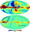 |
Fig. 1. Location of the GreenPol fields superimposed on the Planck Stokes Q synchrotron emission map (top panel) and the Planck Stokes Q thermal dust emission map (bottom panel), both evaluated at 44 GHz. The lines show the location of the 10° field (black), the 20° field (blue), the 30° field (white) and the 65° field (gray). |
Another powerful advantage of observations from a latitude of 72°N is the unique cross-linking properties, that is, multiple crossings over the same pixel from different orientations on the sky during a long integration scan. This is used to remove offsets estimated by minimizing the scatter among different measurements of each pixel and is extremely powerful for suppressing a wide range of instrumental systematic effects that are important for polarization measurements. The basic scanning strategy is identical to what was proposed in Araujo et al. (2014), and Fig. 8 (left panel) in that paper shows the scan path for 10 days of observations, selecting a different co-elevation angle each day.
In the summer of 2018 UCSB deployed a 10 GHz receiver with a 2.2 m primary mirror to Summit Station using a foldable design which allowed for storage in a standard ISO shipping container. This successfully demonstrated a method of shipping and quickly deploying a telescope in an extremely remote location, as well as the ability to quickly stow and redeploy the instrument in the face of changing weather conditions. The forecasting results show the potential for a larger experiment of this type with multiple telescopes and observing frequencies, which is made more feasible by the ability to ship and rapidly deploy fully functional telescopes to the desired observation site.
The primary goals of the mission were to assess the viability of the site for cosmological observations, as well as to conduct preliminary measurements and detect the Stokes Q and U components of the microwave foregrounds. However, the climate conditions during the summer deployment turned out to be more challenging than anticipated, with extended periods of overcast sky, freezing fog, wind, and blowing snow. Winter conditions at Summit Station may well be substantially better for observations, but this would need to be demonstrated on the ground before a full deployment. Notably, the observing strategy and analysis presented here do not require use of Summit Station, and there are other high quality Northern Hemisphere sites available (Marvil et al. 2006; Suen et al. 2014).
3. Forecast methodology
The goal of the current paper is to quantify the performance of an experiment such as GreenPol in terms of overall B-mode polarization sensitivity after component separation under ideal conditions. For this task, we combine simple simulations of the astrophysical sky with a well-established Bayesian component separation framework called Commander (Eriksen et al. 2004, 2008), and compare a range of different experimental setups in terms of their effective constraints on the tensor-to-scalar ratio.
3.1. Simulations
For our simulations, we adopt a simple model consisting of four components, namely CMB, synchrotron, and thermal dust emission, as well as instrumental noise. We model synchrotron emission with a simple power-law spectral energy density (SED) and thermal dust emission by a one-component modified blackbody SED (Planck Collaboration X 2016). We adopt thermodynamic temperature units throughout, and this simple model then takes the following form,
 (1)
(1)
 (2)
(2)
 (3)
(3)
 (4)
(4)
where dν(p) is the total simulated sky map at frequency ν and pixel p; s is the CMB signal; as and βs are the synchrotron amplitude (at a reference frequency of νs = 23 GHz) and spectral index; ad, βd and Td are the thermal dust amplitude (at a reference frequency of νd = 353 GHz), spectral index and temperature, respectively; γ(ν) is the conversion factor between Rayleigh-Jeans and thermodynamic temperatures for differential observations1; and n is instrumental noise.
Simulated CMB sky maps are generated using the HEALPix2 (Górski et al. 2005) facility called synfast, combined with a theoretical ΛCDM angular power spectrum computed with CAMB (Lewis et al. 2000) for various values of the tensor-to-scalar ratio and an optical depth of reionization of τ = 0.06. All other cosmological parameters are fixed at best-fit Planck values (Planck Collaboration XIII 2016).
For the synchrotron component, we adopt the Wilkinson Microwave Anisotropy Probe (WMAP) K-band (23 GHz) Stokes Q and U maps as a spatial template (Bennett et al. 2013), and a spatially constant spectral index of βs = −3.1 across our fields. Likewise, for thermal dust emission we adopt the Planck 353 GHz Stokes Q and U maps as a spatial template (Planck Collaboration I 2016), and spatially constant values of βd = 1.5 and Td = 21 K (Planck Collaboration X 2016). We note that while we do adopt spatially constant spectral indices in the simulation, no such assumptions are enforced or assumed in the analysis, but both βs and βd are fitted independently pixel-by-pixel. The thermal dust temperature is kept fixed on the input value in the fit, since this parameter is not constrained by the frequencies in question for GreenPol.
As a test of potential modeling errors, we also consider one case that includes polarized spinning dust in the input simulation, but not in the fitted model. The SED for the spinning dust component is taken to match the corresponding intensity SED for spinning dust as reported in Fig. 51 of Planck Collaboration X (2016), while the Planck 353 GHz thermal dust polarized amplitude map is adopted as a spatial template. Finally, we adopt a polarization fraction of 1%, consistent with current upper limits (e.g., Génova-Santos et al. 2015).
All input sky maps are downgraded to Nside = 64 and smoothed to a common resolution of 1° FWHM before co-addition. On top of this, we add Gaussian white noise modulated by the scanning strategy, with a root mean square (RMS) per pixel given by  , while properly accounting for smoothing; Nobs(p) is the number of observations in pixel p, computed by simulating the scan path of the instrument for one year of observations. The noise is assumed independent in Stokes Q and U.
For each considered experimental setup, we analyze 20 independent simulations with different CMB and noise realizations. All quoted results, unless specified otherwise, correspond to averages over these 20 realizations.
3.2. Posterior mapping
We extract an estimate of the tensor-to-scalar posterior distribution, P(r|d), using a Bayesian analysis framework called Commander (Eriksen et al. 2004, 2008). Throughout this paper, we use Commander1 (Eriksen et al. 2008), which is very well suited when it comes to exploring a diversity of cases like in this paper. This machinery has already been used extensively for similar types of analyses in the literature, both for real (e.g., Planck Collaboration X 2016) and simulated data (e.g., Armitage-Caplan et al. 2012; Remazeilles et al. 2016; Fuskeland et al. 2023). The latest Commander implementation, Commander3 (Galloway et al. 2023), is able to perform end-to-end analysis all the way from time ordered data to cosmological parameters, as demonstrated by the BeyondPlanck (BeyondPlanck Collaboration 2023) and Cosmoglobe (Watts et al. 2023) projects. However, this implementation also has a much higher computational cost than Commander1, and is not yet suitable for fast exploration of many experimental configurations as considered in this paper. In the following, we provide a brief summary of the main ideas, and refer the interested reader to the dedicated papers for full details.
In short, Commander implements a specific Markov chain Monte Carlo sampling algorithm for parametric component separation. In this approach, the first step is to map out the full joint posterior including all sky components, P(s, as, βs, ad, βd|d), and then constrain the tensor-to-scalar ratio posterior from the corresponding marginal CMB sky map posterior. The first step in this process is performed by a special technique called Gibbs sampling (e.g., Gelman et al. 2013), in which samples from the full posterior distribution are drawn by iteratively sampling from all relevant conditional distributions. For the purposes of the current paper, this can be summarized in the following three-step Gibbs sampler,
 (5)
(5)
 (6)
(6)
 (7)
(7)
where ← means sampling from the expression on the right hand side. For a full account of the sampling steps, see Eriksen et al. (2008). In short, we first sample all linear degrees of freedom (i.e., component amplitudes) jointly from a multivariate Gaussian, while all nonlinear parameters (i.e., spectral indices) are sampled iteratively by an explicit inversion sampler.
We run this iterative sampler until convergence, which typically requires 𝒪(105) samples for robust convergence. From the resulting CMB sky map samples we then compute the posterior mean CMB map,  , and effective noise covariance matrix, N, with elements
 (8)
(8)
 (9)
(9)
where brackets indicate average over samples. Finally, these sample averaged objects are fed into a standard Gaussian likelihood of the form
 (10)
(10)
where S(r) is the CMB signal covariance matrix evaluated for the appropriate value of r and the best-fit ΛCDM parameters described above. We adopt a uniform prior for all positive values of r, and the posterior is therefore numerically equal to the likelihood in Eq. (10). To map out this posterior, we simply map out Eq. (10) over a one-dimensional grid in r.
4. Results
With the above simulation and analysis pipeline, we are now ready to explore the effect of various experimental setups on our final constraints on the tensor-to-scalar ratio.
4.1. Baseline configuration
Our first simulation configuration represents the baseline against which all other configurations are compared. This setup adopts the SN10 observational strategy, resulting in a sky fraction of fsky = 0.06, and adopting signal-to-noise weighting for the GreenPol frequency bands, see Table 1. The foreground model includes synchrotron and thermal dust emission both in the simulation and in the analysis, with the product of uniform (−4.5 < βs < −1.5 and 1.0 < βd < 2.0) and Gaussian (βs ∼ 𝒩(−3.1, σβs = 0.1) and βd ∼ 𝒩(1.50, σβd = 0.05)) priors. The tensor-to-scalar ratio is fixed to r = 0, while all other cosmological parameters are set to the best-fit ΛCDM model described in Sect. 3.1.
In Fig. 2 we compare the true input maps (left column) with the reconstructed posterior mean maps (second column) for each free parameter for one simulation with this particular setup. We only show Stokes Q in this plot, since U looks qualitatively very similar. The third column shows their difference, while the fourth column shows the posterior RMS map as estimated by the Gibbs sampler; ideally, the maps in the third column should be consistent with Gaussian random noise with a standard deviation given by the fourth column. At least visually, this expectation appears to be met quite well, with no obvious signs of consistent correlated structures in the residual maps. Of course, since the fitted model matches the true signal, this is not surprising, but it still serves as an important self-consistency check.
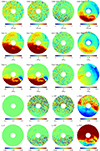 |
Fig. 2. Comparison of input maps (first column), reconstructed maps (second column), residual (output minus input) maps (third column), and posterior RMS maps (fourth column) for the baseline SN10 experimental setup. From top to bottom, rows show: (1) Stokes Q CMB in thermodynamic units, (2) Stokes Q synchrotron amplitude at 23 GHz in Rayleigh-Jeans (RJ) units, (3) Stokes Q thermal dust amplitude at 353 GHz in RJ units, (4) synchrotron spectral index, and (5) thermal dust spectral index. |
The structures of the posterior RMS maps also agree with our expectations. For instance, the uncertainty in the component amplitude parameters (CMB, synchrotron, and thermal dust) is larger where the foregrounds are bright, whereas the uncertainty in the spectral index parameters is smaller in the same region. For the CMB, this spatially varying standard deviation naturally down-weighs regions with bright foregrounds in the tensor-to-scalar ratio likelihood fit, serving effectively as a mild form of masking. Along the edges of the amplitude maps, the uncertainties are generally smaller because of the relatively higher number of observations per pixel due to the scanning pattern, this can be seen in the CMB and synchrotron RMS maps. For the thermal dust RMS map, the sharp features trace the Planck scanning strategy.
The black solid line in Fig. 3 shows the resulting marginal tensor-to-scalar ratio posterior distribution, averaged over 20 simulations. This distribution peaks at r = 0, in agreement with the input value, and has an upper 95% confidence limit of r = 0.017. This value thus represents a baseline comparison point against which we can compare other experimental setups.
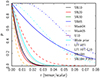 |
Fig. 3. Marginal tensor-to-scalar ratio posterior distributions for various experimental setups, averaged over 20 simulations. All setups, except SN10H and SN10H G10, contain the Planck HFI channels, and all except LFI HFI and LFI HFI G10, contains the 5 lowest GreenPol channels. |
Before doing that, however, it is interesting to understand at what level foreground marginalization degrades the overall results, compared to a CMB-only setup with the same sensitivity. To answer this question, we compare in Fig. 4 the upper 95% confidence limits averaged over 20 simulations with the corresponding 68% region error bars, as derived with four simple sky model variations, namely (1) CMB only; (2) CMB and thermal dust; (3) CMB and synchrotron; and (4) CMB, synchrotron, and thermal dust (all in addition to noise). The latter point thus corresponds directly to the baseline model. Overall, we see that all four models result in very similar constraints, with a very slight posterior degradation of about 10% due to synchrotron emission marginalization, but no measurable degradation due to thermal dust marginalization. The fact that the mean point is slightly lower in the CMB+dust model is due to the limited number of simulations, and is not statistically significant. This shows that the frequency band selection in the baseline configuration results in a robust component separation efficiency, achieving nearly optimal post-component separation results.
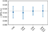 |
Fig. 4. Comparison of the upper 95% confidence limits of the tensor-to-scalar ratio posteriors for (1) CMB only; (2) CMB and thermal dust; (3) CMB and synchrotron; and (4) CMB, synchrotron, and thermal dust (in addition to noise), all evaluated for the baseline experiment configuration. Each point represents the mean of the 95% confidence limits evaluated from 20 simulations, and the error bar indicates the 68% region among the same simulations. The horizontal gray dashed line indicates the value for Case 4, representing the full model, SN10. The true input value is r = 0. |
As a bias test and sanity check on the baseline configuration, we have also analyzed a similar set of simulations, but this time with adopting a nonzero value of the tensor-to-scalar ratio of r = 0.05 and fixed spectral indices, σd = σs = 0; the latter choice is introduced because the mathematical problem then has an algebraically closed solution, which is useful for validation. The results from this calculation are shown in Fig. 5; as expected, the recovered posterior distribution is consistent with the input value. We note that the width of this distribution is larger for r = 0.05 than for r = 0, as expected due to cosmic variance.
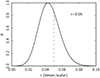 |
Fig. 5. Marginal tensor-to-scalar ratio posterior distribution for the case where r = 0.05 and fixed spectral index priors σd = σs = 0, averaged over 20 simulations. The vertical gray dashed line is the true value, r = 0.05. |
4.2. Configuration variations
We are now ready to explore the larger experimental parameter space, introducing variations around the baseline model SN10. In each case, we only focus on the resulting tensor-to-scalar ratio posterior distributions, and in particular on the upper 95% confidence limits, and not show individual sky maps for each; these look qualitatively similar to those shown in Fig. 2. In Table 2 all the different configuration variations are listed with check marks at the relevant GreenPol and Planck Low Frequency Instrument (LFI) and High Frequency Instrument (HFI) frequency channels, together with the resulting upper 95% confidence limits on r.
Upper 95% confidence limits (CL) of r and included frequency channels for each experimental configuration.
Sky fraction. In our first set of variations, we simply change the effective sky fraction, adopting opening angles of α = 20°, α = 30°, and α = 65°, corresponding to sky fractions of 0.11, 0.16 and 0.44, respectively. The cases are labeled SN20, SN30, and SN65. The posterior distributions obtained from these are shown as red, green and blue solid lines in Fig. 3, and the resulting upper 95% confidence limits are plotted with one sigma error bars in Fig. 6. Overall, we see that a larger sky fraction generally leads to weaker constraints on the tensor-to-scalar ratio, although for sky fractions up to 0.16 the effect is very marginal. For the largest sky fraction of 0.44, however, the effect is large, effectively reducing the detection power by a factor of four. The main reason for this dramatic increase is simply that for the largest opening angle, a relatively large fraction of the observation time is spent within the Galactic Plane, where the CMB constraints are relatively poor.
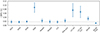 |
Fig. 6. Comparison of the upper 95% confidence limits of the tensor-to-scalar ratio r for various experimental setups. Each point represents the mean of the 95% confidence limits evaluated from 20 simulations, and the error bar indicates the 68% region among the same simulations. The horizontal gray dashed line is the value of the baseline configuration, SN10. The true input value for all these configurations is r = 0. |
Masking. To quantify the effect of masking on the smaller fields, we next consider two cases in which high-foreground pixels are simply removed from the analysis by an explicit mask. Two different masks are considered. Mask04 is defined by thresholding the Planck synchrotron polarization, resulting in a sky fraction of fsky = 0.73 for a full sky map, and fsky = 0.04 for our 10° field. The other mask, Mask05, is defined by thresholding the CMB posterior RMS map at 0.4 μK (and thus only removing pixels in the Stokes Q map), resulting in a sky fraction of fsky = 0.05 averaged over Stokes Q and U. The resulting posteriors are shown as dotted lines in Fig. 3, and the upper 95% confidence limits plotted in Fig. 6. As expected, the constraints degrade proportionally to the removed sky fraction.
Noise weighting. Next, we consider a different relative weighting between frequency channels. As described above, the baseline configuration adopts total signal-to-noise ratio weights for each frequency channel (i.e., number of detectors per band), which is qualitatively similar to Planck. In the next variation, we instead consider uniform weighting between frequencies, U10, as measured in units of telescope years. In terms of implementation strategy, this is easier to achieve, since each telescope can then be tuned to a specific frequency, and does not require multi-frequency optical elements. The resulting tensor-to-scalar ratio posterior distribution and upper 95% confidence limit are summarized in Figs. 3 and 6. Overall, this configuration performs very similar to the baseline configuration, suggesting that the specific choice of detector weights is not critical for the final results. This, of course, is not surprising, considering the stability of the CMB solution with respect to foregrounds that was demonstrated in Fig. 4.
Foreground priors. As a further test of foreground stability, we next consider the case in which the Gaussian priors on the spectral parameters are loosened (tripled), from σβs = 0.1 and σβd = 0.05 to σβs = 0.3 and σβd = 0.15, respectively. The resulting posterior distribution is plotted as a cyan solid curve in Fig. 3 (Wide prior), and the upper 95% confidence limit on the tensor-to-scalar ratio degrades by about 30%, from r < 0.020 to r < 0.025.
Comparison with other experiments. We now consider combinations of different data sets and frequencies. In the first case (LFI HFI), we simply replace all GreenPol frequencies with the three currently available Planck LFI frequencies at 30, 44 and 70 GHz. As seen in Fig. 6, this results in a mean upper 95% confidence limit on the tensor-to-scalar ratio of r < 0.08. Adding only the 10 GHz GreenPol channel to Planck LFI+HFI combination (LFI HFI G10) improves this limit to r < 0.07. In the third case, we replace the Planck HFI frequencies between 100 and 353 GHz with internal GreenPol bands at 90 and 143 GHz, SN10H; this results in a limit of r < 0.035. The fourth and last case (SN10H P353) is one where we add only the Planck 353 GHz channel to the full-range GreenPol configuration; this results in the tightest limit of all cases considered in this paper, resulting in a 95% confidence limit of r < 0.012. Overall, it is clear that internal high-frequency channels are not able to replace the Planck HFI data, and in particular the 353 GHz channel, in terms of sheer sensitivity, but they would be extremely valuable additions both in terms of final sensitivity and overall robustness with respect to instrumental systematics.
In Fig. 7 we show the posterior RMS maps for synchrotron and thermal dust spectral indices for the Wide prior setup containing five low GreenPol channels plus HFI (top) and the Planck only setup, (bottom). Both setups are sampled using wide priors, σβs = 0.3 and σβd = 0.15. Here we clearly see that the Planck setup is totally prior dominated with regard to the synchrotron spectral index, while the setup containing low GreenPol frequencies instead of LFI, is able to get good constraints on the spectral index. For the case of thermal dust spectral index, both setups are prior dominated at the highest latitudes where the signal is low. In fact the setup containing the low GreenPol frequencies is even a little bit less prior dominated than the Planck only setup.
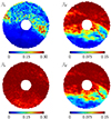 |
Fig. 7. Comparison of RMS maps of the synchrotron (left column) and dust (right column) spectral indices for two different configurations. Top: posterior RMS maps for the Wide prior setup with the 5 low GreenPol frequencies plus Planck HFI. Bottom: posterior RMS maps for the Planck LFI HFI setup sampled with a wide prior. |
Modeling errors. Finally, we consider a case with an explicit mismatch between the data and the fitted model, which is generated by adding a spinning dust component with a polarization fraction of 1% to the input simulation. The resulting tensor-to-scalar ratio posterior is shown in the top panel of Fig. 8. In this case, the result is formally a spurious foreground-induced detection of a tensor-to-scalar ratio of r = 0.16 ± 0.04. The bottom panel of Fig. 8 shows the goodness of fit, the χ2 map (Stokes Q) resulting from this analysis; the corresponding reduced χ2 is 1.22 ± 0.02, indicating the presence of a strong model mismatch as opposed to being unity as in all the previous cases. Thus, this spurious detection would be rejected internally by the component separation process. When we apply a mask on the foreground dominated part, Mask04, indicated by the white line on the χ2 map, the detection is replaced by a value that fits a vanishing r, with a 95% confidence limit of r < 0.03. The red dashed line in Fig. 8 shows the corresponding posterior curve.
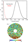 |
Fig. 8. Results for the modeling errors case. Top: marginal tensor-to-scalar posterior distribution for a model mismatch of adding a spinning dust component in the simulation. The dashed red line shows the posterior after the mask, Mask04, is applied. Bottom: corresponding Stokes Qχ2 map for one arbitrary sample. The white line indicates the masked-out region. |
5. Conclusions
In this paper, we have performed a preliminary sensitivity analysis for GreenPol, a hypothetical new ground-based CMB B-mode polarization experiment. This experiment is designed to observe the Northern Galactic Hemisphere from the Summit site on Greenland; at an altitude of 3216 m above sea level and a latitude of 72°N. This site exhibits excellent observing conditions for future CMB polarization experiments, both in terms of atmospheric transmission and observing strategies. GreenPol would then primarily observe at low-frequencies, between 10 and 44 GHz, and combine the resulting data with observations from the Planck HFI instrument and/or internal observations at 90 and 143 GHz. The proposed GreenPol detector technology and unique observing site makes the experiment complementary to existing efforts, most of which focus on the Southern Galactic Hemisphere.
The primary goal of the current paper is to quantify the sensitivity of GreenPol in terms of constraints on the tensor-to-scalar ratio after component separation. We have done this by analyzing simplified and controlled simulations within a well-established Bayesian component separation framework called Commander. We find that the constraints on synchrotron emission improve when adding the low frequency GreenPol data to the Planck data. We expect that this trend will become even more important when also accounting for spatial variations in the spectral index and curvature; however, exploring this is beyond the scope of this paper.
To summarize, our main conclusions are the following:
-
When combined with Planck HFI observations, GreenPol would constrain the tensor-to-scalar ratio to r < 0.02 at 95% confidence limit. This is competitive with existing constraints. For instance, the current best constraint from BICEP2+Keck+Planck is r < 0.032 (Tristram et al. 2022).
-
The value of r < 0.02 is robust with respect to specific details in the experimental configuration; neither sky fraction (up to a certain limit), detector weighting, nor foreground priors affect this value significantly. Indeed, the frequency layout proposed for GreenPol provides a foreground stability that yields constraints on the tensor-to-scalar ratio that exceeds the CMB-only prediction by only about 10%.
-
For cross-validation purposes, the Planck HFI observations could be replaced with internal observations at 90 and 143 GHz. This carries a cost of about 100% in constraining power, increasing the tensor-to-scalar ratio limit to r < 0.035. However, having two fully independent data sets available for thermal dust reconstruction would also greatly improve our ability to reject a potential false detection due to instrumental systematic effects.
 where x = hν/kBTCMB; h is Planck’s constant, and kB is Boltzmann’s constant.
Acknowledgments
Some of the results in this paper have been derived using the healpy (Zonca et al. 2019) and HEALPix (Górski et al. 2005) packages. We are grateful to Villum Fond for support of the Deep Space project. This work has received funding from the European Union’s Horizon 2020 research and innovation programme under grant agreement numbers 819478 (ERC; COSMOGLOBE) and 772253 (ERC; BITS2COSMOLOGY). This work is supported by the Research Council of Norway under grant agreement number 230947. This work is also supported in part by the National Key R&D Program of China (2021YFC2203100, 2021YFC2203104) and the Anhui project Z010118169. S.v.H. acknowledges funding from the Beecroft Trust. A.K., P.M. and P.L. were supported by the Niels Bohr Institute and the Villum Foundation. We would like to thank the US NSF and the staff at Summit Station for excellent support during our observing campaign.
References
- Ade, P. A. R., Aikin, R. W., Amiri, M., et al. 2014, ApJ, 792, 62 [CrossRef] [Google Scholar]
- Ade, P. A. R., Aikin, R. W., Amiri, M., et al. 2015, ApJ, 812, 176 [NASA ADS] [CrossRef] [Google Scholar]
- Ade, P. A. R., Ahmed, Z., Amiri, M., et al. 2021, Phys. Rev. Lett., 127, 151301 [NASA ADS] [CrossRef] [Google Scholar]
- Andersen, M. I., & Rasmussen, P. K. 2006, IAU Spec. Session, 7, 11 [NASA ADS] [Google Scholar]
- Araujo, D. C., Ade, P. A. R., Bond, J. R., et al. 2014, Proc. SPIE., 9153, 91530W [NASA ADS] [CrossRef] [Google Scholar]
- Armitage-Caplan, C., Dunkley, J., Eriksen, H. K., & Dickinson, C. 2012, MNRAS, 424, 1914 [NASA ADS] [CrossRef] [Google Scholar]
- Austermann, J. E., Aird, K. A., Beall, J. A., et al. 2012, Proc. SPIE, 8452, 84521E [NASA ADS] [CrossRef] [Google Scholar]
- Azzoni, S., Abitbol, M. H., Alonso, D., et al. 2021, JCAP, 2021, 047 [CrossRef] [Google Scholar]
- Azzoni, S., Alonso, D., Abitbol, M. H., et al. 2023, JCAP, 2023, 035 [CrossRef] [Google Scholar]
- Barron, D. R., Bender, A. N., Birdwell, I. E., et al. 2022, Proc. SPIE, 12190, 1219002 [NASA ADS] [Google Scholar]
- Basu, A., Schwarz, D. J., Klöckner, H. R., von Hausegger, S., et al. 2019, MNRAS, 488, 1618 [NASA ADS] [CrossRef] [Google Scholar]
- Bennett, C. L., Larson, D., Weiland, J. L., et al. 2013, ApJS, 208, 20 [Google Scholar]
- BeyondPlanck Collaboration (Andersen, K. J., et al.) 2023, A&A, 675, A1 [Google Scholar]
- BICEP2/Keck Collaboration, Planck Collaboration (Ade, P. A. R., et al.) 2015, Phys. Rev. Lett., 114, 101301 [NASA ADS] [CrossRef] [Google Scholar]
- Carretti, E., Haverkorn, M., Staveley-Smith, L., et al. 2019, MNRAS, 489, 2330 [Google Scholar]
- Childers, J., Bersanelli, M., Figueiredo, N., et al. 2005, ApJS, 158, 124 [NASA ADS] [CrossRef] [Google Scholar]
- Chluba, J., Hill, J. C., & Abitbol, M. H. 2017, MNRAS, 472, 1195 [NASA ADS] [CrossRef] [Google Scholar]
- Cho, J., & Lazarian, A. 2002, ApJ, 575, L63 [Google Scholar]
- de la Hoz, E., Barreiro, R. B., Vielva, P., et al. 2023, MNRAS, 519, 3504 [NASA ADS] [CrossRef] [Google Scholar]
- Eriksen, H. K., O’Dwyer, I. J., Jewell, J. B., et al. 2004, ApJS, 155, 227 [Google Scholar]
- Eriksen, H. K., Jewell, J. B., Dickinson, C., et al. 2008, ApJ, 676, 10 [Google Scholar]
- Fuskeland, U., Aumont, J., Aurlien, R., et al. 2023, A&A, 676, A42 [NASA ADS] [CrossRef] [EDP Sciences] [Google Scholar]
- Galloway, M., Andersen, K. J., Aurlien, R., et al. 2023, A&A, 675, A3 [NASA ADS] [CrossRef] [EDP Sciences] [Google Scholar]
- Gelman, A., Carlin, J. B., Stern, H. S., et al. 2013, Bayesian Data Analysis, 3rd edn. (London: Chapman& Hall) [Google Scholar]
- Génova-Santos, R., Rubiño Martín, J. A., Rebolo, R., et al. 2015, MNRAS, 452, 4169 [CrossRef] [Google Scholar]
- George, E. M., Ade, P., Aird, K. A., et al. 2012, Proc. SPIE, 8452, 84521F [NASA ADS] [CrossRef] [Google Scholar]
- Górski, K. M., Hivon, E., Banday, A. J., et al. 2005, ApJ, 622, 759 [Google Scholar]
- Hoyland, R. J., Rubiño Martín, J. A., Aguiar-Gonzales, M., et al. 2022, Proc. SPIE, 12190, 1219033 [NASA ADS] [Google Scholar]
- Inoue, Y., Ade, P., Akiba, Y., et al. 2016, Proc. SPIE, 9914, 99141I [NASA ADS] [CrossRef] [Google Scholar]
- Jones, M. E., Taylor, A. C., Aich, M., et al. 2018, MNRAS, 480, 3224 [NASA ADS] [CrossRef] [Google Scholar]
- Kermish, Z. D., Ade, P., Anthony, A., et al. 2012, Proc. SPIE, 8452, 84521C [NASA ADS] [CrossRef] [Google Scholar]
- Kim, C., Choi, S. K., & Flauger, R. 2019, ApJ, 880, 106 [NASA ADS] [CrossRef] [Google Scholar]
- Kogut, A. 2012, ApJ, 753, 110 [Google Scholar]
- Lewis, A., Challinor, A., & Lasenby, A. 2000, ApJ, 538, 473 [Google Scholar]
- Lyth, D. H., & Riotto, A. 1999, Phys. Rep., 314, 1 [CrossRef] [Google Scholar]
- Mangilli, A., Aumont, J., Rotti, A., et al. 2021, A&A, 647, A52 [NASA ADS] [CrossRef] [EDP Sciences] [Google Scholar]
- Marvil, J., Ansmann, M., Childers, J., et al. 2006, New Astron., 11, 218 [CrossRef] [Google Scholar]
- Planck Collaboration I. 2016, A&A, 594, A1 [NASA ADS] [CrossRef] [EDP Sciences] [Google Scholar]
- Planck Collaboration X. 2016, A&A, 594, A10 [NASA ADS] [CrossRef] [EDP Sciences] [Google Scholar]
- Planck Collaboration XIII. 2016, A&A, 594, A13 [NASA ADS] [CrossRef] [EDP Sciences] [Google Scholar]
- Planck Collaboration XXX. 2016, A&A, 586, A133 [NASA ADS] [CrossRef] [EDP Sciences] [Google Scholar]
- Remazeilles, M., Dickinson, C., Eriksen, H. K. K., & Wehus, I. K. 2016, MNRAS, 458, 2032 [Google Scholar]
- Rubiño-Martín, J. A., Rebolo, R., Tucci, M., et al. 2010, Highlights of Spanish Astrophysics V. Astrophysics and Space Science Proceedings (Berlin, Heidelberg: Springer) [Google Scholar]
- Rubiño-Martín, J. A., Guidi, F., Génova-Santos, R. T., et al. 2023, MNRAS, 519, 3383 [NASA ADS] [CrossRef] [Google Scholar]
- Suen, J. Y., Fang, M. T., & Lubin, P. M. 2014, IEEE Trans. Terahertz Sci. Technol., 4, 86 [Google Scholar]
- Tassis, K., & Pavlidou, V. 2015, MNRAS, 451, L90 [NASA ADS] [CrossRef] [Google Scholar]
- Thornton, R. J., Ade, P. A. R., Aiola, S., et al. 2016, ApJS, 227, 21 [Google Scholar]
- Tristram, M., Banday, A. J., Górski, K. M., et al. 2022, Phys. Rev. D, 105, 083524 [Google Scholar]
- Vacher, L., Aumont, J., Montier, L., et al. 2022, A&A, 660, A111 [NASA ADS] [CrossRef] [EDP Sciences] [Google Scholar]
- Vacher, L., Chluba, J., Aumont, J., Rotti, A., & Montier, L. 2023, A&A, 669, A5 [NASA ADS] [CrossRef] [EDP Sciences] [Google Scholar]
- von Hausegger, S., Ravnebjerg, A. G., & Liu, H. 2019, MNRAS, 487, 5814 [NASA ADS] [CrossRef] [Google Scholar]
- Watts, D. J., Basyrov, A., Eskilt, J. R., et al. 2023, A&A, 679, A143 [NASA ADS] [CrossRef] [EDP Sciences] [Google Scholar]
- Zonca, A., Singer, L., Lenz, D., et al. 2019, Open J., 4, 1298 [NASA ADS] [Google Scholar]
All Tables
Summary of instrument properties (top section), model parameters (middle section), and experimental setups (bottom section).
Upper 95% confidence limits (CL) of r and included frequency channels for each experimental configuration.
All Figures
|
Fig. 1. Location of the GreenPol fields superimposed on the Planck Stokes Q synchrotron emission map (top panel) and the Planck Stokes Q thermal dust emission map (bottom panel), both evaluated at 44 GHz. The lines show the location of the 10° field (black), the 20° field (blue), the 30° field (white) and the 65° field (gray). |
| In the text | |
|
Fig. 2. Comparison of input maps (first column), reconstructed maps (second column), residual (output minus input) maps (third column), and posterior RMS maps (fourth column) for the baseline SN10 experimental setup. From top to bottom, rows show: (1) Stokes Q CMB in thermodynamic units, (2) Stokes Q synchrotron amplitude at 23 GHz in Rayleigh-Jeans (RJ) units, (3) Stokes Q thermal dust amplitude at 353 GHz in RJ units, (4) synchrotron spectral index, and (5) thermal dust spectral index. |
| In the text | |
|
Fig. 3. Marginal tensor-to-scalar ratio posterior distributions for various experimental setups, averaged over 20 simulations. All setups, except SN10H and SN10H G10, contain the Planck HFI channels, and all except LFI HFI and LFI HFI G10, contains the 5 lowest GreenPol channels. |
| In the text | |
|
Fig. 4. Comparison of the upper 95% confidence limits of the tensor-to-scalar ratio posteriors for (1) CMB only; (2) CMB and thermal dust; (3) CMB and synchrotron; and (4) CMB, synchrotron, and thermal dust (in addition to noise), all evaluated for the baseline experiment configuration. Each point represents the mean of the 95% confidence limits evaluated from 20 simulations, and the error bar indicates the 68% region among the same simulations. The horizontal gray dashed line indicates the value for Case 4, representing the full model, SN10. The true input value is r = 0. |
| In the text | |
|
Fig. 5. Marginal tensor-to-scalar ratio posterior distribution for the case where r = 0.05 and fixed spectral index priors σd = σs = 0, averaged over 20 simulations. The vertical gray dashed line is the true value, r = 0.05. |
| In the text | |
|
Fig. 6. Comparison of the upper 95% confidence limits of the tensor-to-scalar ratio r for various experimental setups. Each point represents the mean of the 95% confidence limits evaluated from 20 simulations, and the error bar indicates the 68% region among the same simulations. The horizontal gray dashed line is the value of the baseline configuration, SN10. The true input value for all these configurations is r = 0. |
| In the text | |
|
Fig. 7. Comparison of RMS maps of the synchrotron (left column) and dust (right column) spectral indices for two different configurations. Top: posterior RMS maps for the Wide prior setup with the 5 low GreenPol frequencies plus Planck HFI. Bottom: posterior RMS maps for the Planck LFI HFI setup sampled with a wide prior. |
| In the text | |
|
Fig. 8. Results for the modeling errors case. Top: marginal tensor-to-scalar posterior distribution for a model mismatch of adding a spinning dust component in the simulation. The dashed red line shows the posterior after the mask, Mask04, is applied. Bottom: corresponding Stokes Qχ2 map for one arbitrary sample. The white line indicates the masked-out region. |
| In the text | |
Current usage metrics show cumulative count of Article Views (full-text article views including HTML views, PDF and ePub downloads, according to the available data) and Abstracts Views on Vision4Press platform.
Data correspond to usage on the plateform after 2015. The current usage metrics is available 48-96 hours after online publication and is updated daily on week days.
Initial download of the metrics may take a while.