| Issue |
A&A
Volume 684, April 2024
|
|
|---|---|---|
| Article Number | A2 | |
| Number of page(s) | 31 | |
| Section | Numerical methods and codes | |
| DOI | https://doi.org/10.1051/0004-6361/202347304 | |
| Published online | 29 March 2024 | |
Efficient simulation of stochastic interactions among representative Monte Carlo particles★
1
Institute of Theoretical Astrophysics, Center for Astronomy (ZAH), Ruprecht-Karls-Universität Heidelberg, Albert-Ueberle-Str. 2, 69120 Heidelberg, Germany
e-mail: This email address is being protected from spambots. You need JavaScript enabled to view it.
2
Institute of Computer Engineering (ZITI), Ruprecht-Karls-Universität Heidelberg, Im Neuenheimer Feld 368, 69120 Heidelberg, Germany
Received:
27
June
2023
Accepted:
20
December
2023
Abstract
Context. Interaction processes between discrete particles are often modelled with stochastic methods such as the Representative Particle Monte Carlo (RPMC) method which simulate mutual interactions (e.g. chemical reactions, collisions, gravitational stirring) only for a representative subset of n particles instead of all N particles in the system. However, in the traditionally employed computational scheme the memory requirements and the simulation runtime scale quadratically with the number of representative particles.
Aims. We want to develop a computational scheme that has significantly lower memory requirements and computational costs than the traditional scheme, so that highly resolved simulations with stochastic processes such as the RPMC method become feasible.
Results. In this paper we propose the bucketing scheme, a hybrid sampling scheme that groups similar particles together and combines rejection sampling with a coarsened variant of the traditional discrete inverse transform sampling. For a v-partite bucket grouping, the storage requirements scale with n and v2, and the computational cost per fixed time increment scales with n ⋅ v, both thus being much less sensitive to the number of representative particles n. Extensive performance testing demonstrates the higher efficiency and the favourable scaling characteristics of the bucketing scheme compared to the traditional approach, while being statistically equivalent and not introducing any new requirements or approximations. With this improvement, the RPMC method can be efficiently applied not only with very high resolution but also in scenarios where the number of representative particles increases over time, and the simulation of high-frequency interactions (such as gravitational stirring) as a Monte Carlo process becomes viable.
Key words: accretion, accretion disks / methods: numerical / methods: statistical / planets and satellites: formation / protoplanetary disks
The source code for this publication is available at https://github.com/mbeutel/buckets-src.
© The Authors 2024
 Open Access article, published by EDP Sciences, under the terms of the Creative Commons Attribution License (https://creativecommons.org/licenses/by/4.0), which permits unrestricted use, distribution, and reproduction in any medium, provided the original work is properly cited.
This article is published in open access under the Subscribe to Open model. This email address is being protected from spambots. You need JavaScript enabled to view it. to support open access publication.
1 Introduction
Studying the emergent dynamics of large discrete systems in numerical simulations is a common challenge in physics. The independent entities that constitute these systems (e.g. molecules in chemical reaction processes, as well as dust grains and pebbles in planetary formation processes) are often so numerous that a direct simulation is neither practically possible nor desirable. For example, an Earth-like planet might be formed by the coagulation of ~ 1040 dust grains. The vast number of particles exceeds the capabilities of every conceivable computer; also, we are not interested in the individual fates of every single dust grain but rather in the evolution of their mass statistics.
A traditional method to model discrete systems is to view them as continuous systems whose statistical properties resemble those of the discrete systems on certain scales. A continuous surrogate model might then be governed by a set of differential equations that could be solved analytically or numerically. For example, coagulation processes have traditionally been modelled by a coagulation equation. Given a continuous particle mass distribution function f(m, t), the Smoluchowski coagulation equation (Smoluchowski 1916) is an integrodifferential population balance equation that describes the change of the number of particles f (m, t)dm in an infinitesimal mass bin m ∈ [m, m + dm]:
 (1)
(1)
where the first term accounts for the loss of particles that grow to larger masses through coagulation, and the second term comprises the particles newly formed by the coagulation of lighter particles. The Smoluchowski equation can be solved numerically with grid-based methods by representing a finite number of particle mass distribution samples with finite mass bins [m, m + δm] (e.g. Weidenschilling 1980; Tanaka et al. 2005; Dullemond & Dominik 2005; Brauer et al. 2008). The resolution of the grid can be improved by reducing the width of mass bins δm, which increases the number of bins required. However, grid-based methods suffer from the so-called curse of dimensionality in multidimensional parameter spaces. In the example of protoplan-etary growth, a model that associates particles only with a mass is a drastic simplification of the planet formation process; a more realistic treatment would have to consider the influence of additional properties such as root mean square (rms) particle velocity v or porous particle volume V. In the continuous approach, the particle mass distribution f (m; t) would therefore become a multidimensional particle number distribution f (m, υ, V; t), and the multidimensional equivalent of the Smoluchowski equation (Eq. (1)) would have to integrate over all dimensions of the state space. To solve the equation numerically with a three-dimensional parameter space, the particle number distribution would then have to be discretised on a three-dimensional grid. For every grid cell, evaluating the right-hand side amounts to a three-dimensional summation; for a grid of size 𝒩m × 𝒩υ × 𝒩V, this requires (𝒩m × 𝒩υ × 𝒩V)2 arithmetic operations per timestep, where 𝒩m × 𝒩υ, and 𝒩V represent the number of grid cells in the dimensions of mass, rms velocity, and porosity. Such a simulation becomes extremely expensive if all dimensions are meant to be resolved. However, a lot of the work done is unnecessary: the state space often is not fully occupied because its dimensions are not entirely uncorrelated; for instance, more massive bodies tend to be less porous due to gravitational compaction, and particles of similar mass tend to have similar rms velocities due to the quasi-thermal diffusive effects of viscous stirring and dynamical friction. The excessive cost of higher-dimensional grids was expounded in, for instance, Okuzumi et al. (2009), whose Eq. (3) gives an extended Smoluchowski equation comprising an additional dimension (porous particle volume V). The authors subsequently argued (in their Sect. 2.2) that adding a dimension with N bins would make the evaluation of the right-hand side of the Smoluchowski equation more expensive by a factor of 𝒩2, and therefore infeasible. Thus, instead of extending the dimensionality of their grid, they devised a dynamic-average approximation for the new parameter, tracking only the average porous volume V for every mass bin rather than resolving the porosity distribution.
Instead of simulating a discrete system as a whole or replacing it with continuous surrogate system, the evolution of the system can also be approximated by selecting a relatively small number of representative entities whose trajectories through state space are then followed, and by estimating the statistical properties of the entire system from the statistics of these representative entities. As an example, protoplanetary growth by coagulation has been simulated with a Monte Carlo method (Ormel & Spaans 2008; Zsom & Dullemond 2008; Ormel et al. 2010). The accuracy of the particle mass distribution inferred from a representative set of particles can then be improved by increasing the number of representative entities simulated. Compared to continuous models, representative sampling approaches have the advantage that they sample the state space sparsely. Because the state space value of every representative particle is physically realised, no computational effort is wasted on non-occupied parts of the state space. Also, a mass-weighted sampling automatically increases the sampling resolution in densely populated regions of the state space.
Although the sparsity of the state space sampling makes representative entity methods more viable for the simulation of higher-dimensional state spaces, this computational advantage is somewhat diminished by the quadratic number of possible interactions. For an ensemble of n representative entities, there are n2 possible types of interactions that must be considered. A Monte Carlo method that simulates individual interactions must therefore know the mutual rates of interaction between all entities represented by any two representative entities in the system. In the computational scheme traditionally employed for such a simulation (Zsom & Dullemond 2008, Sect. 2.1), all n2 interaction rates between entities j and k are computed and stored. They must be updated as the properties of the entities change over the course of the simulation. For every entity that undergoes a change, 2n interaction rates have to be recomputed, making the representative method too demanding to model processes with both a high resolution and frequent interaction (Ormel et al. 2010, Sect. 2.6).
The companion paper to this work, Beutel & Dullemond (2023), amended the Representative Particle Monte Carlo (RPMC) method originally conceived by Zsom & Dullemond (2008). By its construction, the original RPMC method had the limitation that the number of particles Nj represented by each representative particle j needed to be much greater than unity, Nj ⪢ 1, which implied that the method could not be used to simulate runaway growth processes where individual particles accumulate the bulk of the available mass. To overcome this limitation, the companion paper introduced a distinction between ‘many-particles swarms’ and ‘few-particles swarms’ (a swarm being the ensemble of physical particles represented by a given representative particle). The particle regime threshold Nth, which is a simulation parameter with a typical value of ‘a few’ (in the companion paper, Nth = 1 and Nth = 10 were used), separates many-particles swarms from few-particles swarms. The extended method then establishes different interaction regimes: the interaction between many-particles swarms is said to operate in the ‘many-particles regime’ and proceeds exactly as in the original RPMC method, whereas interactions between a few-particles swarm and a many-particles swarm or between few-particles swarms, which are subsumed under the ‘few-particles regime’, follow a different procedure under which coagulation leads to mass transfer between swarms. This is essential for representative bodies which outgrow the total mass of their swarm.
To minimise the statistical error and allow individual growth, a many-particles swarm j is split up into Nth individual self-representing particles once its particle count Nj falls below the particle regime threshold Nth. New representative particles are then added to the simulation, and the representative particle of the swarm is thus replaced with Nj representative particles representing only themselves. As a consequence, a few-particles swarm k always has a particle count Nk = 1 , although we note that this is not strictly required by the method, and the splitting of swarms may be waived if, other than for the runaway growth scenario, individual representation is not considered necessary.
Numerical methods similar to the representative Monte Carlo methods of Zsom & Dullemond (2008), Ormel & Spaans (2008), and Beutel & Dullemond (2023) have emerged in other fields. In particular, the ‘super-droplet’ method of Shima et al. (2009) has gained traction in theoretical research on cloud and ice microphysics (e.g. Brdar & Seifert 2018; Grabowski et al. 2019). The coalescence of super-droplets (cf. Shima et al. 2009, Sect. 4.1.4) is similar to the few-particles regime of the extended RPMC method but with particle counts Nk (ξk in the notation of Shima et al. 2009) not necessarily equal to 1. The super-droplet method was found to generate correct results for several test cases by Unterstrasser et al. (2017).
As a consequence of the initial weight distribution chosen, Shima et al. (2009) had to use very large numbers (n ~ 217.221) of super-droplets in their simulations. As with the RPMC method, the cost of the traditional computational scheme scales quadratically with the number of super-droplets, which was found to be prohibitively expensive. Shima et al. (2009) therefore proposed a sub-sampling scheme where, in a given time interval, only ~ n/2 randomly chosen interaction pairs with an up-scaled interaction rate are considered rather than the full set of ~n2 interaction pairs. At the expense of additional statistical noise due to the sparse sampling of the matrix of possible interactions, the computational cost of this sub-sampling scheme therefore scales with n rather than n2. The sub-sampling scheme, often referred to as ‘linear sampling’ by subsequent publications, was not employed in the study of Unterstrasser et al. (2017), however, it was used by Dziekan & Pawlowska (2017), who meticulously verified that it did not adversely affect their simulation outcomes.
This paper proposes a novel computational scheme that significantly reduces the cost for simulating representative entity methods without introducing a statistical coarsening or requiring approximations. Taking advantage of the fact that entities with similar properties often have similar interaction rates, we group similar particles in ‘buckets’ and then compute and update bucket-bucket interaction rates, which are obtained as upper bounds for the enclosed entity-entity interaction rates by virtue of interval arithmetic. The interacting entities are then chosen with rejection sampling. The proposed scheme is an optimisation in the sense that it does not affect the statistical outcome of the simulation: no additional inaccuracies are introduced, and the stochastic process simulated is exactly equivalent to a simulation using the traditional computational scheme.
The computational scheme presented here is key to the improvement of the Representative Particle Monte Carlo (RPMC) method proposed in the companion paper (Beutel & Dullemond 2023), which splits up swarms as their particle count falls below the particle number threshold Nth, and which thus dispensed with a core property of the original RPMC method, namely that the number of representative particles in the simulation shall remain constant. A growing number of representative particles is very costly with the traditional computational scheme where the computational effort scales quadratically with the number of representative particles. With the computational scheme presented in this work, the Nth representative particles emerging from a split swarm, whose statistical properties are initially identical and tend to remain similar, are not excessively more expensive to simulate than a single representative particle representing the Nth particles, making the performance impact of the many-few transition manageable.
In Sect. 2, we define a general stochastic process and discuss the traditional computational scheme for simulating it, and we establish a cost model for its storage and computation requirements. In Sect. 3, we introduce the bucketing scheme, a new sampling scheme for implementing a stochastic process. We prove that it is equivalent to the traditional sampling scheme, and we derive a detailed cost model demonstrating that the computational demands no longer scale with n2. The efficient computation of interaction rates is discussed in Sect. 4. Interactions in a spatially resolved physical system are often modelled with a maximal radius of interaction; in Sect. 5 we introduce sub-buckets to efficiently account for the fact that particles far apart cannot interact. Section 6 verifies our cost model by numerically studying the scalability of the scheme with a set of test problems, and then explores the conditions under which the different contributing terms of the cost model become dominant. Some practical limitations of the proposed scheme are discussed in Sect. 7.
2 Simulating a stochastic process
Consider an ensemble of n entities that interact through a discrete physical process (e.g. by colliding with each other). Each entity k is characterised by a vector of (possibly statistical) properties qk ∈ ℚ, where ℚ is the space of properties. What constitutes an entity is purposefully left unspecified: it might be a physical body, a stochastic representative of a swarm of physical bodies, a surrogate object representing the consolidated influence of some physical effect, etc.
We model interactions as instantaneous events: a given interaction is assumed to occur at a precise time t and may instantaneously alter the properties of the entities involved. For example, if two colliding bodies j, k with masses mj, mk ‘hit and stick’, then at some precise time t the mass of one body instantaneously changes to mj + mk, while the other body ceases to exist as a separate entity.
2.1 Simulating a Poisson point process
Let us assume that the interaction rate λjk of two entities j, k, in units of time−1, is given by some function of the properties of entities j and k and the Kronecker delta δjk,
 (2)
(2)
The third argument of this entity interaction rate function λent(q, q′, δ) can be used to distinguish entity self-interaction from interaction of different entities. We emphasise that the interaction rate function has no explicit time dependency. Therefore, if for a given duration the properties qj, qk of entities j and k do not change, the interaction of the entities j, k during that time interval is a homogeneous Poisson point process. We also note that λent(q, q′, δ) need not be commutative in the first two arguments q, q′, or equivalently, that λjk need not be the same as λkj. For instance, interaction rates are asymmetric for the RPMC method (Zsom & Dullemond 2008; Beutel & Dullemond 2023), which we refer to throughout this work.
The arrival time ∆t of the next event in a Poisson point process with a given interaction rate λ follows the exponential distribution characterised by the probability distribution function
![Mathematical equation: $p({\rm{\Delta }}t) = \lambda \exp [ - \lambda {\rm{\Delta }}t].$](/articles/aa/full_html/2024/04/aa47304-23/aa47304-23-eq3.png) (3)
(3)
Using inverse transform sampling1, we can determine a random arrival time by computing
 (4)
(4)
where ξ is a uniform random number drawn from the interval [0,1).
2.2 Simulating a compound Poisson process
An ensemble of n entities comprises n2 interaction processes, each of which can be considered a Poisson point process. Because an interaction of two entities j, k may change the properties qj and qk, it may affect the interaction rates of the entities j and k with any other entity i ∈ {1,…, n}. A Poisson point process is not homogeneous if interaction rates can suffer intermittent changes. It follows that the sampling method of Eq. (4) is applicable only if interactions are simulated in global order as a compound Poisson process, and that all affected interaction rates must be recomputed after an event has occurred.
A scheme for simulating interactions in an ensemble of n entities in global order has first been proposed by Gillespie (1975). We now give a brief summary of this scheme. First, let λj be the cumulative interaction rate of entity j with any other entity in the ensemble,
 (5)
(5)
and let λ be the global rate of interactions,
 (6)
(6)
where we abbreviate the set of all entity indices as
 (7)
(7)
The arrival time of the next interaction can be sampled as per Eq. (4). We then draw random indices j and k from the discrete distribution defined by the joint probability
 (8)
(8)
where
 (9)
(9)
is the chance that entity j is involved in the interaction event, and
 (10)
(10)
is the chance that, given such an interaction, it is entity k which interacts with entity j. We then advance the system by the time increment ∆t and carry out the interaction between entities j and k, allowing their properties to be altered. The interaction may also effectuate the creation of new entities (e.g. when colliding bodies fragment to smaller pieces) or the annihilation of entities (e.g. when colliding particles ‘stick’ and thus merge). Therefore, the global interaction rate λ has to be recomputed after an interaction.
2.3 Incremental updates
A routine that directly computes the global interaction rate λ for an ensemble of n entities entails n2 evaluations of the entity interaction rate function λent (q, q′,δ), which may be prohibitively expensive for large ensembles.
An interaction of entity j with entity k may inflict changes on the two entities involved, wherefore the global interaction rate may change and must be recomputed. In Zsom & Dullemond (2008, Sect. 2.1), a way of alleviating the cost of recomputing λ was described. The authors observed that a change to the properties of entity j can only affect the interaction rates λji,λij∀i ∈ {1, … n}. Therefore, one can store the entirety of pair-wise interaction rates λjk in a two-dimensional array and the cumulative interaction rates λj, obtained as the column sum of the λjk array, in a one-dimensional array. Then, when the properties of entity jchange during an interaction, only a row and a column in the λjk array have to be recomputed, and the λj array can be updated cumulatively. At the expense of a memory buffer holding (n2 + n) interaction rates, the interaction rates can thus be updated with only (2n − 1) evaluations of the interaction rate function.
2.4 Discrete inverse transform sampling
Knowing the exact values for the global interaction rate λ, the cumulative interaction rates λj, and the individual interaction rates λjk, we can determine the time interval until the next event At by sampling the exponential distribution with Eq. (4). To find the indices j and k of the entities interacting, we can then employ discrete inverse transform sampling, a discrete variant of the inverse transform sampling scheme also described by Gillespie (1975): we first draw a uniformly distributed random number ξ ∈ [0, 1), and then we compute the partial sum
 (11)
(11)
consecutively for indices j = 1,…, n, stopping and picking the first index j for which
 (12)
(12)
where P(j) was defined in Eq. (9), and likewise for index k and the probability P(k| j) defined in Eq. (10). With precomputed values for λj and λjk available, this operation is a simple cumulative summation of an array, taking n summation steps on average.
2.5 Example: Physical bodies
How the entity interaction rate function λent(q, q′ ,δ) should be defined depends on what is understood by an entity. As an example, we might identify entities with individual physical bodies that interact through collision. The raw collision rate λ(q, q′) is the rate (in units of time−1) at which two bodies with properties q, q are expected to collide. It is necessarily commutative, λ(q, q′ ) = λ(q′, q). If the particles are distributed homogeneously and isotropically in a volume V, the stochastic collision rate λ(q, q′) can be written as
 (13)
(13)
where σ(q, q′) is the collision cross-section and |∆v(q, q′)| the average relative velocity between particles with properties q, q′. To account for the fact that a particle cannot collide with itself, and to avoid double counting of mutual interactions, the entity interaction rate function λent(q, q′, δ) would then be defined as
 (14)
(14)
2.6 Example: Representative particles
Alternatively, an entity j might be identified with both a representative particle and an associated swarm of Nj particles, with the properties of representative particle and swarm both captured in qj. In that case, an entity can interact with itself (a representative body can collide with another particle from the swarm which its entity is associated with), and the raw interaction rate λ(q, q′) is not commutative: representative particle jmay be more likely to collide with a particle from swarm k than representative particle k is to collide with a particle from swarm j.
The extended RPMC method introduced in the companion paper (Beutel & Dullemond 2023) distinguishes between many-particles swarms and few-particles swarms, where a swarm is a many-particles swarm if its number of particles exceeds the particle number threshold Nth. The effective swarm particle count is thus defined according to the interaction regime,
 (15)
(15)
where N(qk) ≡ Nk is the number of swarm particles represented by entity k, and where an interaction between entities with properties q and q′ is said to operate in the many-particles regime if both swarms are many-particles swarms, N(q) > Nth and N(q′) > Nth, and in the few-particles regime otherwise. For the RPMC method, the entity interaction rate function is then defined as
![Mathematical equation: ${\lambda _{{\rm{ent }}}}\left( {{\bf{q}},{{\bf{q}}^\prime },\delta } \right): = {N^{{\rm{eff }}}}\left( {{\bf{q}},{{\bf{q}}^\prime },\delta } \right)\lambda \left( {{\bf{q}},{{\bf{q}}^\prime }} \right).]$](/articles/aa/full_html/2024/04/aa47304-23/aa47304-23-eq16.png) (16)
(16)
In the few-particles regime, double counting is compensated and self-interaction is suppressed for interactions between representative particles but not for interactions between a representative and a non-representative particle. In particular, because Nth ≥ 1, Eq. (16) degenerates to Eq. (14) for N(q′) = 1.
2.7 Incorporating external effects
In many physical codes, multiple types of interactions have to be considered, and hence a given process of stochastic interactions needs to be interweaved with other processes of stochastic or deterministic nature such as direct N-body interaction or hydro-dynamic processes. Entity properties may then undergo changes originating in physical processes which are modelled by other parts of the simulation and hence not represented as discrete events in the stochastic process at hand. Computing incremental updates after every stochastic event then no longer suffices as all interaction rates can be subject to external changes at all times. As an example, consider an ensemble of particles in quasi-kinetic motion which populate a volume V also occupied by a gas. The gas exerts a drag force on the particles, thus slowing them down and reducing the average relative velocity |∆v(q, q′)|, and thereby decreasing their mutual interaction rates over time as per Eq. (13).
As a simple means of incorporating external effects in a stochastic simulation, one could accumulate and coalesce external changes to entity properties and defer the recomputation of interaction rates until they exceed some absolute or relative change threshold. When the properties of an entity are changed by more than a given relative threshold, the interaction rates for the entity are updated.
2.8 Cost model
The memory requirements of this sampling scheme amount to approximately Cmem floating-point values:
 (17)
(17)
where α = dim ℚ is the number of floating-point values needed to store the properties of an entity. For the sampling process, we need to store n2 pair-wise interaction rates and n + 1 cumulative interaction rates.
To model the computational complexity, we first define some elementary computational costs:
Cop, the cost of performing an elementary arithmetic operation (e.g. adding two numbers);
Crand, the cost of generating a random number distributed uniformly in [0,1);
Cλ, the cost of evaluating the entity interaction rate function λent(q, q′,δ);
Caction, the cost of simulating an interaction between two given entities.
We are aware that, on a modern superscalar system, one cannot reason about the cost of elementary arithmetic operations without also considering how computations are executed and how memory is accessed. With some effort, the computational performance of a system with arithmetic vector units can far exceed the performance predicted by a simplistic linear cost model, and the cost of memory accesses may be anything from completely marginalised through caches, speculative execution, and other means of hiding latency to throttling the computational power through limited bandwidth or inefficient memory access patterns. Therefore, the cost units above are not meant to be identified with specific quantities (such as ‘10 CPU cycles’). Instead, our cost model aims to predict the scaling behaviour of the computational scheme. We use the cost units to identify which operations scale with n2 or with n, from which we can infer which individual costs would be most worthwhile to reduce.
To initialise the simulation, all pair-wise interaction rates between entities must be computed and summed up columnwise. The cost of initialisation therefore is
 (18)
(18)
To sample and simulate an interaction event, we need to draw three uniform random numbers, traverse up to n floating-point numbers two times during the sampling procedure described in Sect. 2.4, and then simulate the interaction itself. Assuming that, on average, half of the n interaction rates need to be traversed during sampling, this amounts to a per-event cost of
 (19)
(19)
When the properties of an entity have changed – that is, when the entity was subject to an interaction, or when the cumulative changes of external effects have exceeded a given threshold –, all interaction rates involving the entity need to be recomputed. Executed as an iterative update, this has a cost of
 (20)
(20)
To estimate how the number of interactions scales with the number of entities n, we need to make further assumptions on the structure of the entity interaction rate function λent(q, q′,δ). Let us consider the case of representative entities in Eq. (16) and assume that the number of particles represented by an entity is large, Nk ⪢ 1 ∀k. Then, we approximate the entity interaction rate function as
 (21)
(21)
By definition, the global interaction rate (Eq. (6)) then is
 (22)
(22)
where 〈xjk〉jk is the quantity xjk averaged over all combinations of entities j, k. In this picture, a certain number of N physical particles is represented by n representative particles each associated with an entity. From  we infer
 (23)
(23)
and because λ(qj, qk) should not depend on Nj or Nk, we argue that the mean value 〈Nkλ(qj, qk)〉jk must be proportional to n−1. Assuming an invariant number of physical particles N, we therefore obtain an approximate scaling behaviour of λ ∝ n, or equivalently
 (24)
(24)
with some average raw collision rate  .
.
To consider the cost of changes imposed by external effects as sketched in Sect. 2.7, we assume that the average rate of updates per entity triggered by external effects is quantified by  , independent of the number of entities. The global average rate of external updates is therefore
 (25)
(25)
The simulation cost rate - the cost of simulating an ensemble of n entities for a given time interval ∆t divided by ∆t – then is
![Mathematical equation: $\matrix{ {} & {{{{C_{{\rm{sim}}}}({\rm{\Delta }}t)} \over {{\rm{\Delta }}t}} = \lambda \left( {{C_{{\rm{event}}}} + {C_{{\rm{update}}}}} \right) + {\lambda _{{\rm{ext}}}}{C_{{\rm{update}}}}} \cr \approx & {{n^2}\left[ {\tilde \lambda \left( {3{C_{{\rm{op}}}} + 2{C_\lambda }} \right) + {{\tilde \lambda }_{{\rm{ext}}}}\left( {2{C_{{\rm{op}}}} + 2{C_\lambda }} \right)} \right]} \cr {} & { + n\tilde \lambda \left( {3{C_{{\rm{rand}}}} + {C_{{\rm{action}}}}} \right).} \cr } $](/articles/aa/full_html/2024/04/aa47304-23/aa47304-23-eq29.png) (26)
(26)
Despite being a vast improvement over direct summation, the incremental updating scheme is still an impediment to larger-scale simulations as its costs for a fixed time increment scale with n2.
3 An improved sampling scheme
In this part we devise a new scheme for computing interaction rates that avoids the n2 proportionality of the costs for storage and computation entailed by the traditional sampling scheme. Using rejection sampling, a bucketing scheme, and interval arithmetic, we develop a generally applicable method for efficiently simulating large ensembles of representative particles.
In the traditional sampling scheme described in Sect. 2, the dominant cost is the computation and storage of the entity interaction rates λjk. Not only does this cost scale with n2, but the interaction rate may also be expensive to compute by itself, for instance in a realistic physical collision model. We therefore strive to evaluate the interaction rate function as seldom as possible.
Exact values for λ, λj, and λjk are required to draw random samples with the discrete inverse transform sampling scheme described in Sect. 2.4. Because we would like to reduce the number of evaluations of the interaction rate function, we need to consider alternative sampling schemes.
3.1 Rejection sampling
The method of rejection sampling, which is illustrated in Fig. 1, can be used to generate event times for a non-homogeneous Poisson point process if an upper bound for the interaction rate λ is known, cf. Ross (2014, Sect. 11.5.1). Let us assume we can obtain an upper bound
 (27)
(27)
where t is the current time and T is the timescale on which external changes to the system need to be considered. We can then sample a potential event at time t + ∆t by sampling a time interval ∆t from the exponential distribution given by Eq. (4) but using λ+ instead of λ. If ∆t > T, no event occurs during the timescale T; we then update the system by applying the external operators, compute a new timescale T′ from the external process and a new upper bound λ′+, and update
 (28)
(28)
 (29)
(29)
 (30)
(30)
 (31)
(31)
Once a small enough time interval has been sampled, ∆t ≤ T, we compute the exact interaction rate λ at time t + ∆t and choose to accept the sampled event time with a probability of
 (32)
(32)
Regardless of acceptance, we update the times as
 (33)
(33)
 (34)
(34)
If the event time was accepted, we simulate an interaction by determining the indices j and k of the interacting entities, and then repeat the process from the beginning.
This sampling scheme can also be applied to the compound Poisson process of n entities. To this end, we take λ to be the global interaction rate in Eq. (6). After an event has been accepted, the indices of the entities interacting are chosen with discrete inverse transform sampling of the joint probability given in Eq. (8). The probability that an interaction between entities j and k occurs at time t + ∆t is thus
 (35)
(35)
The proposed scheme still requires us to compute all interaction rates λjk and the global interaction rate λ at time t + ∆t in order to determine whether to accept the sampled event time ∆t and to sample the indices j and k, and therefore retains the performance characteristics of the sampling scheme for a homogeneous Poisson process. But as we demonstrate in this paper, the computational cost can be significantly reduced by flexible and more granular use of upper bounds.
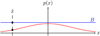 |
Fig. 1 Schematic illustration of rejection sampling. Given a continuous probability distribution function p(x) (solid red line) defined on some domain D ≡ [x−, x+], a single p-distributed sample |


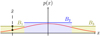 |
Fig. 2 Schematic illustration of bucketing. Rejection sampling as per Fig. 1 is inefficient if the upper bound B significantly overestimates the probability distribution function p(x), necessitating a large number of evaluations of p(x) per accepted sample. To increase efficiency, the domain D can be divided into disjoint subdomains D1,…,Dv (shaded with different colours), henceforth referred to as ‘buckets’. Then, separate upper bounds B1,…,Bv (solid coloured lines) can be estimated for the individual buckets. To sample a value |


3.2 Buckets
Rejection sampling is an efficient sampling scheme only if the upper bound λ+ is sufficiently close to the true interaction rate λ: the more the upper bound overestimates the interaction rate, the more sampled events have to be rejected, nevertheless each incurring an evaluation of the entity interaction rate function λent(q, q′, δ).
In order to increase the efficiency of rejection sampling, we introduce the ‘bucketing scheme’, the concept of which is explained schematically in Fig. 2. The basic idea is to group similar entities in ‘buckets’, then to compute upper bounds of the interaction rates between buckets of entities. To group entities in buckets, we first need a bucketing criterion, that is, a function B : ℚ → 𝕁 that maps a vector of entity properties q to an element B(q) in some discrete ordered set 𝕁. In simpler words, for any given entity j the function B(qj) tells which bucket this entity is in. Each bucket is uniquely identified by an element J ∈ ∈, henceforth referred to as the label of the bucket. A convenient choice for a label would be a d-dimensional vector of integers, ∈ ≡ ℤd, which can be ordered lexicographically.
With Bj we denote the label of the bucket which entity j is currently in, which we initialise as
 (36)
(36)
We refer to the set of entity indices associated with a bucket with label J ∈ ℤ as
 (37)
(37)
In other words, 𝔗J is the index set of entities that are in bucket J. The number of entities in a bucket is denoted
 (38)
(38)
consistent with n = #𝔗, where #S refers to the cardinality of some set S. Buckets are necessarily disjoint,
 (39)
(39)
meaning that each entity belongs to one, and only one, bucket. The set of occupied bucket labels, that is, the labels of the buckets which contain at least one entity, is
 (40)
(40)
the number of which is referred to as
 (41)
(41)
Because the bucketing scheme samples the space of bucket labels 𝕁 sparsely, the cost of storage and computational effort is a function of v.
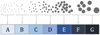 |
Fig. 3 Schematic illustration of the mass bucketing criterion in Eq. (42). The orbs represent particles of different mass, visually represented as surface area, which are grouped into seven buckets. |
3.3 Example: Representative particles with mass
Pursuing the example given in Sect. 2.6 further, we identify entities with representative particles. We also assume that each representative particle j has a mass mj = m(qj), and that the collision rate λ(qj, qk) is correlated with the masses mj and mk. The bucketing criterion is therefore chosen to be mass-dependent. A typical physical scenario studied with an RPMC coagulation simulation covers a dynamic range of several orders of magnitude in particle mass, hence a logarithmic dependency on mass is appropriate. A simple yet effective one-dimensional bucketing criterion thus is
 (42)
(42)
for some reference mass m0, where m(q) is the mass of a representative particle with properties q, and where the expression  denotes the floor function. The bucket density θm is a simulation parameter which specifies how many buckets per mass decade should be used, thus indirectly controlling the number of occupied buckets v. The bucketing criterion in Eq. (42) is visualised schematically in Fig. 3.
As explained in Sect. 2.6, for the extended RPMC method, particle–swarm interaction rates differ between the different interaction regimes (the many-particles regime and the few-particles regime). Therefore, it is reasonable to also use the swarm multiplicity as part of the bucketing criterion. Another change brought about by the extended RPMC method is that swarm masses are allowed to vary. In the original definition of the method, the same fraction of the total mass had been assigned to each swarm. The interaction rate λjk has a strong dependency on the number of particles represented, as seen in the (near-)proportionality to N(q′) in Eq. (16), and therefore also depends on the swarm mass to which the number of particles relates as N(q) = M(q)/m(q), where M(q) refers to the total mass represented by the swarm. For this reason, we also want to have the swarm mass be part of the bucketing criterion.
For the extended RPMC method we therefore propose the following three-dimensional bucketing criterion:
 (43)
(43)
with M0 = 𝓜/n the average swarm mass, 𝓜 the total mass of particles in the system, and the bucket density θM a simulation parameter specifying the number of buckets to use per decade of swarm masses. The classifier C(q) is defined as
 (44)
(44)
with Nth the particle regime threshold.
The traditional RPMC method always employs an equal-mass sampling, Mi = M0 ∀i ∈ 𝔗, which stays unaltered over the course of the simulation, and it entirely operates in the many-particles regime, Ni ≫ 1 ∀i ∈ 𝔗, and hence Ni > Nth ∀i ∈ 𝔗. Therefore, the first and second components of Eq. (43) would always evaluate to 1 and  , rendering this bucketing criterion equivalent to Eq. (42) in this case.
3.4 Sampling an event
Let us assume that, given a bucket J and its constituent entities j ∈ 𝔗J, we can compute its bucket properties, which we denote as QJ; and that, given two buckets J, K, and their associated bucket properties QJ, QK, we can compute an upper bound  for the interaction rates λjk between any entities j, k associated with these buckets,
 (45)
(45)
or equivalently
 (46)
(46)
Bucket properties and the computation of bucket-bucket interaction rate bounds remain unspecified here but are discussed in detail in Sect. 4.
We then define the upper bounds of the cumulative interaction rates for all buckets J,
 (47)
(47)
and the upper bound of the global interaction rate
 (48)
(48)
Inserting Eqs. (46) and (47) into Eq. (48) proves that λ+ indeed constitutes an upper bound to the global rate of interactions λ (Eq. (6)):
 (49)
(49)
Using the upper bounds λ+ and  , we can now implement the rejection sampling scheme of Sect. 3.1 more efficiently by interchanging the acceptance decision and the selection ofentity indices j, k:
1. First, we randomly choose bucket indices J, K with a probability
 (50)
(50)
2. using discrete inverse transform sampling as per Sect. 2.4.2. We then randomly choose entity indices j∈ 𝔗J, k ∈ 𝔗K with the probability
 (51)
(51)
3. which is independent of j and k, amounting to uniform or unweighted sampling. 3. Then we compute the interaction rate λjk of the entities chosen. The interaction event is then accepted with a probability of
 (52)
(52)
Combining all three probabilities, we obtain the selection probability
 (53)
(53)
which we find identical to the combined sampling probability Pjk in Eq. (35), thereby proving that this selection process is equivalent.
3.5 The bucketing algorithm
We now describe how a general compound Poisson process as defined in Sect. 2.2 can be simulated with the bucketing scheme. The proposed algorithm consists of the following steps:
- 1.
Initialise simulation.
- 1.i.
Distribute all entities j to buckets. To this end, for every entity j determine the entity bucket label Bj ← B(qj). Assemble a list of occupied buckets and, for every occupied bucket, a list of the entities in it.
- 1.ii.
For all occupied buckets J ∈ ∈, compute the bucket properties QJ, which are a function of the properties qj of the entities in the bucket, j ∈ 𝔗J.
- 1.iii.
For all pairs of buckets J, K ∈ 𝓑, compute bucket-bucket interaction rate upper bounds
 .
. - 1.iv.
Compute the upper bounds for the cumulative bucket interaction rate bound
 for all occupied buckets J ∈ 𝓑 by summation of
  , and compute the upper bound of the global interaction rate λ+ by summation of all
- 1.i.
- 2.
Sample an event.
- 2.i.
Sample an event interarrival time ∆t with Eq. (4) using λ+ as the interaction rate.
- 2.ii.
If the time exceeds the timescale of external updates, ∆t > T, apply the external updates, execute Step 3 for every entity whose properties underwent significant changes during the external update, then adjust ∆t, t, T as per Eqs. ((28)–(31)), then start over with Step 2.i.
- 2.iii.
It can be assumed henceforth that Δt ≤ T: The sampled tentative interaction event may occur within the external updating timescale. Thus, using discrete inverse transform sampling with the stored interaction rate bounds
 , randomly choose the buckets J, K ∈ 𝔅 which contain the entities possibly determined to undergo an interaction event.
 - 2.iv.
Using uniform sampling, randomly choose a pair of entities j ∈ 𝔗, k ∈ 𝔗K.
- 2.v.
Compute the interaction rate λjk. Accept the event with probability Paccept,jk (Eq. (52)).
Advance the system time by the event interarrival time, t ← t + Δt (Eq. (33)).
- 2.vi.
If the event was accepted, simulate the interaction between entities j and k, thereby possibly altering the entity properties
 and then execute Step 3 for all entities whose properties have changed (none, j, k, or both j and k).
 - 2.vii.
Continue with Step 2.i.
- 2.i.
- 3.
Subroutine: update a given entity j.
- 3.i.
Determine the old and new bucket labels J := Bj, J′ := B′j. Move the entity to the new bucket if J′ ≠ J.
- 3.ii.
For bucket J′, update (if necessary) or recompute (if due) the bucket properties QJ′.
Section 4.4 precisely defines what ‘updating’ means and how we decide whether updating suffices or the bucket properties need to be recomputed.
- 3.iii.
If the bucket properties were recomputed, or if the updating step caused an alteration of the bucket properties QJ′ of the new bucket J′, recompute the bucket-bucket interaction rate upper bounds
 for all occupied buckets K ∈ 𝔅.
 - 3.iv.
For all occupied buckets K ∈ 𝔅, update the cumulative interaction rate bounds
 incrementally to account for any changes to
  and recompute λ+ by summation of all
  .
.
- 3.i.
3.6 Data structures
The efficiency of the algorithm presented in Sect. 3.5 is bounded by the efficiency of its various mapping and enumeration steps. The data structures chosen to represent the simulation state are thus of critical importance.
In our reference implementation, we represent the simulation state with the following data structures:
An array (qj)j∈l of length n which holds the entity properties for all entities j ∈ 𝔗.
The upper bound for the total interaction rate λ+.
-
An array (DJ)J∈𝔅 of length v which for every occupied bucket J ∈ 𝔅 stores a tuple
 (54)
(54)holding the bucket label J, the bucket properties QJ, an array of entities 𝔗J, an array of bucket–bucket interaction data upper bounds
 , and the cumulative bucket interaction rate upper bound
  .
.The order of the entity indices in the 𝔗J arrays is arbitrary. The order of the (DJ)J∈𝔅 array is arbitrary as well but must coincide with the order of the arrays of bucket-bucket interaction data upper bounds
 for all J ∈ 𝔅.
 -
An array (J, bJ)J∈𝔅 of length v which for every occupied bucket J ∈ 𝔅 stores the index bJ of the corresponding element in the (DJ)J∈𝔅 array.
The array is ordered by J.
-
An array (Ej)j∈𝔗 of length n which for every entity j ∈ 𝔗 stores a tuple
 (55)
(55)holding the bucket labels Bj and the offsets oj at which the entity indices are stored in the array held by
 .
.
The relations between the arrays (DJ)J∈𝔅, (J, bJ)J∈𝔅, and (Ej)j∈𝔗 are exemplified in Fig. 4. With these data structures, the bucketing algorithm can be implemented very efficiently, as we shall explore in the next section.
Although a particular choice of data structures is discussed here, the bucketing algorithm could of course be implemented differently. For example, instead of storing an array of entries 𝔗J for every bucket J ∈ 𝔅, all entries could be stored in a single contiguous array ordered by bucket index, thereby reducing the amount of memory reallocations required while increasing the cost of moving entities between buckets and the cost of adding or removing buckets.
3.7 Cost model
In the following we estimate the memory requirement and the computational cost of simulating a compound Poisson process with the bucketing scheme when implemented with the choice of data structures described in Sect. 3.6.
The bucket properties QJ and the computation of upper bounds for bucket–bucket interaction rates are discussed in Sect. 4. For now, without specifying them any further, we only make two assumptions for the purpose of assessing the cost of the simulation. Firstly, given a bucket J ∈ 𝔅 holding nJ entities, we assume that the bucket properties QJ can be computed by traversal of the entity properties qj of all entities in the bucket j ∈ ?J, and therefore with nJ computational steps. Secondly, given the bucket properties QJ, QK for two buckets J, K ∈ 𝔅, we assume that an upper bound for the bucket–bucket interaction rate  can be computed in constant time, that is, with computational effort independent of the number of entities held by buckets J and K.
In the bucketing scheme, the same n vectors of entity properties qj as in the traditional sampling scheme need to be tracked, but in addition, only v2 upper bounds of bucket–bucket interaction rates as well as v elements of per-bucket data such as bucket properties and cumulative interaction rate upper bounds must be stored, amounting to an approximate memory requirement of
 (56)
(56)
floating-point values, where α = dim ℚ again is the number of floating-point values needed to represent the properties qj of some entity j, and β represents the number of floating-point values required to store the properties QJ of some bucket J.
In addition to the elementary computational costs defined in Sect. 2.8, we define the following additional costs specific to the bucketing scheme:
CQ, the cost of updating the set of bucket properties QJ for a given bucket J ∈ 𝔅 to account for an entity being added to or removed from the bucket;
 , the cost of computing an upper bound for the bucket-bucket interaction rate from two sets of bucket properties Q, Q′.
The proposed algorithm of the bucketing scheme employs dynamically sized data structures. The runtime cost and memory overhead of dynamic memory allocation is neglected in the following discussion.
To set up a simulation, we first traverse the list of entities j ∈ 𝔗, evaluate the bucketing criterion B(q) to determine the corresponding bucket label Bj ← B(qj) for every entity, store the label in the Ej array, and store the list of all bucket labels in the sorted array of tuples (J, bJ)J∈𝔅. This can be done with amortised (n + v log v) operations by accumulating and subsequently sorting occupied bucket labels. For every occupied bucket we allocate an entry in the DJ array which we refer to with the bJ index. We then iterate through the list of entities j ∈ 𝔗 a second time, look up the bucket labels Bj in the Ej array, locate the bucket in the (J, bJ) array with binary search, and append the entity to the bucket’s list of entity indices  , storing the entity index position in oj, which entails an average number of n log v steps. With every bucket having available a list of the entities in it, we can now iterate through the array of buckets and compute and store the bucket properties QJ for every bucket J ∈ 𝔅 at a total cost of ΣJ nJ CQ = nCQ. Finally, we iterate over all pairs of buckets J, K ∈ 𝔅 and compute and append the bucket–bucket interaction rate upper bounds
  to the array
  of bucket J, which has a cost of
  . With v2 arithmetic operations, we also compute the cumulative bucket interaction rate upper bounds
  and the total interaction rate upper bound λ+. The total cost of initialising the simulation thus amounts to
 (57)
(57)
Sampling an event candidate requires drawing one uniform random number for choosing an interarrival time, two random numbers and v additions on average for determining a pair of buckets, and another two random numbers for choosing entity indices. An event candidate can be accepted or rejected, which is decided by computing the interaction rate between the entities sampled to determine the acceptance probability (Eq. (52)) and by choosing whether to accept by drawing another random number. Let us assume that the average probability of acceptance is p ∈ (0,1]; then, for one event to be simulated, p−1 candidates have to be drawn on average, and the cost of sampling an event therefore is
 (58)
(58)
When the properties qj of an entity j are changed either by an interaction or by external events, the bucket properties QJ of the corresponding bucket J = Bj, all bucket–ucket interaction rate bounds involving bucket J, and all cumulative bucket interaction rate bounds need to be updated. Locating the bucket of entity j in the sorted array of tuples (J, bJ)J∈𝔅 with binary search requires log v comparisons on average, and updating the upper bound for the interaction rate λ+ requires recomputing and summing up an average number of v bucket–ucket interaction rate bounds, amounting to an approximated cost of
 (59)
(59)
Entities sometimes need to be moved to another bucket, and as a consequence, buckets sometimes need to be added and removed. With the data structures adopted for our reference implementation, either operation can be performed in amortised 𝒪(1) steps with a manoeuvre sketched in Fig. 5 which we refer to as ‘castling’ because of its vague resemblance of the eponymous chess move.
Following the reasoning in Sect. 2.8, we estimate the simulation cost rate as
 (60)
(60)
![Mathematical equation: $\eqalign{ & \approx \left( {{p^{ - 1}}nv} \right)\tilde \lambda {C_{{\rm{op}}}} \cr & \,\,\, + \left( {{p^{ - 1}}n} \right)\tilde \lambda \left( {6{C_{{\rm{rand }}}} + {C_\lambda }} \right) \cr & \,\,\, + (nv)\left[ {\tilde \lambda + {{\tilde \lambda }_{{\rm{ext }}}}} \right]\left( {{C_{{\lambda ^ + }}} + {C_{{\rm{op}}}}} \right) \cr & \,\,\, + n\left[ {\tilde \lambda \left( {{C_Q} + {C_{{\rm{action }}}}} \right) + {{\tilde \lambda }_{{\rm{ext }}}}{C_Q}} \right], \cr} $](/articles/aa/full_html/2024/04/aa47304-23/aa47304-23-eq97.png) (61)
(61)
where a (n log v) ![Mathematical equation: $\left[ {\tilde \lambda + {{\tilde \lambda }_{{\rm{ext}}}}} \right]{C_{{\rm{op}}}}$](/articles/aa/full_html/2024/04/aa47304-23/aa47304-23-eq98.png) term has been neglected.
term has been neglected.
The cost estimate is more complex than the estimate given for the traditional scheme in Eq. (26), but it is evident that no term scales with n2 or with n log n. However, we observe that, because buckets are allocated sparsely, there cannot be more occupied buckets than entities,
 (62)
(62)
and thus n v is an upper bound to v2: the cost rate of the bucketing scheme thus scales at least quadratically with the number of buckets, just as the cost rate of the traditional implementation scales quadratically with the number of entities.
The average probability of acceptance p quantifies the efficiency of the bucketing scheme. For an inefficient bucketing scheme, p is very small, and hence p−1 is large, allowing the first two terms in Eq. (61), which comprise the cost of rejection sampling, to dominate the simulation cost rate. Conversely, if the bucketing scheme is efficient, p, and thus p−1 as well, approaches unity, allowing the latter two terms in Eq. (61) to dominate. If we adjust the balance between rejection sampling and updating by refining or coarsening the bucketing scheme, or by making the bucketing scheme slightly hysteretic (cf. Sect. 4.5), then we can achieve better overall performance, as studied in Sect. 6.3.5.
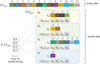 |
Fig. 4 Example illustrating the data structures used to implement the bucketing scheme as described in Sect. 3.6. This example comprises an ensemble of n = 13 entities partitioned in v = 4 buckets, with the bucket labels being designated as A, B, C, D, ordered lexicographically, and using 0-based numeric indices for all other indexing purposes. Entity indices are printed in normal type. The indices of the array entries at which the entity indices are stored in their associated buckets are printed in italic type. Element referral is indicated by dashed lines. Some elements of the DJ tuples were omitted in the visual representation. |
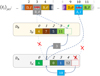 |
Fig. 5 Example demonstrating how to move an entity to a different bucket in 𝒪(1) steps. To move entity 4 from bucket A to bucket B, append an element to the list of entities in bucket B, and move the last entity in bucket A to the previous location of entity 4. Only two elements in the array (Ej)j∈𝔗 have to be updated. Element movement is symbolised with solid lines, and element referral is indicated by dashed lines. Addition and removal of entries to and from arrays is indicated with boxes of green and red colour, respectively. |
4 Computing interaction rate bounds
In our description of the bucketing algorithm in Sect. 3.5, two aspects had remained unspecified: the nature and purpose of the bucket properties QJ, and the computation of upper bounds for bucket-bucket interaction rates  from bucket properties QJ, QK of two buckets J, K ∈ 𝔅.
The definition of bucket-bucket interaction rate upper bounds given in Eq. (46) suggests that bounds could be computed as
 (63)
(63)
for two given buckets J, K ∈ 𝔅. Naïvely, this would require the evaluation of the entity–entity interaction rate λ jk for all pairs of entities j ∈ 𝔗J and k ∈ 𝔗K, and therefore nJ ⋅ nK evaluations of the entity interaction rate function λent(q, q′, δ). Because, for v occupied buckets, a total number of v2 bucket-bucket interaction rate upper bounds need to be computed, and because ΣJ nJ = n, this amounts to n2 evaluations of λent(q, q′, δ), which would be prohibitively expensive. But Eq. (63) can be evaluated much more efficiently, as we shall now demonstrate with an example.
4.1 Example: Linear kernel
The ‘linear kernel’
 (64)
(64)
with some constant λ0 leads to a special case of the Smoluchowski equation (Eq. (1)) for which the equation can be solved analytically (e.g. Ohtsuki et al. 1990), and which is hence often used to verify numerical methods for the simulation of coagulation processes. In a representative particle simulation where all swarms are many-particle swarms, Nk ≫ 1 ∀k ∈ 𝔗, the particle–swarm interaction rate λjk would then be
 (65)
(65)
as per Eq. (16). Inserting this expression into Eq. (63), we find that a bucket–bucket interaction rate bound can be computed as a function of bucket-specific upper bounds,
![Mathematical equation: $\eqalign{& \lambda _{JK}^ + \leftarrow \mathop {\max }\limits_{j \in {I_J},k \in {I_K}} {\lambda _0}\left( {{N_k}{m_j} + {M_k}} \right) \cr & \,\,\,\,\,\,\,\,\,\,\matrix{ { = {\lambda _0}\left[ {\mathop {\max }\limits_{k \in {I_K}} {N_k}\mathop {\max }\limits_{j \in {I_J}} {m_j} + {M \over n}} \right]} \hfill \cr { = {\lambda _0}\left[ {N_K^ + m_J^ + + {M \over n}} \right],} \hfill \cr } \cr} $](/articles/aa/full_html/2024/04/aa47304-23/aa47304-23-eq104.png) (66)
(66)
where we used the swarm mass Mk = Nkmk, assumed an equal-mass sampling where every swarm holds the same fraction of the total mass ℳ,
 (67)
(67)
and where the notation
 (68)
(68)
refers to the bucket-specific lower and upper bounds  of some property xk for entities k in a bucket K. Computing a bucket-specific upper bound only requires traversal of all entities in the bucket, and hence nJ operations for a bucket J, or n operations for all buckets. In the case of the linear kernel, we could therefore define the bucket properties as a tuple
 (69)
(69)
which for any bucket J can be computed with nJ operations. Subsequently, given the bucket properties QJ, QK of two buckets J and K, a bucket–bucket interaction rate upper bound  can be computed directly as per Eq. (66), thereby meeting the complexity requirements stated in Sect. 3.7. We note that the upper bound given by Eq. (66) is optimal: it is an exact upper bound on the particle–swarm interaction rates λjk for j ∈ 𝔗J, k ∈ 𝔗K, or in other words, no better bound exists. This quality is difficult to retain except in the simplest of cases.
Results for an RPMC simulation of coagulation with the linear kernel using the bucketing scheme are shown in Fig. 6. The analytical solution is given as a reference.
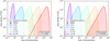 |
Fig. 6 Analytical solutions and RPMC simulations for the coagulation test with the linear kernel (Eq. (64)) using the bucketing scheme. The RPMC simulation runs use n = 1024 and n = 65 536 representative particles, respectively. |
4.2 Example: Runaway kernel
As another example, we consider the runaway kernel, a test kernel modelled after the gravitational focussing effect (cf. e.g. Armitage 2007, Sect. III.B.l) which was introduced in the companion paper Beutel & Dullemond (2023, Sect. 6.2) for the purpose of studying the swarm regime transition:
![Mathematical equation: $\lambda \left( {m,{m^\prime }} \right) = {\lambda _0}\max {\left( {m,{m^\prime }} \right)^{2/3}}\left[ {1 + {{\left( {{{\max \left( {m,{m^\prime }} \right)} \over {{m_{{\rm{th }}}}}}} \right)}^{2/3}}} \right],$](/articles/aa/full_html/2024/04/aa47304-23/aa47304-23-eq110.png) (70)
(70)
where λ0 is some constant and is a threshold mass.
As with the linear kernel, an upper bound of the bucket–bucket interaction rate can be given in terms of bucket-specific bounds,
![Mathematical equation: $\lambda _{JK}^ + \leftarrow {\lambda _0}N_K^ + {\left( {m_{J,K}^ + } \right)^{2/3}}\left[ {1 + {{\left( {{{m_{J,K}^ + } \over {{m_{{\rm{th}}}}}}} \right)}^{2/3}}} \right],$](/articles/aa/full_html/2024/04/aa47304-23/aa47304-23-eq111.png) (71)
(71)
where we used the abbreviation  , the sub-multiplicativity of the maximum norm,
 (72)
(72)
for sequences of positive semi-definite quantities (ai)i, (bi)i, and the monotonicity of exponentiation. Although this upper bound is no longer exact2, it can be obtained directly from bucket properties
 (73)
(73)
and thus also meets the complexity requirements stated in Sect. 3.7.
Results for an RPMC simulation of coagulation with the runaway kernel using the bucketing scheme are shown in Fig. 7. The runaway kernel is shown in Fig. 8 along with the emerging entity interaction rate λent(q,q′,δ). For comparison, two snapshots from the RPMC simulation are given in Fig. 9. In both figures, a discontinuity can be observed as swarms Nk are split up once their swarm particle count Nk no longer exceeds the particle regime threshold Nth. Self-representing particles, that is, representative particles k with a swarm particle count of Nk = 1, cannot interact with their own swarm, hence their self-interaction rate is λkk = 0, as seen in the lower left panel of Fig. 9. Indices are grouped by buckets, and the corresponding bucket–bucket interaction rate bounds  are shown in the right panels of Fig. 9.
4.3 General interaction rate bounds
We demonstrated how to efficiently compute upper bounds for the bucket–bucket interaction rates for the examples given in Sects. 4.1 and 4.2 by defining a set of bucket-specific upper bounds as bucket properties, inserting the respective interaction rate function into Eq. (63), and rewriting the upper-bound estimate as a function of the bucket properties. The generalisation of this approach leads to the concept of interval arithmetic, which is briefly introduced in Appendix A along with interval notation such as [x] = [x−, x+] and the Fundamental Theorem of Interval Arithmetic. For a more thorough introduction to interval arithmetic, refer to Hickey et al. (2001); Moore et al. (2009); Alefeld & Herzberger (2012).
By virtue of the Fundamental Theorem of Interval Arithmetic, we can obtain an interval extension of the linear kernel (Eq. (64)),
![Mathematical equation: $\Lambda \left( {[m],\left[ {{m^\prime }} \right]} \right) = {\lambda _0} \cdot \left( {[m] + \left[ {{m^\prime }} \right]} \right),$](/articles/aa/full_html/2024/04/aa47304-23/aa47304-23-eq116.png) (74)
(74)
and likewise of the runaway kernel (Eq. (70)),
![Mathematical equation: $\eqalign{ & \Lambda \left( {[m],\left[ {{m^\prime }} \right]} \right) = {\lambda _0} \cdot {\left( {{\mathop{\rm Max}\nolimits} \left( {[m],\left[ {{m^\prime }} \right]} \right)} \right)^{2/3}} \cr & \,\,\,\,\,\,\,\,\,\,\,\,\,\,\,\,\,\,\,\,\,\,\,\,\,\,\,\,\,\,\, \times \left[ {1 + {{\left( {{{{\mathop{\rm Max}\nolimits} \left( {[m],\left[ {{m^\prime }} \right]} \right)} \over {{m_{{\rm{th }}}}}}} \right)}^{2/3}}} \right], \cr} $](/articles/aa/full_html/2024/04/aa47304-23/aa47304-23-eq117.png) (75)
(75)
where the exact interval extension of the max function is given by
![Mathematical equation: ${\mathop{\rm Max}\nolimits} ([x],[y]) = \left[ {\max \left( {{x^ - },{y^ - }} \right),\max \left( {{x^ + },{y^ + }} \right)} \right].$](/articles/aa/full_html/2024/04/aa47304-23/aa47304-23-eq118.png) (76)
(76)
Likewise, for the RPMC method with any raw collision rate function λ(q, q′) with an interval extension Λ([q], [q′]), an interval extension of the entity interaction rate function λent(q, q′,δ) in Eq. (16) can be obtained as
![Mathematical equation: ${\Lambda _{{\rm{ent}}}}\left( {[{\bf{q}}],\left[ {{{\bf{q}}^\prime }} \right],\Delta } \right): = {N^{{\rm{eff}}}}\left( {[{\bf{q}}],\left[ {{{\bf{q}}^\prime }} \right],\Delta } \right)\Lambda \left( {[{\bf{q}}],\left[ {{{\bf{q}}^\prime }} \right]} \right),$](/articles/aa/full_html/2024/04/aa47304-23/aa47304-23-eq119.png) (77)
(77)
where [q] denotes a vector of intervals, and where Δ ⊆ {0,1}, Δ ≠ 0 is a set containing 1 if the interaction can be an entity self-interaction and 0 if the interaction can be an interaction between different entities (and may thus contain both 0 and 1). Equivalently, we might state
![Mathematical equation: $\left[ {{\lambda _{JK}}} \right] = \left[ {N_{JK}^{{\rm{eff}}}} \right]\Lambda \left( {\left[ {{{\bf{q}}_J}} \right],\left[ {{{\bf{q}}_K}} \right]} \right),$](/articles/aa/full_html/2024/04/aa47304-23/aa47304-23-eq120.png) (78)
(78)
where we abbreviate the effective swarm particle count and its interval extension as
 (79)
(79)
![Mathematical equation: $\left[ {N_{JK}^{{\rm{eff}}}} \right]: = {N^{{\rm{eff}}}}\left( {\left[ {{{\bf{q}}_J}} \right],\left[ {{{\bf{q}}_K}} \right],{\Delta _{JK}}} \right),$](/articles/aa/full_html/2024/04/aa47304-23/aa47304-23-eq122.png) (80)
(80)
and where the set-valued self-interaction indicator ΔJK, the set extension of δjk, is given by
 (81)
(81)
in accordance with the definition of Δ given above: considering that we know only the buckets J, K which hold the interacting entities, we know that the interaction cannot be an entity self-interaction if the interacting entities are in different buckets, and that it is necessarily an entity self-interaction if both are in the same bucket and if that bucket only holds one entity. Otherwise, both self-interaction and non-self-interaction are possible.
In Beutel & Dullemond (2023), the notion of ‘boosting’ was introduced as a means of grouping together multiple similar events, and the boosted interaction rate was defined as
 (82)
(82)
where βjk, indicating the number of events grouped together, is the boost factor for an interaction of representative particle j with swarm k, and with the boosted swarm multiplicity factor  defined as
 (83)
(83)
with the boosted swarm particle count Njk = Nk/βjk and the effective swarm particle count correction factor  . A large value of βjk counteracts a large number of swarm particles Nk, and hence an interval extension of λjk can be obtained using the algebraically favourable rendering of Eq. (83),
![Mathematical equation: $\left[ {{\lambda _{JK}}} \right]: = \left[ {{N_{JK}}} \right] \cdot \left[ {V_{JK}^{{\rm{eff}}}} \right] \cdot \Lambda \left( {\left[ {{{\bf{q}}_J}} \right],\left[ {{{\bf{q}}_K}} \right]} \right).$](/articles/aa/full_html/2024/04/aa47304-23/aa47304-23-eq129.png) (84)
(84)
Here, the interval extensions of [NJK] and ![Mathematical equation: $\left[ {V_{JK}^{{\rm{eff}}}} \right]$](/articles/aa/full_html/2024/04/aa47304-23/aa47304-23-eq130.png) are obtained by composition as per the Fundamental Theorem of Interval Arithmetic, following the paradigm proposed by Beutel & Strzodka (2023) to obtain interval extensions of piecewise-defined functions such as Neff(q, q′, δ).
are obtained by composition as per the Fundamental Theorem of Interval Arithmetic, following the paradigm proposed by Beutel & Strzodka (2023) to obtain interval extensions of piecewise-defined functions such as Neff(q, q′, δ).
We thus define the bucket properties QJ for a bucket J as a vector of intervals of property bounds,
![Mathematical equation: ${Q_J}: = \left[ {{{\bf{q}}_J}} \right].$](/articles/aa/full_html/2024/04/aa47304-23/aa47304-23-eq131.png) (85)
(85)
We note, however, that it may be useful, and allow for tighter results in the interval extension of the interaction rate function, if we augment QJ with intervals of bounds of additional derived properties, as done in Eq. (69) for the linear kernel where we had defined the bucket properties QJ to include bounds for the particle property mj as well as the derived property Nj = (M/n)/mj.
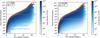 |
Fig. 7 RPMC simulations for the coagulation test with the runaway kernel (Eq. (70)) using the bucketing scheme. The RPMC simulation runs use n = 2048 and n = 65 536 representative particles, respectively, and a particle regime threshold of Nth = 10. The dimensionless threshold mass of mth = 107, marking the point where runaway growth ensues, is indicated by the dotted red horizontal lines, and the dashed orange lines indicates the representative particle mass M/(nNth) at which swarms are split up into individual particles. The plots show time series of histograms of the mass-weighted particle number density with bin counts colour-encoded on a logarithmic scale. The runaway particle is shown separately (red curve). Results have been averaged over 10 runs; the shaded surroundings of the red curve indicate the error bounds of the runaway particle mass. |
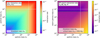 |
Fig. 8 Raw interaction rate λ(q, q′) and entity interaction rate λent(q, q′, δ) for the runaway kernel (Eq. (70)). Parameters are: λ0 = 10−10, threshold mass mth = 107, total mass ℳ = 1011, n = 2048 representative particles, particle regime threshold Nth = 10. Many-particles swarms (N(q) > Nth) are assumed to have homogeneous swarm mass M(q) = ℳ/n, whereas few-particles swarms (N(q) ≤ Nth) are assumed to have been split up to represent only themselves, N(q) = 1, and thus have swarm mass M(q) = m(q); hence the discontinuity at mcrit. |
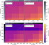 |
Fig. 9 Snapshots of the entity interaction rates λjk and corresponding bucket-bucket interaction rate bounds |

4.4 Updating bucket properties
We computed and stored an initial set of bucket property bounds QJ = [qJ] for all occupied buckets J ∈ 𝔅 as the Cartesian product of element–wise intervals
![Mathematical equation: $\left[ {{{\bf{q}}_J}} \right] \equiv \left[ {{q_{J,1}}} \right] \times \cdots \times \left[ {{q_{J,d}}} \right],$](/articles/aa/full_html/2024/04/aa47304-23/aa47304-23-eq132.png) (86)
(86)
![Mathematical equation: $\left[ {{q_{J,s}}} \right] \equiv \left[ {q_{J,s}^ - ,q_{J,s}^ + } \right] \leftarrow \left[ {\mathop {\min }\limits_{j \in {I_J}} {q_{j,s}},\mathop {\max }\limits_{j \in {I_J}} {q_{j,s}}} \right],$](/articles/aa/full_html/2024/04/aa47304-23/aa47304-23-eq133.png) (87)
(87)
where s denotes the component index of the d-dimensional property vector q. We sometimes abuse notation by employing the quantity itself as a placeholder for its index or its component, for instance writing qj,m instead of and use the component and the quantity interchangeably, mj = m(qj) = qj,m. For example, if entity properties consisted of a mass m and a charge c, the property vector would be qj = (mj, Cj); index s = m would refer to the mass dimension and index s ≡ c would refer to the charge dimension.
During simulation, an interaction between entities j and k usually changes some of their properties qj, qk. When the properties of an entity j change, the bucket property bounds [qJ], [qJ′] of the entity’s old and new buckets J and J′ (which may be identical) may also change. This is not always the case, though. As an example, consider a bucket with label A which contains three particles with masses m1 = 1 g, m2 = 3 g, and m3 = 7g. Presume that particle 2 suffers an interaction that grows its mass to  . Then the bucket property bounds for bucket A does not change; the minimum and maximum mass of any particle in the bucket are still 1 g and 7 g. In this case, the interaction rate bounds, which are a function of the bucket property bounds (Eq. (77) in the case of the RPMC method), do not change either and thus need not be recomputed in Step 3.iii, and no updates need to be performed in Step 3.iv of the bucketing algorithm.
Now let us instead assume that particle 3 undergoes a collision and grows to mass  . If the bucketing criterion B(q) still places particle 3 in the same bucket A, its bucket property bounds have to expand given that the maximum particle mass in the bucket is now 12 g; subsequently, the bucket interaction rate bounds for bucket A need to be recomputed in Step 3.iii, and the cumulative bucket interaction rate bounds need to be updated in Step 3.iv. Expanding the bucket property bounds is an operation with constant complexity, entailing only a min and max function call per bucket property, and thus is of negligible cost compared to the subsequent recomputation of interaction rate bounds and updating of cumulative interaction rate bounds.
Let us consider a third example: particle 3 still grows to  but the bucketing criterion B(q) now places it in a different bucket with label B. Let the bucket mass bounds of bucket B be [mB] = [11 g, 18 g]. The bucket property bounds of bucket B thus do not change, and no interaction rate bounds need to be recomputed in Step 3.iii. However, the number of entities nA and nB in buckets A and B have changed, and therefore in Step 3.iv the cumulative bucket interaction rate bounds must be updated.
So far we only described the expansion of bucket property bounds. It is possible that the bounds [qJ] currently stored for a bucket J are wider than necessary for the particles remaining in the bucket. In the third example considered above, this is the case for bucket A after particle 3 has been relocated to bucket B. Excessive property bounds lead to excessive interaction rate bounds and thus to an unnecessarily high rejection rate in the sampling step. We therefore strive to keep bucket property bounds tight. But while we could always recompute the bounds of a bucket J to keep them as tight as possible, this would come at a cost of nJ operations because all entities in the bucket would need to be processed. We therefore defer this recomputation by counting the number of times an entity in bucket J has changed since the last recomputation of bounds. Once the number exceeds the number of entities in the bucket nJ times the number of occupied buckets v, the bucket property bounds [qJ] are recomputed as per Eqs. (86) and (87). This recomputation then occurs every nJ ⋅ v updates at most, and thus has constant amortised computational cost per update. We also recompute the bounds if the number of rejected events exceeds a certain threshold such as n and if particles have been added to or removed from the bucket since the last recomputation. This recomputation also has constant amortised computational cost per simulated event.
4.5 Widening
If a simulation has to process a large number of events which only cause very slight changes to entity properties, it may spend a disproportionate fraction of its time updating bucket-bucket interaction rate bounds. In such a situation, it may be beneficial to choose slightly wider bucket bounds, which we refer to as ‘widening’. To widen a bucket means that, whenever a bucket’s property bounds are recomputed, its bounds are extended a little beyond the minimum and maximum property values of all entities in the bucket. So, instead of initialising the bucket property bounds with the minimum and maximum as per Eq. (87), they are widened as
![Mathematical equation: $\left[ {{q_{J,s}}} \right] \leftarrow \left[ {w_s^ - \left( {\mathop {\min \,}\limits_{j \in {I_J}} {q_{j,s}}} \right),w_s^ + \left( {\mathop {\max }\limits_{j \in {I_J}} \,{q_{j,s}}} \right)} \right],$](/articles/aa/full_html/2024/04/aa47304-23/aa47304-23-eq137.png) (88)
(88)
where s again denotes a component (e.g. mass, charge) of the vector of properties q. How property s is to be widened can be specified by the user-supplied widening functions  and
and  . The widening strategy should align with the bucketing criterion; for example, if a property such as mass is used for logarithmic bucketing as in Eqs. (42) and (43), it is best widened multiplicatively:
 (89)
(89)
where f ∈ [0, 1) is a simulation parameter indicating by which fraction of their width buckets should overlap. Conversely, a property used as a linear bucketing criterion would best be widened additively. For example, for a linear bucketing criterion such as
 (90)
(90)
where δx is a characteristic length and θx is the simulation parameter controlling the bucket width, a suitable widening function would be
 (91)
(91)
With widening, bucket property bounds exceed the strict bounds of the property values of their entities. This usually leads to overlapping buckets, and hence to a hysteresis effect in the bucket assignment of entities; with widening, an entity j may still reside in a bucket Bj different from the bucket it would be assigned to if the bucketing criterion B(qj) was re-evaluated with its current properties qj. Therefore, the likelihood is increased that a particle can remain in the same bucket after its properties undergo minuscule changes; bucket property bounds need to be updated (that is, extended or recomputed) less often, and the subsequent recomputations of bucket–bucket interaction rate bounds in Step 3.iii of the bucketing algorithm are avoided, all at the expense of a higher likelihood of rejection. The widening parameter f can thus be used to balance the sampling and the updating parts of the simulation. The impact of this parameter is studied experimentally in Sect. 6.3.5.
4.6 Efficiency and correctness
As observed in Sect. 4.1, it is usually not possible to estimate exact bounds if the interaction rate function is non-trivial. This does not constitute a problem – the bucketing scheme only requires an upper bound, not necessarily an exact one – but can negatively impact performance. By overestimating the bucket–bucket interaction rate, the acceptance probability in Eq. (52) decreases, and as a result we have to sample a larger number of potential events which are ultimately rejected. For optimal sampling performance, we thus desire a tight estimate of the bucket–bucket interaction rate upper bound. In a simulation which entails a large number of events bringing about only minute changes, some sampling performance may be traded for fewer updates, as proposed in Sect. 4.5, by widening the bucket property bounds by some fraction.
Regardless of whether a bound is exact or inexact, the fraction of rejected events is high if the entity–entity interaction rates λjk between entities in two given buckets J, K span many orders of magnitude. The computational cost of the simulation therefore depends on a suitable definition of the bucketing criterion B(q), chosen such that the interaction rates λjk between entities in any two buckets are of similar magnitude, and on a carefully crafted interval extension of the interaction kernel which avoids excess in the computation of bounds.
The bucketing criterion indirectly controls the number of occupied buckets v, and the simulation cost scales linearly with v according to Eq. (61). The bucketing criterion thus must find a compromise between a small number of buckets and a high rate of acceptance. With an inefficient bucketing criterion, the bucketing scheme can still be prohibitively expensive compared to the traditional inverse transform sampling scheme. But even with a suitable bucketing criterion, the traditional scheme may outperform the bucketing scheme for small numbers of entities n.
We conclude this section by again emphasising that the correctness of the scheme is in no way affected by the choice of a bucketing criterion or by the chosen upper bound estimate for the interaction rate. The bucketing scheme is statistically equivalent to the traditional sampling scheme; it does not impose additional physical or statistical requirements and does not introduce new approximations. The results of a simulation conducted with the bucketing scheme thus statistically match the results obtained with a traditional computational scheme; the simulation may only execute faster if an efficient bucketing criterion was chosen and if the upper bound estimates are not excessive. The correctness of the results is verified explicitly in Sect. 4.1, where the simulation result is compared to an analytical solution in Fig. 6. We also emphasise that the bucketing scheme had been used to run all simulations conducted in the companion paper (Beutel & Dullemond 2023), of which many had been compared to analytical solutions as well.
5 Locality
In simple geometric interaction models such as Eq. (13), the particle distribution is assumed to be homogeneous and isotropic. Often, however, a physical system features spatial inhomogeneities. For example, in a protoplanetary disk, the gas and dust density distribution may exhibit radial features such as rings, an amassment of dust grains, and cavities, a radial zone with little or no material (e.g. Huang et al. 2018).
To resolve spatial features in a stochastic simulation, we first augment the vector of entity properties qj with one or more components representing the location of the entity. In this section, we shall assume that the location of an entity j is represented by a one-dimensional quantity, noting that our approach can be generalised to higher dimensionality.
5.1 Local bucketing criteria
Typically, discrete interactions between entities are modelled as having a maximal spatial distance up to which interactions are possible. For example, two bodies j and k can collide only if their distance at their closest approach, represented by the impact parameter b, is not greater than their interaction radius Rcoll,
 (92)
(92)
which for massless spherical bodies is the sum of their bulk radii Rj and Rk,
 (93)
(93)
If the bodies are massive, collisions are possible at impact parameters greater than Rj + Rk because the mutual gravitational attraction boosts the effective collision cross-section, an effect known as gravitational focussing (e.g. Armitage 2007, Sect. III.B.1):
 (94)
(94)
where ![Mathematical equation: ${\rm{\Theta }} = 2G\left( {{m_j} + {m_k}} \right)/\left[ {\left( {{R_j} + {R_k}} \right)v_{\rm{a}}^2} \right]$](/articles/aa/full_html/2024/04/aa47304-23/aa47304-23-eq146.png) is the Safronov number (e.g. Weidenschilling 1989) with G the gravitational constant and va the approach velocity, the relative velocity at infinite distance. Assuming both bodies have circular planar orbits around the same central object, a lower bound for the impact parameter can be obtained as the difference of their semimajor axes,
is the Safronov number (e.g. Weidenschilling 1989) with G the gravitational constant and va the approach velocity, the relative velocity at infinite distance. Assuming both bodies have circular planar orbits around the same central object, a lower bound for the impact parameter can be obtained as the difference of their semimajor axes,
 (95)
(95)
If the orbit of a body is eccentric, its apsides (the points nearest to and farthest from the central object) have an orbital distance of a (1 − e) and a (1 + e), respectively, where a and e are the semimajor axis and the eccentricity of the orbit. Therefore, for two entities j, k with eccentric orbits, the interaction radius is enhanced further,
 (96)
(96)
It is clear that, if the lower bound for the impact parameter between two entities exceeds their maximal interaction distance, they cannot possibly interact. The raw interaction rate function λ(qj, qk) must take this into account and evaluate to 0 if the entities j, k are not in reach, implying that λjk = 0 in this case. But this does not hold true for the interval extension Λ([qJ], [qK]) if a non-local bucketing criterion is used which places entities with similar intrinsic properties in the same bucket regardless of their orbital position. For example, with the mass bucketing criterion of Eq. (42), the interactions between buckets J and K contribute a term  to the upper bound of the global interaction rate λ+ (Eq. (48)), implying that every entity in bucket J could possibly interact with any entity in bucket K with a maximal interaction rate of
  . In reality, the number of entity pairs from buckets J and K which could possibly interact may be much smaller than nJnK simply because many entity pairs would be out of reach. A non-local bucketing criterion therefore results in an excessive rejection rate, as events for out-of-reach entity pairs (j, k) are generated and must be rejected individually by evaluating λ(qj , qk).
An obvious remedy would be to use a local bucketing criterion instead. A local variant of the mass bucketing criterion given in Eq. (42) might additionally use the location aj ≡ a(qj) as a criterion for bucket labelling,
 (97)
(97)
where a0 is some reference location, and where δa is the spatial width of a bucket. If the interval extension Λ([qJ], [qK]) of the raw interaction rate is crafted with sufficient care, it evaluates to 0 if the entities in the two buckets J and K are always out of reach.
Although this approach is valid, it is not very practical. First, it is not clear how δa should be chosen. Let the interaction radius of two entities j, k be given by a function
 (98)
(98)
We could then set the smallest occurrent interaction radius as δa,
 (99)
(99)
In a representative particle method, we usually have to impose a lower limit Rjk ≥ Rmin, where the simulation parameter Rmin represents the smallest length to be resolved by the simulation, because of the finite number of representative entities. This gives rise to a good approximation for Eq. (99),
 (100)
(100)
We note that this choice of δa would grow the number of occupied buckets v dramatically. Even worse: as the number of representative particles n is increased, we are able to afford a better resolution; but shrinking Rmin, and thus δa, then grows the number of occupied buckets v even further. As we had found in Sect. 3.7, the cost of the simulation strongly depends on the total number of occupied buckets v: the memory requirements (Eq. (56)) scale with v2, and the simulation cost rate (Eq. (61)) scales with n⋅v in the dominant terms. Even though the number of out-of-reach rejections can be greatly reduced with a local bucketing criterion, it is questionable whether this outweighs the cost of updating all the additional buckets.
5.2 Local sub-buckets
We would like to retain the benefit of a local bucketing criterion – elimination of most out-of-reach rejections – without having to pay for an exploding number of buckets. This desire gives rise to the notion of spatial sub-bucketing. The basic idea is that the entities in a given bucket are grouped in sub-buckets according to their location. Interaction rate bounds are computed for bucket-bucket pairings as before, but when computing an upper bound of the global interaction rate λ, the sub-buckets are used to estimate a maximal number of entity pairs  from buckets J and K which could possibly interact, resulting in a better bound of the global interaction rate λ,
 (101)
(101)
 (102)
(102)
cf. Eqs. (47) and (48). Ideally,  , and thus
  .
.
Let an entity j be associated with a dimensionless location lj ≡ l(qj). Given a sub-bucket s of bucket J and a second bucket K, we need an efficient means of locating and enumerating the sub-buckets t in bucket K which are in reach of sub-bucket s. A sub-bucket t is considered ‘in reach’ if any of the entities it might hold could possibly interact with any entity possibly in s. For reasons that become apparent as this predicate is specified more precisely, the rounding behaviour of floatingpoint arithmetic makes it unsuitable for determining the range of reachable sub-buckets; we therefore opt to employ integer arithmetic instead. Sub-bucket widths therefore need to be granular, that is, multiples of some common length scale. This length scale is represented as unity in the dimensionless location l; on this dimensionless scale, the width of a sub-bucket is always a positive integer, a multiple of 1.
Location l can be defined according to the nature of the spatial coordinate. For example, the location of a representative body on some circumstellar orbit could be defined in terms of its semimajor axis a as
 (103)
(103)
where the integer-valued simulation parameter dmin > 0 is a granularity measure, a0 is some reference position, and Rmin is the minimal resolved length scale. lj· ≡ l(qj) then represents the location of entity j relative to the reference position a0 in units of (Rmin/wmin).
In accordance with the definition of location l(q), the sub-bucketing scheme requires a function
 (104)
(104)
which quantifies the interaction distance between entities j and k, and its interval extension
![Mathematical equation: $\left[ {{d_{JK}}} \right] = D\left( {\left[ {{{\bf{q}}_J}} \right],\left[ {{{\bf{q}}_K}} \right]} \right).$](/articles/aa/full_html/2024/04/aa47304-23/aa47304-23-eq162.png) (105)
(105)
A dimensionless equivalent of the interaction radius introduced in Sect. 5.1, the interaction distance is defined as the greatest location distance at which two entities with entity properties q and q′ could possibly interact,
 (106)
(106)
For a location defined as a linear function of the semimajor axis as in Eq. (103), the interaction distance is given in terms of the interaction radius (Eq. (98)) as
 (107)
(107)
Other definitions of location and distance are possible as long as the domain of locations is a one-dimensional metric space with a Euclidean distance measure. For example, if interaction radii tend to scale with the position, Rjj ∝ aj, then a logarithmic definition would be more appropriate. Such a definition is elaborated in Appendix B.
After entities have been grouped into buckets, the width of the sub-buckets in a bucket J is chosen as
 (108)
(108)
With the linear definition of location and distance in Eqs. (103) and (107), imposing dmin as a lower bound ensures that a sub-bucket cannot be narrower than the minimum resolved length scale. The bucket self-interaction distance is a reasonable compromise for bucket size because, in most physical models, interaction radii are of vaguely additive nature,
 (109)
(109)
Given an entity j in bucket J, the sub-bucket index sj ≡ sJ (lj) of j is then defined as
 (110)
(110)
For every bucket, the simulation maintains a dynamic array of records indexed with s, where every record stores a dynamic array of entity indices in that sub-bucket. As before, entities can be moved between buckets and sub-buckets with constant complexity using the ‘castling’ manoeuvre (cf. Fig. 5).
5.3 Sub-bucket reach
By inverting Eq. (110), we find the range of entity locations associated with a given sub-bucket index s to be the interval-valued function
 (111)
(111)
A sub-bucket s from bucket J and a sub-bucket t from bucket K shall be called ‘in reach’ of each other if an entity that would be grouped in sub-bucket s could possibly be within the rounded interaction distance bound ![Mathematical equation: $\left[ {d_{JK}^ + } \right]$](/articles/aa/full_html/2024/04/aa47304-23/aa47304-23-eq169.png) of any entity that would belong in sub-bucket t, as visualised in Fig. 10. Given a sub-bucket s in a bucket j, we can thus combine Eqs. (110) and (111) to obtain the interval of sub-bucket indices UK,J(s) in bucket K which are in reach of s:
of any entity that would belong in sub-bucket t, as visualised in Fig. 10. Given a sub-bucket s in a bucket j, we can thus combine Eqs. (110) and (111) to obtain the interval of sub-bucket indices UK,J(s) in bucket K which are in reach of s:
 (112)
(112)
where the ‘±’ is sloppy interval notation,
 (113)
(113)
and where SK([l]) is the interval extension of sK(l),
![Mathematical equation: ${S_K}([l]) = \left\lfloor {{{[l]} \over {{w_K}}} + {1 \over 2}} \right\rfloor .$](/articles/aa/full_html/2024/04/aa47304-23/aa47304-23-eq172.png) (114)
(114)
Using the identity
![Mathematical equation: $\left\lfloor {[a,b)} \right\rfloor = [\left\lfloor a \right\rfloor ,\left\lceil {b - 1} \right\rceil ]$](/articles/aa/full_html/2024/04/aa47304-23/aa47304-23-eq173.png) (115)
(115)
we insert definitions into Eq. (112) to find a ≠ b
![Mathematical equation: $\eqalign{ & {U_{K,J}}(s) = \left[ {\left\lfloor {{{{w_J}(2s - 1) - \left( {2\left\lceil {d_{JK}^ + } \right\rceil - {w_K}} \right)} \over {2{w_K}}}} \right\rfloor ,} \right. \cr & \,\,\,\,\,\,\,\,\,\,\,\,\,\,\,\,\,\,\,\,\,\left. {\left\lceil {{{{w_J}(2s + 1) + \left( {2\left\lceil {d_{JK}^ + } \right\rceil - {w_K}} \right)} \over {2{w_K}}}} \right\rceil } \right]{\rm{.}} \cr} $](/articles/aa/full_html/2024/04/aa47304-23/aa47304-23-eq175.png) (116)
(116)
According to Eq. (108), wj and wK are integers, and therefore both interval bounds in Eq. (116) are fractions of integers. To understand why this is significant, let us pretend that the unrounded interaction distance bound  , ratherthan
 ![Mathematical equation: $\left[ {d_{JK}^ + } \right]$](/articles/aa/full_html/2024/04/aa47304-23/aa47304-23-eq177.png) , had been used to define the notion of being ‘in reach’ in Eq. (112) and the sub-bucket width in Eq. (108). Floating-point additions, multiplications, and divisions are subject to rounding error, which can lead to significant differences in UK,J (s) if the value of the fractions in Eq. (116) is close to an integer. We note that being ‘in reach’ is a commutative relation,
, had been used to define the notion of being ‘in reach’ in Eq. (112) and the sub-bucket width in Eq. (108). Floating-point additions, multiplications, and divisions are subject to rounding error, which can lead to significant differences in UK,J (s) if the value of the fractions in Eq. (116) is close to an integer. We note that being ‘in reach’ is a commutative relation,
 (117)
(117)
However, due to different accumulation of rounding errors in the different algebraic computations of UK,J(s) and UJ,K(t), a sub-bucket t from bucket K might be deemed in reach of a sub-bucket s from bucket J, while at the same time s would not be considered in reach of t. In the incremental updating approach explained in the subsequent Sect. 5.4, this would violate consistency. Conversely, if both numerators and denominators in Eq. (116) are assured to be integer, the calculation can be done with integer arithmetic, and no rounding error can occur. (For completeness let us add that, thanks to the rounding guarantees provided by most floating-point formats, the calculation can actually be done in floating-point arithmetic so long as numerator and denominator remain integer and lie within the contiguous range of integers that can be represented exactly by the floating-point format.)
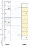 |
Fig. 10 Sub-bucket grouping with interaction distance bounds. The sub-buckets of two buckets A and B and the entities populating them are shown. Sub-bucket indices as per Eq. (110) are indicated in italic type. The arrows indicate: the range of possible A–B interactions, as per the bucket interaction distance bound |

5.4 Bounding the number of possible interactions
Let now nJ,s denote the number of entities in sub-bucket s of bucket J. To compute the upper bound of possibly interacting entity pairs  , we have to iterate through all sub-buckets s in bucket J, obtain the sub-buckets UK,J(s) from bucket K which are in reach of s, and then accumulate the product nJ,snJ,t for all t ∊ UK,J(s):
 (118)
(118)
where we abbreviate the number of entities in bucket K reachable from sub-bucket s of bucket J as
 (119)
(119)
 is commutative,
  , because the notion of being in reach is commutative as stated by Eq. (117). The interval bounds of the sequence of intervals (UK,J(s))s are monotonic, which is to say: a sub-bucket (s + 1) does not reach further back than sub-bucket s, and sub-bucket s does not reach further forward than sub-bucket (s + 1). Therefore, the nested sum can be efficiently computed with a ‘moving window’ scheme. To this end, we iterate over the sub-buckets s of bucket J. For every sub-bucket s, we compute the range of reachable sub-buckets UK,J (s) in bucket K. This range is compared to the range reachable by the previous sub-bucket (s − 1). We compute nK,J,s by taking the previous value nK,J(s−1) and adding and subtracting sub-bucket entity counts nJ,t for sub-buckets t as they fall in and out of reach. As we iterate through the sub-buckets s, we cumulate the product nJ,snK,J,s. If the number of occupied sub-buckets in a bucket J are denoted vJ, computing
  as per Eq. (118) requires only vJ evaluations of the function UK,J(s) and two concomitant passes through the vĸ sub-buckets of bucket K.
When an entity j is updated in Step 3 of the bucketing algorithm, it may have to be moved from one bucket J to another bucket J’ ≠ J, or it may move from sub-bucket s to a different sub-bucket s’ ≠ s of the same bucket J′ = J. In either case, the cumulative values  must be updated, which can be done incrementally. Let
  denote the number of entities to be added (or removed, if δ is negative) to (or from) some sub-bucket
  of some bucket J:
 (120)
(120)
To see how  changes, we subtract the old value
  from the new value
  :
:
 (121)
(121)
If J = K, the  may appear in both of the factors in Eq. (118). We therefore have to distinguish between J = K and J ≠ K. With some algebraic transformations we obtain
 (122)
(122)
where we used the number of reachable entities nK,J,s defined in Eq. (119). Just as the updated quantity  itself, the incremental update
  is commutative,
  . Computing
  is less expensive than recomputing
  , with the cost being near-proportional to the reach of sub-bucket
  .
.
5.5 Sampling
If the global interaction rate bound λ+ (Eq. (102)) is estimated as the sum of products  for buckets J and K, every possible combination of entities j ∊ ℐJ and k ∊ ℐK is considered with the same relative probability. The entity indices j and k can therefore be sampled independently, as done in Step 2.iv of the bucketing algorithm. However, if the sub-bucketing scheme is used, the local upper bound
  (Eq. (101)) is computed instead as the sum of products
  . We must therefore first sample the sub-bucket pairing s, t which contain the interacting entities j, k.
To sample s and t, we first draw a uniformly random integer  . We then use the ‘moving window’ scheme described in Sect. 5.4 to cumulate the sum over nJ,snK,J,s, stopping just before the cumulative value, which shall be denoted ψ, begins to exceed ζ. This determines the sub-bucket s of bucket J from which entity j is taken. Sub-bucket t of bucket K is determined by cumulating values nK,t for all sub-buckets in reach of sub-buckets s until the cumulative value exceeds (ζ − ψ). Once s and t have been determined, entity indices j and k are selected randomly with uniform probability from the arrays of entities held by the sub-buckets s and t.
6 Performance
The efficiency of the bucketing scheme has been studied formally in Sect. 3.7. In this section we empirically assess the computational efficiency of the scheme for two synthetic test cases as well as for a sophisticated physical model which comprises growth by coagulation, viscous stirring, and dynamical friction.
6.1 Linear kernel
In our first test, we simulate a coagulation process with the linear kernel (Eq. (64)) for different numbers of representative particles n using both the traditional inverse transform sampling scheme and the proposed bucketing scheme. Benchmark results for the linear kernel test are reproduced in Fig. 11, which shows the runtime for a single-threaded simulation of the linear kernel until t = 16; the specifications of the benchmark computer are given in Appendix C. For the test we used simple mass bucketing as per Eq. (42) with two buckets per mass decade, θm = 2. The bucketing is very efficient in this case; the average probability of event acceptance is measured to be p ~ 0.18, and the average number of active buckets is 〈v〉 ~ 18, and is only weakly dependent on the value of n.
The gradual decreases in efficiency of the traditional scheme compared to the fitted n2 curve can be correlated with increased memory latency as the size of the simulation data begins to exceed the on-chip caches. This is reasonable, as the computation of interaction rates for the linear kernel is arithmetically trivial (a single addition), which allows us to simplify the cost models of Sects. 2.8 and 3.7 using Cλ ≈ Cop. We thus expect the traditional scheme to run into a bandwidth limit. Conversely, the simulation data required for the bucketing scheme fits the per-socket inclusive L3 cache of our benchmark machine for all values of n examined. Results for the runs with n = 1024 and n = 65 536 are reproduced in Fig. 6, showing increasingly accurate simulation of the desired outcome.
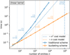 |
Fig. 11 Performance analysis of the linear kernel test for the traditional scheme and the bucketing scheme. The evolution of the linear kernel is simulated until t = 16. The dashed lines show fitted curves for simplified cost models linear and quadratic in n. The vertical dotted lines indicate the number of representative particles n for which the simulation data of either scheme exceeds the sizes of the L1 cache, the per-core L2 cache, the per-socket inclusive L3 cache, and the main memory of the benchmark machine. |
6.2 Runaway kernel
Our second test investigates the runaway kernel (Eq. (70)). Unlike the linear kernel, which we studied in the many-particles regime because the analytical solution assumes continuous particle number densities, the runaway kernel is designed to test the runaway growth of an individual particle, and hence encompasses the transition from the many-particles regime to the few-particles regime. In the extended RPMC method, this transition occurs for a swarm k when the swarm particle count Nk falls below the particle regime threshold Nth. The swarm is then split into Nth individual representative particles each having a swarm particle count of 1 , that is, representing only themselves, and the total number of representative particles n increases accordingly.
The runaway kernel test has scaling characteristics similar to the linear kernel test, as can be seen in Fig. 12, which shows the runtime for a single-threaded simulation of the runaway kernel until t = 70. Because the number of representative particles varies, runtimes are shown for the event-averaged number of representative particles 〈n〉, with the initial and maximal number of representative particles indicated separately. As for the linear kernel, super-quadratic inefficiencies of the traditional scheme can be correlated with the large working set size exceeding the on-chip caches; the interaction rate is almost as trivial to compute as for the linear kernel (assuming that the powers (mk)2/3, which are computationally expensive, have been precomputed and cached for each particle k), so we again expect to eventually be bandwidth-limited. The slightly super-linear runtime of the bucketing scheme for 〈n〉 ≳ 3 × 10⁵ can be attributed to the event-averaged number of occupied buckets 〈v〉 which grows slightly (from ~ 10 to ~ 20) as 〈n〉 increases. The number of occupied buckets increases because, with more representative particles available, more of the tail end of the distribution can be resolved, as is evident from Fig. 7.
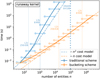 |
Fig. 12 Performance analysis of the runaway kernel test for the traditional scheme and the bucketing scheme. The evolution of the runaway kernel is simulated until t = 70. The dashed lines show fitted curves for simplified cost models linear and quadratic in n. The solid lines show the runtime for the event-averaged number of representative particles. For each tested configuration (solid horizontal lines), the initial number of representative particles (circle) and the maximum number of representative particles in the simulation (right arrow) are indicated. The vertical dotted lines indicate the number of representative particles n for which the simulation data of either scheme exceeds the sizes of the per-core L2 cache, the per-socket inclusive L3 cache, and the main memory of the benchmark machine. |
6.3 Collision and velocity evolution
Although the bucketing scheme was demonstrated to perform substantially better than the traditional implementation for the linear and runaway kernel tests, we note that in these synthetic test cases, entities have only two properties: particle mass and swarm mass. As argued in Sect. 1, one of the main reasons to choose a Monte Carlo method over a grid-based method is that more properties can be added easily, whereas doing so in a grid-based method would increase the dimensionality of the grid, leading to soon-prohibitive costs in terms of both memory and computation resources. The computational scheme traditionally employed for the RPMC method is not sensitive to the dimensionality of the parameter space. This is not necessarily true for the bucketing scheme. If the particle–particle interaction rate is influenced by multiple properties – say, mass and rms velocity –, then the bucketing criterion should consider each of these properties in separate dimensions, similar to what had been done in the refined three-dimensional bucketing criterion in Eq. (43). The bucketing scheme can be likened to a grid method in the subspace of the property space considered by the bucketing criterion; adding an additional property dimension to the bucketing criterion thus adds to the dimensionality of the grid. The curse of dimensionality is somewhat attenuated because the bucketing scheme uses a sparse grid of buckets, but even if the occurrence of different particle properties is perfectly correlated (e.g. a light particle always has a high rms velocity, and a heavy particle is always rather slow) the number of occupied buckets likely increases by some factor for every additional property considered, which can become significant if many additional properties are introduced. To assess the performance of the bucketing scheme with more than one particle property, we therefore turn to a more realistic example.
6.3.1 Ormel’s model
Ormel et al. (2010) have presented a comprehensive stochastic model for the simulation of runaway growth of protoplanetary bodies. The model comprises collisional encounters (leading to coagulation or fragmentation), gravitational interactions (modelled as ‘viscous stirring’ and ‘dynamical friction’, which are stochastic surrogate models for the exchange of kinetic energy between particles), and also gas drag forces and turbulent stirring. Collisional encounters were simulated with the Monte Carlo method of Ormel & Spaans (2008). Gravitational encounters, however, could not be simulated with a Monte Carlo method because of the excessive cost of computing interaction rate updates: ‘[…] it is too demanding to treat collisionless encounters also on an event-based approach. Due to their increased gravitational focusing […] collisionless encounters are more frequent than collisional interactions by several orders of magnitude, especially when the system relaxes to a quasi-steady state in velocity space’ (Ormel et al. 2010, Sect. 2.6).
To test the bucketing scheme in a more likely scenario, we use it to simulate the stochastic growth model introduced by Ormel et al. (2010), henceforth referred to as ‘Ormel’s model’. However, unlike the original implementation, we model both collisional and gravitational encounters as events, which has become feasible thanks to the increased computational efficiency of the bucketing scheme. We simplify the model by neglecting the influence of the gas (effectively setting the gas density to ρgas = 0). Without a gas, there is no turbulent stirring and no gas drag. Apart from this, our model is identical to the model presented in Ormel et al. (2010) save for minute technical details. An extension of Ormel’s model implemented with the bucketing scheme will be elaborated in a forthcoming paper (Beutel et al., in prep.); in the following we shall only briefly summarise the gist of the model before proposing a suitable bucketing criterion.
In our implementation of Ormel’s model, an entity k is equipped with the following properties: swarm mass Mk, particle mass mk, orbital radius rk, planar rms velocity vk, vertical rms velocity υz,k, and solid density ρk. For a representative particle j and a swarm k, the interaction rates for collisions, dynamical friction events, and viscous stirring events are denoted  and
and  . A swarm of particles k is confined to a radial annu-lus of [rk − hx,k, rk + hx,k], where the scale length is given by hx,k = max{Rmin, vk/Ω(rk)} for many-particles swarms (that is, swarms k with Nk > Nth) or by hx,k = vk/Ω(rk) for few-particles swarms (Nk ≤ Nth). Rmin is a simulation parameter which bounds the radial resolution of the simulation, and
  is the Keplerian rotational frequency of a body on a circular orbit around a central object of mass M* with G the gravitational constant. Because swarms are split up at the many-particles → few-particles transition, few-particles swarms contain only a single self-representing particle. Individual particles are not statistical representatives, and therefore imposing a minimal effective scale length is not necessary.
In Ormel’s model, colliding particles can coagulate or fragment. In the very simple collision model parameterised by the effective coefficient of restitution ϵ, outcomes other than coagulation are possible only in the superescape regime, that is, if the approach velocity of the colliding particles exceeds their mutual escape velocity. It is assumed that, upon collision of particles j and k, a fraction ffrag of the combined mass (mj + mk) ends up as fragments. For simplicity, a uniform fragment size of Rfrag = 1 cm is assumed (slightly different from Ormel et al. (2010) who used Rfrag = 1 mm and Rfrag = 10 cm). The mass fraction depends on the particle masses and the kinetic energy of the impact,
 (123)
(123)
where  is the mutual escape velocity, and where the kinetic energy of the impact is
 (124)
(124)
with va the particle approach velocity.
For the three types of interaction – collisions, viscous stirring, dynamical friction –, the interaction radii  can be computed; two entities j, k can only interact if the particles they represent can get closer than the respective interaction radius. Interaction rate, interaction radius, and interaction outcome are also dependent on the velocity regime. Interactions of particles with low rms velocities operate in the shear-dominated regime, whereas a higher rms velocity places the interaction in the dispersion-dominated regime. A pair of particles with a stochastic relative velocity faster than their mutual escape velocity is in the superescape regime where viscous stirring and dynamical friction are irrelevant and where the effect of gravitational focussing is negligible.
Determining interaction rates or interaction radii for either type of interaction is complicated. Among other things, for a representative particle j and a swarm k the geometric overlap of the ‘living zones’ of the two swarms has to be computed, and the routines contain multiple if-else branches to distinguish between the different velocity regimes. In contrast to the synthetic linear and runaway kernel test cases of Sects. 6.1 and 6.2, the computation of interaction rates thus costs much more than a single arithmetic operation, Cλ ≫ Cop, which means that the simulation remains compute-bound for much larger working-set sizes than with the synthetic tests.
For the bucketing scheme, an interval extension of the interaction rate function is required. Due to the inherent complexity of the interaction rate function, constructing a corresponding interval extension by hand would be very laborious and error-prone. Instead, we use the interval-aware programming paradigm of Beutel & Strzodka (2023) to implement the routines for computing interaction rates such that they can return either a real value for real-valued input arguments or an interval for interval-valued input arguments.
For all but the simplest operations, interval arithmetic is disproportionately expensive compared to real arithmetic. As an example, computing the sum of two intervals requires only two additions, but computing the product of two intervals requires at least four multiplications, three min, and three max operations (cf. e.g. Hickey et al. 2001). As a result, the estimation of a bucket-bucket interaction rate upper bound is notably costlier than the computation of a particle-swarm interaction rate,  . As per the cost models in Eqs. (26) and (61), it is thus possible that the traditional scheme outperforms the bucketing scheme for relatively small numbers of representative particles, n ~ v.
To test the bucketing scheme with Ormel’s model, we adopt the following test scenario, which is a gas-free version of the 1 AU test case in Ormel et al. (2010). We simulate a protoplan-etary system with a central star of solar mass, M* = M⊙ with a narrow annulus at a0 = 1 AU of width ∆a = 0.04 AU that is uniformly populated by protoplanetary objects of initial mass m0 = 4.8 × l018 g and solid density ρ = 3 g/cm3. The mass surface density inside the ring is ∑0 = 16.7 g/cm2. The particles have an initial rms velocity of υ0 = 4.7 × 102 cm/s. The gas density is assumed to be ρgas = 0 for simplicity. To avoid under-sampling, the radial resolution of the simulation is constrained by Rmin = ∆a/64. The simulation is then run for a duration of 1.8 × 10⁵ years of simulated time, modelling the interplay of particle coagulation and velocity evolution as a series of individual events. We test the model with two different values for the coefficient of restitution: ϵ = 0, which implies that no fragmentation occurs and collisions always lead to coagulation; and ϵ = 0.01, a value corresponding to a ‘rubble pile’ model of planetesimals (Ormel et al. 2010, Sect. 2.5.2).
The test particles are sampled with n randomly chosen representative particles, where n is varied during different simulation runs. Every representative particle k initially represents an equal-weight fraction of the total mass, Mk = ℳ/n, where the total mass is
 (125)
(125)
In the bucketing criterion, all properties which quantitatively affect the interaction rate are considered separately:
 (126)
(126)
where C(q) is the swarm regime classifier defined in Eq. (44), particle mass, swarm mass, and planar and vertical rms velocities of a representative particle with properties q are given by m(q), M(q), v(q), and vz(q), respectively, and where the simulation parameters θm, θM, and θv control the number of buckets per decade of the respective quantity. Unless indicated otherwise, we adopt the values θm = θM = 6, θv = 5. Ormel’s model is employed to study runaway growth, which means that some representative particles transition into the few-particles regime where individual particles can absorb up the mass of other swarms. Following the discussion in Beutel & Dullemond (2023), we adopt a particle regime threshold of Nth = 10.
The described physical system is not homogeneous. From the range-limited stirring and coagulation processes, structures emerge on certain length scales, and therefore spatial resolution is required so these structures can be properly resolved. We therefore take advantage of the sub-bucketing extension of the bucketing scheme introduced in Sect. 5. In our simulations, we use a sub-bucket granularity of dmin = 8. Because the interaction radii tend to scale with the orbital radius, we adopt the logarithmic definition of the interaction distance given in Appendix B.
6.3.2 Boosting
As assessed by Ormel et al. (2010), the number of events that need to be simulated is vast because ‘[…] the MC code does not recognize that the collective effect of these encounters cancels out, but instead resolves the strongly fluctuating velocities of the bodies, which render the code very inefficient’ (Ormel et al. 2010, Sect. 2.6, cont’d). Although the MC simulation of the velocity evolution becomes feasible with the bucketing scheme, the general inefficiency of the model remains. However, the model can be made more efficient by applying the boosting technique, previously described for coagulation in the companion paper (Beutel & Dullemond 2023), to stirring and friction events. With boosting, gravitational interactions which transport minuscule amounts of kinetic energy are grouped together, decreasing the rate while correspondingly increasing the kinetic energy transfer. Although this is an approximation, it does not impair the main benefit of simulating gravitational interactions with a Monte Carlo method, which is that sudden discrete changes of kinetic energy (a heavy particle ‘kicking’ a light one) can be modelled correctly. Unless noted otherwise, we apply the boosting technique to all our simulations of Ormel’s model for collision events as well as for viscous stirring and dynamical friction, using a mass growth rate of 5% and an rms velocity change rate of 2%.
6.3.3 Results
A typical result obtained with the simplified Ormel’s model showing the emergence of oligarchs is reproduced in Fig. 13 with three snapshots at t = 1.3 × 10⁴ yr, t = 3.8 × 10⁴ yr, and t = 1.8 × 10⁵ yr. Results for two runs with ϵ = 0 (no fragmentation) and ϵ = 0.01 (corresponding to a rubble pile model) are shown.
When comparing the results to Fig. 9 of Ormel et al. (2010), we note that the distribution structure of the colour-encoded dynamical temperature visibly differs; in particular, the correlation between particle size R and rms eccentricity seems absent in our result. This may be due to the negligence of the gas disk in our simplification of Ormel’s model. A gas disk would orbit the central body at a lower orbital velocity and thus exert a gas drag force which effectively damps the rms eccentricities and rms inclinations of massive bodies (cf. Inaba et al. 2001). The damping rate of a body is correlated with its surface-to-volume ratio, and thus damping is more effective for smaller bodies, an effect that can be observed in Fig. 9 of Ormel et al. (2010) but not in our results. Another difference is the slight radial compaction visible in our results, which stems from the fact that, in our simulation, the boundaries in the radial dimension r are unconstrained, whereas Ormel et al. (2010) used periodic boundaries.
Including fragmentation has the obvious consequence that some mass is removed from the swarms of planetesimal-sized bodies. Fragments are assumed to be tightly coupled to the gas (the presence of which we conceptually assume even though we ignore its other effects here), and hence they neither self-accrete nor contribute to viscous stirring or dynamical friction. Instead, they are available as a mass reservoir for accreting planetesimals. This leads to a visible dissipation of masses in the lower end of the mass distribution. With fragmentation, the emerging oligarchs grow to slightly larger masses in the same amount of time, an observation consistent with Fig. 10 of Ormel et al. (2010).
The dashed vertical lines in Fig. 13 indicate the spherical particle radius
 (127)
(127)
corresponding to the critical mass mcrit defined as
 (128)
(128)
(cf. Beutel & Dullemond 2023, Eq. (39)). This mass segregates many-particles and few-particles swarms under the simplifying assumption that there are n0 swarms which all represent an equal fraction of the total mass, Mk = ℳ/n0 ∀k. Representative particles with a mass greater than mcrit tend to be few-particles swarms, and because the RPMC method splits up swarms once their particle number falls below the particle number threshold Nth, such particles then are self-representing. The corresponding increase of resolution is visible in the vicinity of mcrit.
Although the geometric model employed by Ormel et al. (2010) for collisions, viscous stirring and dynamical friction works well as a statistical model for swarms comprising many particles, its assumptions break down for interactions between individual particles which have individual, not statistical, orbital properties. Specifically, features such as orbital resonances or radial redistribution cannot be reproduced with the geometric interaction model. Therefore, self-representing bodies exceeding a certain mass should be simulated with an N-body code. The inclusion of an N-body code exceeds the scope of this work, so we follow Ormel et al. (2010) in unconditionally applying the statistical interaction models for all swarms k regardless of their particle mass mk or particle count Nk.
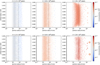 |
Fig. 13 Results for the simplified Ormel’s model starting with n0 = 32 768 representative particles. Top row: ϵ = 0 (no fragmentation); bottom row: ϵ = 0.01 (rubble pile model). Every swarm is represented by a spherical shape with a colour indicating its planar rms eccentricity. The area covered by the shape represents the mass in the swarm. All swarms initially have the same mass, but individual particles can accrete mass held by other swarms and thereby grow beyond their initial swarm size. The vertical lines indicate the critical radius Rcrit (Eq. (127)) which marks the approximate boundary between many-particles and few-particles swarms. |
6.3.4 Performance
Although the runtime performance is no longer dominated by memory access times, the memory usage of the simulation poses a practical constraint for the possible scaling. In Fig. 14, the memory cost of simulating Ormel’s model is explored for a variety of representative particle counts n and occupied bucket counts v. It is evident that the traditional scheme soon exhausts the available memory when increasing resolution beyond n = 103 representative particles. In contrast, the memory cost of the bucketing scheme is much lower overall and scales with n⋅v2. To understand the kinks, we remember that buckets are allocated sparsely; because each entity is assigned to one and only one bucket, the number of entities n acts as an upper bound to the number of occupied buckets v.
A performance analysis of Ormel’s model comparing the traditional scheme and the bucketing scheme is reproduced in Fig. 15. The bucketing scheme again performs substantially better than the traditional scheme. Because of the relatively high bucket density chosen with θm = θM = 6, θv = 5, the number of occupied buckets v is large (saturating around v ~ 350), and thus the cost for bucket updating is relatively high even for a small number of entities n. However, the computational cost grows only weakly as the number of entities n increases, even bettering the scaling behaviour predicted by the cost model of Sect. 3.7, as demonstrated by the ad hoc ~ n2/3 cost model fit which seems to closely match the observed simulation performance.
Our analytical cost model does not explain the apparent sub-linear scaling of the bucketing scheme observed in Fig. 15. It is possible that the scaling may ultimately become linear in n, as predicted by the cost model, for even larger values of n which we did not test. We note, however, that we have not investigated the cost impact of the sub-bucketing extension of our scheme, which might cause the different scaling characteristics. An extended cost model would have to entail some analytical representation of the effects of constrained reachability, which we found difficult enough to eschew the effort.
The spatial resolution of the system is limited by the simulation parameter Rmin, which here was chosen as Rmin = ∆a/64. Because we want to investigate the scaling behaviour of the bucketing scheme, this simulation parameter has remained invariant over all simulation parameter sets. Normally, this parameter would be chosen such as to avoid undersampling, which implies that it would be inversely proportional to the number of representative particles used, Rmin ∝ n−1. Choosing a larger Rmin for smaller n would imply that swarms may be effectively spread out farther, allowing interactions between particles farther apart, and therefore allowing more interaction events and presumably slowing down the simulation. Conversely, choosing a smaller Rmin for larger n, and thereby increasing the resolution of the simulation, would allow swarms to occupy narrower annuli, and thus decrease the number of interaction events because more particle pairings would be out of reach. Reducing Rmin for larger n would thus presumably speed up the simulation. We also note that, even without explicitly reducing Rmin, spatial resolution improves with increasing n because, as explained in Sect. 6.3.1, Rmin is not imposed as a minimum effective scale length for particles which are represented individually; with more representative particles available to sample the system, the transition to individual particles occurs at lower masses, and therefore at an earlier time. This effect may also play into the sub-linear efficiency scaling observed.
The average number of occupied buckets shown in the bottom panels of Fig. 15 steadily increases at first, then seems to saturate for n ≳ 4 × 10³ (and begins to decrease slightly for larger n), indicating, though not conclusively proving, that n ≳ 4 × 10³ representative particles may be sufficient in covering the full dynamic range of the system, and, conversely, that the system may suffer from undersampling for n ≲ 4 × 10³. After the average number of occupied buckets plateaus for 4 × 10³ ≲ n ≲ 105, it again begins to grow for n ≳ 105. This may indicate that the system is ‘over-resolved’: by increasing n0, the critical mass mcrit (Eq. (128)) of regime transition is reduced, and swarms become few-particles swarms already at lower particle masses. By its design, the original RPMC method has a self-balancing property: all swarms retain the fraction of the total mass they were initialised with. Specifically, in an equal-weight sampling, every swarm k would be initialised with the same fraction Mk = ℳ/n of the total mass ℳ, and therefore the ensemble of swarms would always remain an equal-weight sampling, which is beneficial because it maximises the sampling efficiency. In the extended RPMC method, the self-balancing property could be retained only for many-particles swarms. Therefore, by excessively increasing the resolution, and in turn by pushing the critical mass mcrit of regime transition far below the threshold mass for runaway growth, the statistical self-balancing property is gradually lost, leading to an increase in the average number of occupied buckets, which in turn slightly impairs the scaling characteristics.
As is evident from Fig. 15, the inclusion of a fragmentation model does not significantly affect the performance characteristics of the bucketing scheme. It was mentioned in the companion paper (Beutel & Dullemond 2023, Sect. 7) that the RPMC method, the same as any Lagrangian method, is ‘ill-suited for simulating “stiff” problems in which two adverse effects nearly balance each other’. One could imagine a system with a steady-state mass distribution which nevertheless exhibits active growth and fragmentation; in such a system, a Lagrangian method has to follow the individual particles as they cycle through the growth and fragmentation process. This is, however, not the case in our fragmentation test: although mass is exchanged in both directions (planetesimals collide and form fragments, and fragments are accreted by planetesimals), the system does not have steady-state characteristics; instead, the system steadily evolves towards larger bodies (oligarchs) which eventually become dynamically isolated and thus are unlikely to fragment further.
The companion paper also elaborates that the ‘stiffness’ problem is aggravated by the proposed extension of the RPMC method because swarms that repeatedly follow the growth-fragmentation cycle may be repeatedly split up over the course of the simulation, leading to a steady growth in the number of representative particles. The companion paper subsequently proposes that a merging step be incorporated to counteract the problem when simulating a system with steady-state characteristics. This advice remains appropriate with the bucketing scheme, although we note that the nature of the bucketing scheme helps reduce the cost induced by unnecessarily splitting up swarms since swarms with similar characteristics typically end up in the same bucket.
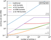 |
Fig. 14 Memory cost analysis of simulating Ormel’s model. The dashed and solid lines show the memory required for simulating Ormel’s model with the traditional implementation and the bucketing scheme, respectively. Some cache sizes and the main memory size of the benchmark machine are indicated with horizontal dotted lines. |
6.3.5 Impact of simulation parameters
The simulation parameters θm, θM, and θv, representing bucket densities in the respective dimensions of the space of bucket labels, need to be chosen large enough that the bucket-bucket interaction rate upper bounds are not excessive, which would lead to a very high probability of rejection and render the sampling process inefficient. At the same time, said parameters must be chosen as small as possible so as to minimise the total number of buckets occupied, and thereby minimise the cost of updating buckets and recomputing bucket–bucket interaction rates.
Figure 16 demonstrates how these contradicting requirements lead to a practical trade-off. In the first panel, we see that, by increasing bucket densities, resulting in narrower bucket parameter intervals, we can improve the quality of the bucket–bucket interaction rate bounds. With better bounds, the likelihood of rejection is lower, and the average probability of event acceptance p is higher. If fewer events need to be sampled only to be ultimately rejected, the simulation should run faster. In the second panel we can see, however, that the increased number of buckets which results from choosing a higher bucket density increases the cost of bucket updates, which at some point exceeds the gains from a higher acceptance probability. For the given set of parameters, a good choice for bucket density might thus be θv = θm = θM = 5.
If similar events of low impact are aggregated, as done by the boosting technique mentioned in Sect. 6.3.2, the benefit of bucket widening is negligible. The simulation results in Figs. 15 and 16 have been run with boosting enabled. In these simulations, widening has proved unnecessary, and hence a widening fraction of f = 0 has been adopted. However, if the simulation is run without boosting, viscous stirring and dynamical friction events abound, rendering the simulation substantially slower. Widening can be useful in this situation, as demonstrated by Fig. 17. The bucketing scheme is very efficient in this case, yielding average acceptance probabilities of p ~ 40%; however, because of the exorbitant number of events, a single simulation run takes between one and two hours to complete even though the width of the annulus has been reduced and the number of representative particles is relatively low. (A simulation employing the traditional scheme did not complete within the 8 h time limit of our benchmark machine.) Simulating viscous stirring and dynamical friction events as Monte Carlo events without boosting, albeit possible with the bucketing scheme, is thus not very practical.
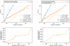 |
Fig. 15 Performance analysis of Ormel’s model for the traditional scheme and the bucketing scheme with boosted dynamical friction and viscous stirring. Left column: ϵ = 0 (no fragmentation); right column: ϵ = 0.01 (rubble pile model). In the top panels, the dashed lines show fitted curves for simplified cost models linear and quadratic in n, and an additional ad hoc fit with a n2/3 proportionality. The solid lines show the runtime for the event-averaged number of representative particles. For each tested configuration (solid horizontal lines), the initial number of representative particles (circle) and the maximum number of representative particles in the simulation (right arrow) are indicated. The bottom panels show the average number of occupied buckets for each of the simulation parameter sets. |
7 Discussion
For the synthetic test cases of Sects. 6.1 and 6.2, the proposed scheme shows a clear performance advantage over the traditional scheme. However, in the case of a more realistic test case simulating the interplay of multiple effects such as hit-and-stick coagulation and gravitational stirring, as studied with Ormel’s model in Sect. 6.3, we note that the high dimensionality of the parameter space poses a challenge for the bucketing scheme. For competitive performance, we had to adapt the bucketing criterion of Eq. (126) which gave rise to a five-dimensional space of bucket labels and use relatively high bucket densities θm, θM, θv, resulting in a relatively large number of ~450 occupied buckets on average. Even with a high-dimensional bucketing criterion and a high bucket density, the bucketing scheme has substantially outperformed the traditional scheme for larger entity counts n, showing superior and even sub-linear scaling characteristics for the range of parameters tested.
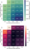 |
Fig. 16 Parameter study of the bucket densities θv, θm, θM in Ormel’s model. The two panels show the average probability of event acceptance p and the per-event runtime cost, respectively, as functions of the rms velocity bucket density θv and the mass bucket densities θm = θM. The simulation uses the setup described in Sect. 6.3.1 with boosting, as in Fig. 15, for an initial number of n0 = 4096 representative particles. |
7.1 Limitations
Although we advertise the bucketing scheme as a general-purpose computational scheme for Monte Carlo simulations of compound Poisson processes, there are some practical limitations to its usefulness. The most obvious limitation is the conceptual complexity of the scheme, which makes it challenging to implement. We hope to alleviate this concern somewhat by subsequently publishing our implementation, written in C++20 and designed with reusability in mind, as an open-source software package. Nevertheless, a user of the package needs to understand how the scheme works in order to use it effectively.
Another requirement that may be challenging to satisfy is the need for an interaction rate function which can either operate on real values or on intervals. Although software packages for interval arithmetic are available (e.g. Brönnimann et al. 2006; Goualard 2015) and recent work has been advancing a notion of interval-aware programming (Beutel & Strzodka 2023), devising an efficient interval extension of an arbitrary calculation is an unsolved problem and requires thorough mathematical study of the calculation and meticulous avoidance or containment of the so-called dependency problem that is inherent to interval arithmetic (e.g. Gustafson 2017, Sect. 16.2f).
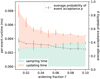 |
Fig. 17 Parameter study of the widening fraction ƒ in Ormel’s model without boosting. For this test, the width of the annulus was reduced to ∆a = 0.0025 AU, fragmentation was suppressed (e = 0), and the system was sampled with an initial number of n0 = 128 representative particles. |
7.2 Possible improvements
The lower memory requirements of the bucketing scheme allow to push the boundaries of our simulation much further than would be possible with the traditional scheme, as outlined in Fig. 14. In addition, the bucketing scheme outperforms the traditional scheme in every scenario tested, often scaling with n as opposed to the n2 scaling of the traditional scheme. Nevertheless, our tests also expose some limitations of the bucketing scheme. An obvious limitation is the sequential nature of the algorithm. Also, as we saw in Sect. 6.3.5, selecting an efficient set of simulation parameters is not easy and may require a parameter study.
It had been argued in Sect. 3.7 that the cost rate of the bucketing scheme scales at least quadratically in the number of occupied buckets v; therefore, if the bucket density is chosen such that v is large, the cost of the simulation can be very high even for moderate entity counts n, and higher than the cost of the traditional scheme due to the greater cost and the excess of interval-valued calculations. This can be observed at the lower end of Fig. 15: in a run with an initial number of n0 = 512 representative particles, the bucketing scheme even performs slightly worse than the traditional scheme. We note that this run is not meaningful physically because the system is severely undersampled with only n0 = 512 representative particles; still, we would want to better the traditional scheme with a significant margin even for smaller entity counts n. We saw in Sect. 6.3.5 that the bucket density must be chosen as a trade-off between a lower number of occupied buckets v and low rejection rates due to tighter estimates for the bucket-bucket interaction rate. This trade-off plays out differently for different entity counts n, and indeed the simulation with n0 = 512 could have been sped up by selecting lower bucket densities. Our observations raise the question of whether and how the scheme could be improved towards better performance without having to conduct parameter studies and tuning of simulation parameters.
7.2.1 Parallelisation
Our reference implementation of both the traditional scheme and the bucketing scheme is a sequential code. It runs in a single thread and does not take advantage of modern multi-core processors or massively parallel architectures such as GPUs. Although the proposed design of the scheme is of inherently sequential nature due to the global ordering of events, the two main simulation steps – sampling an event and recomputing bucket–bucket interaction rate upper bounds – could be parallelised straightforwardly. In the vernacular of parallel computing, the updating step would be considered ‘embarrassingly parallel’. In the sampling step, the overhead caused by rejection sampling could be mitigated by sampling P events concurrently, where P ∈ ℕ+ is the degree of parallelism desired, and discarding all but the first of the sampled events that were not rejected.
In parallel computers, synchronising state globally is a very expensive operation. When pushing the simulation to larger scales, the global ordering of the events will eventually become a bottleneck. A massively parallel computational scheme would presumably want to employ a ‘divide and conquer’ approach, assigning a fraction of the total particle ensemble to each worker. The forgiving nature of the bucketing scheme – its tolerance of minute changes of entity properties within the bucket property bounds – would prove beneficial in the inevitable merging of concurrently simulated events.
7.2.2 Adaptive bucketing
In all bucketing criteria proposed so far, the number of buckets per decade (or the linear equivalent) had to be chosen explicitly as a simulation parameter. Choosing appropriate simulation parameters requires some knowledge of the simulated model, and often some parameter study as well. But with a set of simulation parameters that assures reasonably efficient rejection sampling, the total number of buckets required can be too large, rendering bucket updates very costly.
However, the number of buckets per decade need not be fixed. Different parameter values could be used over the course of the simulation, or even for different decades. In fact, the way the bucketing scheme is constructed, the bucketing criterion B(q) can return an arbitrary result without impairing the correctness of the simulation; in particular it may return different results when called at different times. Specifically, B(q) could also refer to some global state g (such as the current simulated time) or to simulation state s (such as the current number of occupied buckets) and should thus be written B(q, g, s). Using this freedom, a bucketing criterion could incorporate a feedback loop. For example, for every bucket J currently occupied we could maintain a running average of the number of rejections required to sample an event for a representative particle in this bucket. If the required number of rejections, weighted by the relative interaction rate weight of the bucket
 (129)
(129)
is low (a good reference value might be 2nJ, the number of updates that would need to be computed had the traditional scheme been used inside the bucket instead of rejection sampling), the bucketing criterion may ‘zoom out’, locally coarsening the bucketing criterion and thereby allowing the bucket to be merged with adjacent buckets which also have been zoomed out of. Conversely, if the required number of rejections is very high in a zoomed-out bucket, then the bucketing criterion would ‘zoom in’, thus redistributing all entities in the bucket to finer-grained buckets. Simulation parameters such as θm, θM, θv would be retained, but they would only set the highest possible resolution of the bucketing criterion.
8 Summary and conclusions
We have presented a novel computational scheme for the simulation of a stochastic process. The scheme combines a variant of the traditional sampling scheme with rejection sampling by grouping entities in a sparse grid of buckets, applying the discrete inverse transform sampling scheme to the buckets, and then selecting entities by means of rejection sampling. The scheme is made generally applicable by employing interval arithmetic to compute interval-valued interaction rates. It was shown to outperform the traditional scheme in terms of computational complexity and memory requirement as well as in practical performance and scalability for a variety of numerical tests.
In Sect. 2, we recounted how a stochastic process may be simulated with the traditional scheme that can be traced back to Gillespie (1975). A cost model for memory and computational resources was derived in Sect. 2.8. The bucketing scheme was then introduced in Sect. 3. The simulation algorithm and the associated data structures were defined in Sects. 3.5 and 3.6, and a cost model for the bucketing scheme was derived in Sect. 3.7. Section 4 discussed the matter of computing interaction rate bounds with interval arithmetic, along with strategies to increase the efficiency of the updating step. In order to exploit the locally constrained nature of most physical interaction models, we then introduced the notion of sub-bucketing in Sect. 5. In Sect. 6, we test the bucketing scheme for two simple synthetic test cases and one more realistic elaborate model based on Ormel et al. (2010), finding superior performance and scaling characteristics with regard to the number of representative particles n in all cases. Some parameter studies regarding the simulation parameters were then conducted in Sect. 6.3.5.
Our companion paper (Beutel & Dullemond 2023) had extended the RPMC method to allow for smooth transition into the runaway growth regime where bodies need to be treated individually. The transition happens abruptly: a swarm of Nth particles is replaced with Nth individual self-representing particles. Mitigating the performance impact of adding new representative particles to a RPMC simulation, which the original RPMC method of Zsom & Dullemond (2008) had been designed to avoid, was the original goal of devising the bucketing scheme. With the proposed scheme, representative particles can now be added and removed at amortised constant computational cost. According to our cost model, the simulation cost rate scales with n ⋅ v with the number of buckets v at most weakly dependent on n, which is substantially better than the traditional scheme for which the cost rate is proportional to n2. The predicted scaling behaviour has been found to be accurate in simple homogeneous test cases. In our study of a complex test case with spatial resolution, we found the cost rate of the bucketing scheme to scale even sub-linearly with n.
Acknowledgements
We would like to thank Til Birnstiel, Sebastian Stammler, Joanna Drażkowska, and Christoph Klein for valuable feedback and useful discussions. We also thank the anonymous referee, whose substantiated comments and enquiries led us to a flaw in our test case, and overall helped us greatly improve the clarity of the paper. This work is funded by the Deutsche Forschungsgemeinschaft (DFG, German Research Foundation) under Germany’s Excellence Strategy EXC 2181/1-390900948 (the Heidelberg STRUCTURES Excellence Cluster).
Appendix A Interval arithmetic
It is commonplace in mathematical notation to apply scalar functions to sets, as in
![Mathematical equation: $\sin = [ - 1,1].$](/articles/aa/full_html/2024/04/aa47304-23/aa47304-23-eq218.png) (A.1)
(A.1)
Such notation makes implicit use of the intuitive set extension, which could be defined for some scalar function f : 𝒟 → ℝ and for some subdomain 𝒮 ⊆ 𝒟 as
 (A.2)
(A.2)
Although convenient in formal reasoning, computation with general sets is not feasible numerically because there is no obvious closed-form representation for arbitrary sets. However, we can construct a similar technique that is practically computable by constraining ourselves to closed intervals, that is, closed connected subsets of R. Intervals can be represented numerically as an ordered tuple of two numbers a and b with a ≤ b, which constitute the lower and upper bound of the interval. The corresponding closed interval is usually referred to as [a, b].
Let us first introduce some notation. We denote the set of all intervals in some closed connected subset  of the affinely extended real numbers
  as
as
![Mathematical equation: $[{\cal S}]: = \{ [a,b]:a,b \in {\cal S},a \le b\} .$](/articles/aa/full_html/2024/04/aa47304-23/aa47304-23-eq222.png) (A.3)
(A.3)
We shall henceforth denote interval-valued quantities as [x], identifying the bounds of a closed interval [x] as
![Mathematical equation: $[x] \equiv \left[ {{x^ - },{x^ + }} \right],$](/articles/aa/full_html/2024/04/aa47304-23/aa47304-23-eq223.png) (A.4)
(A.4)
and also use an analogous shorthand notation for vector-valued quantities v ∈ ℝu,
![Mathematical equation: $[{\bf{v}}] \equiv \left[ {{{\bf{v}}^ - },{{\bf{v}}^ + }} \right],$](/articles/aa/full_html/2024/04/aa47304-23/aa47304-23-eq224.png) (A.5)
(A.5)
where an interval of vector-valued quantities [v−, v+] is understood as the Cartesian product of element-wise intervals,
![Mathematical equation: $\left[ {{{\bf{v}}^ - },{{\bf{v}}^ + }} \right]: = \left[ {v_1^ - ,v_1^ + } \right] \times \cdots \times \left[ {v_u^ - ,v_u^ + } \right],$](/articles/aa/full_html/2024/04/aa47304-23/aa47304-23-eq225.png) (A.6)
(A.6)
and where the u-dimensional space of vectors of intervals is denoted as ![Mathematical equation: ${\left[ {\overline } \right]^u}$](/articles/aa/full_html/2024/04/aa47304-23/aa47304-23-eq226.png) .
.
For some real-valued function  defined on a subset
  , any function
 ![Mathematical equation: $F:[{\cal S}] \to [\overline ]$](/articles/aa/full_html/2024/04/aa47304-23/aa47304-23-eq229.png) shall be called an ‘interval extension’ of f if
shall be called an ‘interval extension’ of f if
![Mathematical equation: $f(x) \in F([x])\forall x \in [x]\forall [x] \in [{\cal S}],$](/articles/aa/full_html/2024/04/aa47304-23/aa47304-23-eq230.png) (A.7)
(A.7)
that is, F is an interval extension of a function f if, for every interval [x], the interval F([x]) contains the value f(x) for every value x in the interval [x].
Closed-form interval extensions can be defined for all elementary arithmetic operations. For example, for addition and negation:
![Mathematical equation: $[x] + [y]: = \left[ {{x^ - } + {y^ - },{x^ + } + {y^ + }} \right],$](/articles/aa/full_html/2024/04/aa47304-23/aa47304-23-eq231.png) (A.8)
(A.8)
![Mathematical equation: $ - [x]: = \left[ { - {x^ + }, - {x^ - }} \right].$](/articles/aa/full_html/2024/04/aa47304-23/aa47304-23-eq232.png) (A.9)
(A.9)
For any monotonically increasing function  , an exact interval extension is given by
![Mathematical equation: $G([x]) = \left[ {g\left( {{x^ - }} \right),g\left( {{x^ + }} \right)} \right].$](/articles/aa/full_html/2024/04/aa47304-23/aa47304-23-eq234.png) (A.10)
(A.10)
A theorem often referred to as the ‘Fundamental Theorem of Interval Arithmetic’ states that, given a closed-form real-valued arithmetic expression composed of real-valued arguments, an interval extension can be obtained by syntactically replacing every real-valued function and operator with its interval extension (e.g. Hickey et al. 2001). In practice, this means that interval extensions are composable: if some real-valued function f has an algebraic closed-form definition for whose building blocks (such as elementary arithmetic operations) interval extensions are known, then an interval extension of f can be constructed with a syntactic transformation.
Appendix B Logarithmic location and distance
Let an interaction radius function R(q, q′) be given as defined in Sect. 5. Further, let the position of entity j be given by aj ≡ a(qj). Let us also assume that interaction radii approximately scale with the position. As an example, forrepresentative particles j, k in a protoplanetary disk where the rms velocities are low (the Hill regime), the interaction radius for collisions might be determined by the dimensionless Hill radius  ,
,
 (B.1)
(B.1)
where  is the geometric average of the semimajor axes of representative particles j and k. With a non-local bucketing scheme such as Eq. (126), two representative particles j, j′ of equal mass mj = mj′ but located at different semimajor axes
  ·end up in the same bucket J. For a lighter particle k, mk < mj, the interaction radii would therefore differ, Rcoll,j′k > Rcoll,jk. For a bucket K of lighter particles,
  , the bucket-bucket interaction radius bound
  would then be excessive for particle j, and may thus lead to tentative collision events between particles too far apart which will ultimately be rejected.
To avoid this, we define locations and interaction distances as scale-free quantities. First, we define the scale-free interaction width
 (B.2)
(B.2)
A scale-free definition of location can be given as
 (B.3)
(B.3)
with a normalisation factor γ to be defined later.
To define the distance measure d(q, q′), we first recall that two particles with properties q and q′ can interact only if their impact parameter, estimated as b ≥ |a − a′| as per Eq. (95), is not greater than their interaction radius,
 (B.4)
(B.4)
The interaction range of some particle with properties q thus is the interval of semimajor axes [a′] of particles with properties q′ with which interaction may be possible.
Now let us assume that, rather than the interaction radius R(q, q′), the interaction width ω(q, q′) is known, where
 (B.5)
(B.5)
Inserting Eq. (B.5) into Eq. (B.4), we thus find the interaction range for some particle at semimajor axis a and interaction width ω to be defined implicitly by
 (B.6)
(B.6)
Solving Eq. (B.6) for a′ yields
![Mathematical equation: ${a^\prime } \in a\left[ {1 + {1 \over 2}{\omega ^2} \pm \omega \sqrt {{{{\omega ^2}} \over 4} + 1} } \right].$](/articles/aa/full_html/2024/04/aa47304-23/aa47304-23-eq246.png) (B.7)
(B.7)
where we again use sloppy interval notation, [x ± y] = [x − |y|, x + |y|].
The interaction distance d(q, q′) is defined by the Euclidean relation of Eq. (106). We insert Eq. (B.3) and take the values of a′ farthest from α at which interaction could possibly occur as per Eq. (B.7), finding
 (B.8)
(B.8)
where we abbreviated ω ≡ ω(q, q′). The normalisation factor γ is then defined by relating the minimum interaction width
 (B.9)
(B.9)
which represents the smallest length resolved by the simulation at the reference radius, to an interaction distance of dmin:
 (B.10)
Appendix C Benchmark computer specifications
The performance benchmarks shown in Figs. 11, 12 and 15 were run as exclusive single-threaded jobs on machines with one CPU of type Intel Xeon E3-1585 v5 (Skylake-H, 4 cores, 3.5–3.9 GHz) and with 64 GiB of random-access memory.
The parameter studies shown in Figs. 16 and 17 were run as concurrent single-threaded jobs on machines with one CPU of type AMD Epyc 7662 (Zen 2, 64 cores, 2-3.3 GHz) and with 256 GiB of random-access memory.
Appendix D List of symbols
A cross-referenced overview of the most commonly used symbols in this work is given in Table D.1.
List of commonly used symbols.
References
- Alefeld, G., & Herzberger, J. 2012, Introduction to Interval Computation (Academic Press) [Google Scholar]
- Armitage, P. J. 2007, arXiv e-prints [arXiv:astro-ph/8781485] [Google Scholar]
- Beutel, M., & Dullemond, C. P. 2023, A&A, 670, A134 [NASA ADS] [CrossRef] [EDP Sciences] [Google Scholar]
- Beutel, M., & Strzodka, R. 2023, in Next Generation Arithmetic, eds. J. Gustafson, S. H. Leong, & M. Michalewicz, Lecture Notes in Computer Science (Cham: Springer Nature Switzerland), 38 [CrossRef] [Google Scholar]
- Brauer, F., Dullemond, C. P., & Henning, T. 2008, A&A, 480, 859 [NASA ADS] [CrossRef] [EDP Sciences] [Google Scholar]
- Brdar, S., & Seifert, A. 2018, J. Adv. Model. Earth Syst., 10, 187 [NASA ADS] [CrossRef] [Google Scholar]
- Brönnimann, H., Melquiond, G., & Pion, S. 2006, Theoret. Comput. Sci., 351, 111 [CrossRef] [Google Scholar]
- Dullemond, C. P., & Dominik, C. 2005, A&A, 434, 971 [CrossRef] [EDP Sciences] [Google Scholar]
- Dziekan, P., & Pawlowska, H. 2017, Atmos. Chem. Phys., 17, 13509 [CrossRef] [Google Scholar]
- Gillespie, D. T. 1975, J. Atmos. Sci., 32, 1977 [NASA ADS] [CrossRef] [Google Scholar]
- Goualard, F. 2015, GAOL (Not Just Another Interval Library) [Google Scholar]
- Grabowski, W. W., Morrison, H., Shima, S.-I., et al. 2019, Bull. Am. Meteorol. Soc., 100, 655 [CrossRef] [Google Scholar]
- Gustafson, J. L. 2017, The End of Error: Unum Computing (New York: Chapman and Hall/CRC) [CrossRef] [Google Scholar]
- Hickey, T., Ju, Q., & Van Emden, M. H. 2001, J. ACM, 48, 1038 [CrossRef] [Google Scholar]
- Huang, J., Andrews, S. M., Dullemond, C. P., et al. 2018, ApJ, 869, L42 [NASA ADS] [CrossRef] [Google Scholar]
- Inaba, S., Tanaka, H., Nakazawa, K., Wetherill, G. W., & Kokubo, E. 2001, Icarus, 149, 235 [CrossRef] [Google Scholar]
- Moore, R. E., Kearfott, R. B., & Cloud, M. J. 2009, Introduction to Interval Analysis (Society for Industrial and Applied Mathematics) [CrossRef] [Google Scholar]
- Ohtsuki, K., Nakagawa, Y., & Nakazawa, K. 1990, Icarus, 83, 205 [NASA ADS] [CrossRef] [Google Scholar]
- Okuzumi, S., Tanaka, H., & Sakagami, M.-a. 2009, ApJ, 707, 1247 [NASA ADS] [CrossRef] [Google Scholar]
- Ormel, C. W., & Spaans, M. 2008, ApJ, 684, 1291 [NASA ADS] [CrossRef] [Google Scholar]
- Ormel, C. W., Dullemond, C. P., & Spaans, M. 2010, Icarus, 210, 507 [NASA ADS] [CrossRef] [Google Scholar]
- Ross, S. M. 2014, Introduction to Probability Models, (11th ed.) (Boston: Academic Press) [Google Scholar]
- Shima, S., Kusano, K., Kawano, A., Sugiyama, T., & Kawahara, S. 2009, Q. J. Roy. Meteorol. Soc., 135, 1307 [NASA ADS] [CrossRef] [Google Scholar]
- Smoluchowski, M. V. 1916, Phys. Zeitsch., 17, 557 [Google Scholar]
- Tanaka, H., Himeno, Y., & Ida, S. 2005, ApJ, 625, 414 [NASA ADS] [CrossRef] [Google Scholar]
- Unterstrasser, S., Hoffmann, F., & Lerch, M. 2017, Geosci. Model Dev., 10, 1521 [CrossRef] [Google Scholar]
- Weidenschilling, S. J. 1980, Icarus, 44, 172 [NASA ADS] [CrossRef] [Google Scholar]
- Weidenschilling, S. J. 1989, Icarus, 80, 179 [NASA ADS] [CrossRef] [Google Scholar]
- Zsom, A., & Dullemond, C. P. 2008, A&A, 489, 931 [NASA ADS] [CrossRef] [EDP Sciences] [Google Scholar]
All Tables
All Figures
|
Fig. 1 Schematic illustration of rejection sampling. Given a continuous probability distribution function p(x) (solid red line) defined on some domain D ≡ [x−, x+], a single p-distributed sample |
| In the text | |
|
Fig. 2 Schematic illustration of bucketing. Rejection sampling as per Fig. 1 is inefficient if the upper bound B significantly overestimates the probability distribution function p(x), necessitating a large number of evaluations of p(x) per accepted sample. To increase efficiency, the domain D can be divided into disjoint subdomains D1,…,Dv (shaded with different colours), henceforth referred to as ‘buckets’. Then, separate upper bounds B1,…,Bv (solid coloured lines) can be estimated for the individual buckets. To sample a value |
| In the text | |
|
Fig. 3 Schematic illustration of the mass bucketing criterion in Eq. (42). The orbs represent particles of different mass, visually represented as surface area, which are grouped into seven buckets. |
| In the text | |
|
Fig. 4 Example illustrating the data structures used to implement the bucketing scheme as described in Sect. 3.6. This example comprises an ensemble of n = 13 entities partitioned in v = 4 buckets, with the bucket labels being designated as A, B, C, D, ordered lexicographically, and using 0-based numeric indices for all other indexing purposes. Entity indices are printed in normal type. The indices of the array entries at which the entity indices are stored in their associated buckets are printed in italic type. Element referral is indicated by dashed lines. Some elements of the DJ tuples were omitted in the visual representation. |
| In the text | |
|
Fig. 5 Example demonstrating how to move an entity to a different bucket in 𝒪(1) steps. To move entity 4 from bucket A to bucket B, append an element to the list of entities in bucket B, and move the last entity in bucket A to the previous location of entity 4. Only two elements in the array (Ej)j∈𝔗 have to be updated. Element movement is symbolised with solid lines, and element referral is indicated by dashed lines. Addition and removal of entries to and from arrays is indicated with boxes of green and red colour, respectively. |
| In the text | |
|
Fig. 6 Analytical solutions and RPMC simulations for the coagulation test with the linear kernel (Eq. (64)) using the bucketing scheme. The RPMC simulation runs use n = 1024 and n = 65 536 representative particles, respectively. |
| In the text | |
|
Fig. 7 RPMC simulations for the coagulation test with the runaway kernel (Eq. (70)) using the bucketing scheme. The RPMC simulation runs use n = 2048 and n = 65 536 representative particles, respectively, and a particle regime threshold of Nth = 10. The dimensionless threshold mass of mth = 107, marking the point where runaway growth ensues, is indicated by the dotted red horizontal lines, and the dashed orange lines indicates the representative particle mass M/(nNth) at which swarms are split up into individual particles. The plots show time series of histograms of the mass-weighted particle number density with bin counts colour-encoded on a logarithmic scale. The runaway particle is shown separately (red curve). Results have been averaged over 10 runs; the shaded surroundings of the red curve indicate the error bounds of the runaway particle mass. |
| In the text | |
|
Fig. 8 Raw interaction rate λ(q, q′) and entity interaction rate λent(q, q′, δ) for the runaway kernel (Eq. (70)). Parameters are: λ0 = 10−10, threshold mass mth = 107, total mass ℳ = 1011, n = 2048 representative particles, particle regime threshold Nth = 10. Many-particles swarms (N(q) > Nth) are assumed to have homogeneous swarm mass M(q) = ℳ/n, whereas few-particles swarms (N(q) ≤ Nth) are assumed to have been split up to represent only themselves, N(q) = 1, and thus have swarm mass M(q) = m(q); hence the discontinuity at mcrit. |
| In the text | |
|
Fig. 9 Snapshots of the entity interaction rates λjk and corresponding bucket-bucket interaction rate bounds |
| In the text | |
|
Fig. 10 Sub-bucket grouping with interaction distance bounds. The sub-buckets of two buckets A and B and the entities populating them are shown. Sub-bucket indices as per Eq. (110) are indicated in italic type. The arrows indicate: the range of possible A–B interactions, as per the bucket interaction distance bound |
| In the text | |
|
Fig. 11 Performance analysis of the linear kernel test for the traditional scheme and the bucketing scheme. The evolution of the linear kernel is simulated until t = 16. The dashed lines show fitted curves for simplified cost models linear and quadratic in n. The vertical dotted lines indicate the number of representative particles n for which the simulation data of either scheme exceeds the sizes of the L1 cache, the per-core L2 cache, the per-socket inclusive L3 cache, and the main memory of the benchmark machine. |
| In the text | |
|
Fig. 12 Performance analysis of the runaway kernel test for the traditional scheme and the bucketing scheme. The evolution of the runaway kernel is simulated until t = 70. The dashed lines show fitted curves for simplified cost models linear and quadratic in n. The solid lines show the runtime for the event-averaged number of representative particles. For each tested configuration (solid horizontal lines), the initial number of representative particles (circle) and the maximum number of representative particles in the simulation (right arrow) are indicated. The vertical dotted lines indicate the number of representative particles n for which the simulation data of either scheme exceeds the sizes of the per-core L2 cache, the per-socket inclusive L3 cache, and the main memory of the benchmark machine. |
| In the text | |
|
Fig. 13 Results for the simplified Ormel’s model starting with n0 = 32 768 representative particles. Top row: ϵ = 0 (no fragmentation); bottom row: ϵ = 0.01 (rubble pile model). Every swarm is represented by a spherical shape with a colour indicating its planar rms eccentricity. The area covered by the shape represents the mass in the swarm. All swarms initially have the same mass, but individual particles can accrete mass held by other swarms and thereby grow beyond their initial swarm size. The vertical lines indicate the critical radius Rcrit (Eq. (127)) which marks the approximate boundary between many-particles and few-particles swarms. |
| In the text | |
|
Fig. 14 Memory cost analysis of simulating Ormel’s model. The dashed and solid lines show the memory required for simulating Ormel’s model with the traditional implementation and the bucketing scheme, respectively. Some cache sizes and the main memory size of the benchmark machine are indicated with horizontal dotted lines. |
| In the text | |
|
Fig. 15 Performance analysis of Ormel’s model for the traditional scheme and the bucketing scheme with boosted dynamical friction and viscous stirring. Left column: ϵ = 0 (no fragmentation); right column: ϵ = 0.01 (rubble pile model). In the top panels, the dashed lines show fitted curves for simplified cost models linear and quadratic in n, and an additional ad hoc fit with a n2/3 proportionality. The solid lines show the runtime for the event-averaged number of representative particles. For each tested configuration (solid horizontal lines), the initial number of representative particles (circle) and the maximum number of representative particles in the simulation (right arrow) are indicated. The bottom panels show the average number of occupied buckets for each of the simulation parameter sets. |
| In the text | |
|
Fig. 16 Parameter study of the bucket densities θv, θm, θM in Ormel’s model. The two panels show the average probability of event acceptance p and the per-event runtime cost, respectively, as functions of the rms velocity bucket density θv and the mass bucket densities θm = θM. The simulation uses the setup described in Sect. 6.3.1 with boosting, as in Fig. 15, for an initial number of n0 = 4096 representative particles. |
| In the text | |
|
Fig. 17 Parameter study of the widening fraction ƒ in Ormel’s model without boosting. For this test, the width of the annulus was reduced to ∆a = 0.0025 AU, fragmentation was suppressed (e = 0), and the system was sampled with an initial number of n0 = 128 representative particles. |
| In the text | |
Current usage metrics show cumulative count of Article Views (full-text article views including HTML views, PDF and ePub downloads, according to the available data) and Abstracts Views on Vision4Press platform.
Data correspond to usage on the plateform after 2015. The current usage metrics is available 48-96 hours after online publication and is updated daily on week days.
Initial download of the metrics may take a while.