| Issue |
A&A
Volume 683, March 2024
|
|
|---|---|---|
| Article Number | A251 | |
| Number of page(s) | 13 | |
| Section | Numerical methods and codes | |
| DOI | https://doi.org/10.1051/0004-6361/202348158 | |
| Published online | 29 March 2024 | |
RAINBOW: A colorful approach to multipassband light-curve estimation★
1
Université Clermont Auvergne, CNRS/IN2P3, LPC,
63000
Clermont-Ferrand,
France
e-mail: This email address is being protected from spambots. You need JavaScript enabled to view it.
2
Department of Astronomy, University of Illinois at Urbana-Champaign,
1002 West Green Street,
Urbana,
IL
61801,
USA
3
Lomonosov Moscow State University, Sternberg Astronomical Institute,
Universitetsky pr. 13,
Moscow
119234,
Russia
4
McWilliams Center for Cosmology, Department of Physics, Carnegie Mellon University,
Pittsburgh,
PA
15213,
USA
5
Center for Astrophysical Surveys, National Center for Supercomputing Applications,
Urbana,
IL
61801,
USA
6
Lomonosov Moscow State University, Faculty of Space Research,
Leninsky Gori 1 bld. 52,
Moscow
119234,
Russia
7
Space Research Institute of the Russian Academy of Sciences (IKI),
84/32 Profsoyuznaya Street,
Moscow
117997,
Russia
8
Physics Department, University of Surrey,
Stag Hill Campus,
Guildford
GU2 7XH,
UK
9
National Research University Higher School of Economics,
21/4 Staraya Basmannaya Ulitsa,
Moscow
105066,
Russia
10
6 Sovetskaya st,
140185
Zhukovsky,
Moscow Region,
Russia
Received:
4
October
2023
Accepted:
23
January
2024
Abstract
Context. Time series generated by repeatedly observing astronomical transients are generally sparse, irregularly sampled, noisy, and multidimensional (obtained through a set of broad-band filters). In order to fully exploit their scientific potential, it is necessary to use this incomplete information to estimate a continuous light-curve behavior. Traditional approaches use ad hoc functional forms to approximate the light curve in each filter independently (hereafter, the MONOCHROMATIC method).
Aims. We present RAINBOW, a physically motivated framework that enables simultaneous multiband light-curve fitting. It allows the user to construct a 2D continuous surface across wavelength and time, even when the number of observations in each filter is significantly limited.
Methods. Assuming the electromagnetic radiation emission from the transient can be approximated by a blackbody, we combined an expected temperature evolution and a parametric function describing its bolometric light curve. These three ingredients allow the information available in one passband to guide the reconstruction in the others, thus enabling a proper use of multisurvey data. We demonstrate the effectiveness of our method by applying it to simulated data from the Photometric LSST Astronomical Time-series Classification Challenge (PLAsTiCC) as well as to real data from the Young Supernova Experiment (YSE DR1).
Results. We evaluate the quality of the estimated light curves according to three different tests: goodness of fit, peak-time prediction, and ability to transfer information to machine-learning (ML) based classifiers. The results confirm that RAINBOW leads to an equivalent goodness of fit (supernovae II) or to a goodness of fit that is better by up to 75% (supernovae Ibc) than the MONOCHROMATIC approach. Similarly, the accuracy improves for all classes in our sample when the RAINBOW best-fit values are used as a parameter space in a multiclass ML classification.
Conclusions. Our approach enables a straightforward light-curve estimation for objects with observations in multiple filters and from multiple experiments. It is particularly well suited when the light-curve sampling is sparse. We demonstrate its potential for characterizing supernova-like events here, but the same approach can be used for other classes by changing the function describing the light-curve behavior and temperature representation. In the context of the upcoming large-scale sky surveys and their potential for multisurvey analysis, this represents an important milestone in the path to enable population studies of photometric transients.
Key words: methods: data analysis / stars: general / supernovae: general
An efficient implementation of RAINBOW has been publicly released as part of the light_curve package, https://github.com/light-curve/light-curve-python
Independent researcher.
© The Authors 2024
 Open Access article, published by EDP Sciences, under the terms of the Creative Commons Attribution License (https://creativecommons.org/licenses/by/4.0), which permits unrestricted use, distribution, and reproduction in any medium, provided the original work is properly cited.
This article is published in open access under the Subscribe to Open model. This email address is being protected from spambots. You need JavaScript enabled to view it. to support open access publication.
1 Introduction
Astronomical transients can frequently be described as the observational counterpart of cataclysmic events (e.g., supernovae; hereafter SNe), compact remnant mergers, or the interaction between stars and supermassive black holes (e.g., tidal disruption events; hereafter TDE). Alternatively, they can also be generated by nonperiodic bursts in active galactic nuclei (Padovani et al. 2017), among other progenitors systems (Poudel et al. 2022). They are often initially reported based on their light curves, and a definitive classification is obtained through spectroscopic follow-up (La Mura et al. 2017; Ishida 2019; Cannizzaro et al. 2021).
The detailed study of the evolution of their photometric measurements reveals important aspects of the underlying astro-physical properties in individual (e.g., Desai et al. 2023) as well as in population (e.g., Deckers et al. 2023) studies. It implies a complete understanding of the objects as 2D surfaces describing an evolution in time and wavelength. Because of the caveats intrinsic to astronomical observations, an analysis like this frequently requires some preprocessing stage to extrapolate the surface from the original multidimensional non-homogeneously sampled and noisy light curves, thus enabling a detailed subsequent analysis (see e.g., Nyholm et al. 2020).
This problem is traditionally approached by breaking the 2D nature of the objects and using an ad hoc parametric function that is fit separately to the light curve in each band. Zheng & Filippenko (2017) used a broken power-law function to estimate the light-curve behavior in each filter for SN2011fe; Yang & Sollerman (2023) presented an entire software environment for light-curve estimation, including many options of parametric fitting as well as semi-analytic models, and Demianenko et al. (2023) compared different machine-learning-based approaches to light-curve estimation, with a special emphasis on neural networks.
A popular parametric function for temporal flux evolution was proposed by Bazin et al. (2009). It was initially intended to model SNe classes, but it has inspired the development of similar approaches applied to a large variety of objects. A few recent examples include Villar et al. (2019), who proposed an extended parametric function designed to be flexible enough for a broad range of SNe behaviors; McCully et al. (2022), who use it to compare properties of light curves from SN2012Z spanning a decade of observations; Muthukrishna (2022), who employed its resulting goodness of fit as a proxy for anomaly detection; Kelly et al. (2023), who used it to model and calculate time delays from five different light curves from the same strong-lens SN; Corsi et al. (2023), who applied it to model broad-line SN Ic, and Fulton et al. (2023), who used it to obtain a continuous extrapolation for the SN light curve associated with GRB21009A.
Suitable parametric functions have also been applied as a feature-extraction procedure for classification tasks. After comparing a given parametric expression with the data, the best-fit parameter values are used as features for ML applications. In the case of a multipassband survey, this procedure is repeated independently for every passband in order to completely extract the required information (e.g., Karpenka et al. 2013; Ishida et al. 2019). Hereafter, we call this procedure the MONOCHROMATIC method. This approach ensures a full description of the object without any physical assumption, but it has three important drawbacks. i) The number of extracted features scales linearly with the number of passbands. In some cases, the number of filters can be quiet large. The Vera Rubin Observatory Legacy Survey of Space and Time1 (LSST, Ivezić et al. 2019), for instance, will use 6 passbands, and the current Southern Photometric Local Universe Survey2 (S-PLUS) uses 12. Combining observations from different telescopes can further increase the number of parameters to fit. ii) The feature extraction of an object can only be performed when it contains enough data points in each passband to produce a meaningful fit. When one of them is undersampled, the final description is compromised, and the entire object might be dropped from some analysis. This can significantly affect the size of the sample and create a bias toward brighter well-sampled objects. iii) Considering each filter individually will result in highly correlated features because the fluxes in different wavelengths are not completely independent. For instance, the transient peak times in different passbands are highly correlated. In a ML context, multiple strongly correlated features should be avoided because this might lead to a decrease in the overall performances and to a sparsity in the case of small datasets (Yu & Liu 2003).
The issue of the independent passband paradigm has been investigated in the literature through various methods. For example, Villar et al. (2019) used an iterative MCMC fitting procedure that combines the first iteration posterior of each passband and uses it as a prior for the next iteration. Although this method ensures a more coherent parameter set, in particular, in the case of filters with significantly fewer data points, it comes at the cost of computational expenses and constitutes only a numerical rather than a physical solution. Other works such as Boone (2019) used Gaussian process to describe SNe in the wavelength versus time parameter space and used the GP representation for data base augmentation, while Kornilov et al. (2023) used it to construct a fully data-driven multidimensional representation of superluminous SNe light curves. However, such approaches are nonparametric and computationally expensive, constituting a bottle-neck for high volume data processing.
The arrival of large-scale sky surveys, such as LSST, will increase the number of available light curves by at least a few orders of magnitude, boosting the potential impact of these studies, but also imposing a new challenge. Ideally, analysis methods should be both physically motivated and computationally efficient and should thus allow not only easy application to data releases of increasing volume, but also enable immediate integration with community broker systems3.
One such approach is presented here. The RAINBOW method is composed of three main ingredients: a blackbody-profile hypothesis for the emitted electromagnetic radiation, and parametric analytical functions describing its temperature evolution and its bolometric light curve. The coherent combination of these elements results in an efficient description of the light-curve behavior in different wavelengths, even for sparsely sampled light curves from different observational facilities. We demonstrate the performance of the RAINBOW method when applied to simulated data from the Photometric LSST Astronomical Time-series Classification Challenge (PLAsTiCC, Hložek et al. 2020)4 and real data spectroscopically confirmed SNe light curves from the Young Supernova Experiment, hereafter YSE Aleo et al. 2023).
This work is organized as follows: in Sect. 2 we describe our motivations, experiment design choices (Sects. 2.1 and 2.2), and fitting procedure (Sect. 2.3). Section 3 introduces the dataset. In Sect. 4, we present the results through several metrics, including goodness of fit (Sect. 4.1), maximum flux time prediction (Sect. 4.2), and full or rising light-curve classification (Sect. 4.3). We describe the results of the method applied to the YSE data in Sect. 5. Finally, we present our conclusions in Sect. 6. Complementary figures are available in Appendices B and A.
2 Method
We used blackbody spectral model as a proxy for the thermal-electromagnetical behavior of the astrophysical transient. The observed spectral flux density in this model is characterized by any two of three physical quantities (or their combination): the solid angle, temperature, and bolometric flux of the object. We chose to parameterize this via two independent functions of time: one function for the bolometric flux Fbol(t), and the other for the temperature T(t), which leads to the following expression for the observed spectral flux density per unit frequency v:
 (1)
(1)
where B is the Planck function, and σSB is the Stefan-Boltzmann constant. We did not take cosmological effects into account because the blackbody spectrum retains its properties when it is redshifted. Thus, all the quantities here, including temperature, were assumed to be in the observer frame.
For the purpose of a comparison with observations, we computed the average of the spectral flux density Fv for each passband p. This was done by incorporating its corresponding transmission function, denoted Rp(v)
 (2)
(2)
Notably, instead of integrating over the passband transmission, this method can instead be used with the blackbody intensity at the effective wavelength of each given passband. This approach would be more efficient computationally, but it would be less accurate. In this paper, we always averaged over the pass-bands, as shown by Eq. (2) using transmissions provided by the SVO filter profile service (Rodrigo et al. 2012).
We called the method RAINBOW after its continuous wavelength description (illustrated in Appendix A). Equation (1) is a general form and can be adapted to different problems by choosing appropriated parametric functions to describe the bolometric flux Fbol(t) and the temperature evolution T(t). These choices determine the type of object that is described, the number of free parameters, and the complexity of the equation. The method is particularly well suited to describe poorly sampled data, as the physical assumptions will coherently fill the lack of information available. It simultaneously addresses the three problems highlighted above: (i) the number of parameters remains constant independently of the number of passbands. (ii) An object that is correctly sampled overall, but with sparse data in one or more passbands can still be fit. Any information from the undersam-pled filters still helps to constrain the minimization. iii) Because a single fit is performed, repetitive information from the same parameters across different passbands is avoided. The previous small variability encompassed within the repeated parameters is now contained more densely in the temperature evolution parameters.
It is important to emphasize that in a high-cadence scenario, the physical assumptions can impose certain behaviors that will not exactly correspond to the reality of the data. Thus, RAINBOW does not produce optimal results for extremely well-sampled light curves. Moreover, the small number of parameters comes at the cost of adding free parameters brought by the temperature evolution function. Therefore, this method is only useful in the case of multipassband data. Nevertheless, RAINBOW is perfectly suited to process the diverse range of cadences and filter sets adopted by modern datasets.
2.1 Bolometric flux
We used the Bazin functional form (Bazin et al. 2009) to represent the bolometric light-curve behavior. It describes an exponentially rising and an exponentially decreasing light curve. While it is not perfect, especially for plateau phases, it is a reasonably good approximation for different SNe types, as illustrated in Fig. 1.
We used the following form of the Bazin function:
 (3)
(3)
It contains four free parameters: trise and tfall describe the rising and declining timescales; t0 is a reference time, which is related to the time of peak, tpeak = t0 + trise × ln(tfall/trise − 1), and A is an amplitude parameter. We did not include a baseline parameter because the flux baseline was set to zero throughout our analysis.
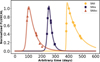 |
Fig. 1 Example of Bazin fits on three different types of SNe from the PLAsTiCC dataset, in the LSST-r filter: SNIbc (brown triangles), SNIa (blue crosses), and SNII (yellow circles). For each light curve, the flux is normalized by its maximum measured value. The time (horizontal axis) is arbitrarily shifted to display all three examples in a single frame. Error bars are included, but are contained within the points. |
2.2 Temperature
Despite being used to describe different types of transients, the Bazin function is most commonly applied on SNe. Consequently, we used a temperature evolution function coherent with SN classes. Using the SUpernova Generator And Reconstructor model (SUGAR; Léget et al. 2020), which is a SNIa spectral energy distribution model, we took a spectrum from −12 to 48 days since maximum brightness in B band with a step of 3 days. Each spectrum was fit with a blackbody function to obtain the temperature at a given time, effectively reconstructing the temperature evolution (Fig. 2). We visually inspected the results from a sigmoid-like fit (Eq. (4)) and confirmed that it is a good first approximation for the temperature behavior, but remains still relatively simple and general. Thus, we parameterized the temperature evolution as
 (4)
(4)
which is a four-parameter logistic function behaving as two flat curves linked by an exponential slope. Tmįn is the minimum temperature that the object will reach, ΔT describes the full amplitude of temperature, ksig corresponds to a characteristic timescale, and t0 is a reference time parameter that corresponds to the time at half of the slope. Preliminary results using independent t0 for Eqs. (3) and (4) often resulted in almost equally well fit values. Therefore, we assumed that t0 from both equations are equal and merged them into a single parameter. We used Eq. (4) to describe the temperature evolution in Eq. (1).
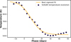 |
Fig. 2 Best logistic function fit of temperature evolution extrapolated from the SUGAR model. The data points have been computed by fitting blackbodies to the SNIa spectra from 3250 to 8650 Å at regular time intervals. The phase corresponds to the time since maximum brightness. |
Initial guess, lower and upper bounds of the parameters for the minimization step.
2.3 Feature extraction
As a preprocessing step, each light curve was normalized by the maximum flux measured in LSST-r passband (for the data described in Sect. 3) or ZTF-r (for the data described in Sect. 5), which ensures a more uniform dataset. Then, we fit the light curves and extract the resulting best-fit parameters. The minimization step was performed using the least-squares method from the IMINUIT Python library5 (James & Roos 1975). Table 1 summarizes the initial guesses and bounds of the parameters that were used at the minimization step (for the MONOCHROMATIC method, the same choices were applied to the relevant parameters). t0, trise, tfall, and ksig are expressed in days. Tmin and ΔT are expressed in kelvin. peak is the maximum measured flux over all filters. peak_time corresponds to the time of peak. We report an average run time of 120 ms per fit for the SNe from the PLAsTiCC dataset using the cuts described in Sect. 3.
When using the MONOCHROMATIC approach, we performed a Bazin fit (Eq. (3)) for each filter separately. Given the functional form, we extracted four parameters per passband. Additionally, we collected the least-squares loss of the fitting process as a feature for each passband. The r-band flux normalization factor computed previously was included as well. Therefore, we extracted nfeatures = 5npassbands + 1 features for each object.
In the context of the RAINBOW method, we performed a single fit of all the filters at the same time using Eq. (1), resulting in seven best-fit parameters. Additionally, we kept the least-square loss of the fitting process and the normalizing factor. Therefore, we extracted nine features for each object, independently of the dataset considered.
3 Data
We performed benchmark tests on data from the PLAsTiCC dataset (Hložek et al. 2020). PLAsTiCC was a classification challenge that took place in 2018, and whose goal was to mimic the data situation as expected from LSST.
Each astronomical source was represented by a noisy and inhomogeneously sampled light curve in six different filters6: u, g, r, i, z, and Y. The complete dataset consisted of around 3.5 million light curves, representing 17 classes that encompassed both transient and variable objects. In principle, RAINBOW could handle any number of passbands, but increasing the number of filters used in the analysis results in greater chances of objects being insufficiently sampled in at least one passband, which implies that this is not suited for the MONOCHROMATIC method and thus prevents a fair comparison of the two paradigms. Therefore, we chose to work with three passbands and discarded u, z and Y, for which the blackbody approximation of SN is least valid (Pierel et al. 2018). The superluminous supernovae (SLSN) and M-dwarf models used in the PLAsTiCC dataset explicitly used a blackbody SED. Consequently, using the RAINBOW method on SLSNe from this dataset results in an optimal color description.
We selected every well-populated transient types within PLAsTiCC, namely SNIa, SNII, SNIbc, SLSN, and TDEs. The first three SN types were used for all analyses, while TDE and SLSN were only added in the classification tests (Sect. 4.3) with the goal of increasing the complexity of the task. We required each passband to hold at least four photometric true detection points (see Kessler et al. 2019, Sect. 6.3 for a full explanation of true detection). This cut is imposed by the MONOCHROMATIC method based on the Bazin equation (Eq. (3)). It is the minimum requirement for the minimization to be reasonable and was therefore applied to both methods. The minimum requirement for RAINBOW (at least seven true detection points over all passbands) is always true if the previous requirement is verified. Furthermore, we required that the time of peak luminosity (defined as PEAKMJD inside the PLAsTiCC metadata) was included within the time span of the light curve.
We used only PLASTiCC data from the Wide Fast Deep (WFD) survey strategy. It represents most of the objects from the simulation and is less well sampled than the Deep Drilling Field (DDF) strategy, making it a perfect test case for sparsely sampled data. The requirements described above are very selective considering the cadence of the dataset, and only 0.4% of the SN classes passed the cuts. This highlights the importance of reducing the required number of points per band, which would increase the number of objects considered in the analysis. We performed feature extraction for objects within the WFD sample and stopped when we reached 1000 objects of each type or until we ran out of objects. Following this procedure, we built a database made of 1000 SNIa, 1000 SNII, 468 SNIbc, 1000 SLSN, and 372 TDE.
Additionally, we produced a second more challenging database using only the rising part of the light curves. We proceeded by removing all points after PEAKMJD, which corresponds either to the time of maximum flux in the B passband in the emitter frame for SNIa, or to the bolometric flux for the other transients7. We maintained the same feature extraction method as previously, including the requirement of the minimum number of points. This resulted in a smaller database containing 626 SNIa, 532 SNII, 317 Ibc, 616 SLSN, and 269 TDE.
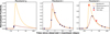 |
Fig. 3 Quality of the light-curve fit to a PLAsTiCC SNIa light curve. The red diamonds represent points that were randomly removed and were only used to compute the nRMSEo error. The fits were performed considering only points shown as dark blue circles. The error bars are displayed, but are contained within the points. |
4 Results
We evaluated the performance of RAINBOW through a comparison against the standard MONOCHROMATIC method. This analysis comprises both direct and indirect evaluations. The direct method consists of a measurement of the quality of the light-curve reconstruction (Sect. 4.1). However, since the reconstruction quality metric does not necessarily reflect the information loss, we also performed two additional indirect tests: the prediction of the peak time (Sect. 4.2), and two classification exercises (Sect. 4.3).
4.1 Quality of fit
This test was performed independently on all selected SNIa, SNII, and SNIbc following the method proposed in Demianenko et al. (2023). The light-curve time span was divided into 5-day-long bins. We randomly selected two bins containing at least one true detection point each, from which all photometric points were removed. This effectively resulted in two random 5-day-long gaps in the light curve. After this step, if enough points remained to fulfill the minimum requirement, they were submitted to the two feature extraction methods. The removed points were used to compute the agreement between the estimated light curve and the measured values. We used the normalized root mean squared error based on observed error (nRMSEo) as a quality metric,
![Mathematical equation: ${\rm{nRMSEo}} = \sqrt {{1 \over m}\sum\limits_i {\left[ {{{{{\left( {{y_i} - \mu \left( {{t_i}} \right)} \right)}^2}} \over {2_i^2}}} \right]} } $](/articles/aa/full_html/2024/03/aa48158-23/aa48158-23-eq5.png) (5)
(5)
where ti is the time of measurement, yi is the observed flux, ∈i is the observed flux error, µ(ti) is the estimated flux at the time ti, and m is the number of observations inside the test sample.
Figure 3 illustrates the procedure and the resulting fits on a given SNIa example for both methods. It highlights that RAINBoW is resilient to information loss. one point removed in the i-filter carries much information regarding the maximum flux of the object. In the i-filter, the MONOCHROMATIC method misses the peak observation by 20 days with half of the intensity, while RAINBOW exploits the information brought by the r passband and produces a more realistic light curve.
Table 2 displays the median nRMSEo error for the different classes of SNe. It also provides the 25/75 percentiles. The results are presented for each separate class of SN along with the global result (All SNe). In order to facilitate comparison, we estimated after visual inspection that an nRMSEo error below 7 can reliably be considered a correct fit for SN-like light curves (the theoretical perfect fit of this metric is  ). RAINBOW provides a better median error of 4.7 overall, against 5.6 for the MONOCHROMATIC method. The improvement in the fit quality is clear for SNIa and SNIbc, while both methods perform similarly for SNII.
We note that the 25 percentile of errors tends to be higher for the RAINBOW method. This means that the very best fits are more often produced by the MONOCHROMATIC method. This result is expected since good fits are associated with well-sampled data, and we know that the blackbody assumption is only a first-order approximation. Therefore, when many data points are available, it can act as a constraint on the fit. Conversely, the 75 percentiles show much lower error values of the RAINBOW method overall, which indicates that the method produces less extremely incorrect light curves than the MONOCHROMATIC method. This was confirmed by computing the mean nRMSEo error (less resilient to outliers), for which we obtained 8.8 and 13.1 for the RAINBOW and the MONOCHROMATIC method, respectively.
4.2 Peak time prediction
In this section, we consider a regression task aimed to estimate the time of maximum flux as an indirect approach to evaluate the quality of the light-curve reconstructions. PLAsTiCC metadata contain the value PEAKMJD corresponding to the time of the peak flux. It is defined by the time of maximum flux in the B Bessel passband in the source rest frame for SNIa (in that case, we used PLAsTiCC redshift metadata), or in received bolomet-ric flux for every other transient7. We predict this value using a direct and an indirect method.
The direct-prediction method highlights the versatility of RAINBOW. The 2D fit function (Eq. (1)) gives access to the flux in any passband at any time. Additionally, RAINBOW provides a direct estimate of the bolometric flux of the object. Therefore, in the case of SNIa, we can directly compute the time of maximum flux in the B passband even when no measurements were taken at this wavelength. For the other transients, we can use the bolometric flux explicitly encoded in the equation. In this analysis, we predicted the PEAKMJD for SNIa, SNII, and SNIbc.Figure 4 presents the distribution in the difference between the prediction and the reported peak time per class. We fit the distribution with a Gaussian to obtain a mean and a standard deviation. The method provides unbiased results for SNII. The SNIa and SNIbc predictions are biased around 3 days before and after the peak, respectively. While the bias exist, an error of 3 days constitutes a small error for a peak prediction of the considered SNe classes. The results show a small spread overall, especially for SNIa and SNII, with a standard deviation of 2.9 days.
This method has the advantage of offering a direct computation of the time of maximum, but it can only be computed for the RAINBOW method. The MONOCHROMATIC feature extraction procedure does not provide information about the bolometric or the B passband flux. For a fair comparison of the quality of prediction, we computed a second indirect metric using the scikit-learn linear regression8 algorithm trained on the features extracted from both methods.
We evaluated the performances on 100 iterations (Raschka 2018) of bootstrapping (Efron 1979), which is sufficient to produce robust results. Figure 5 displays histograms of all bootstrapping predictions combined for each SN class. Additionally, we fit a Gaussian to the distribution result of each bootstrapping iteration, from which we extracted the standard deviation and the mean. The Gaussians presented in Fig. 5 represent the mean Gaussian of the bootstrapping iterations. The colored area around the Gaussians represent a 1σ deviation of the bootstrapping standard deviation distribution.
The results show the excellent predictive power of the RAINBoW features for SNIa, with a mean of 0.8 and a standard deviation of 2.3 days (Fig. 5, top panel). The MONOCHROMATIC features resulted in a very wide distribution with a standard deviation of 8.9 days. In the case of SNII, both sets of features result in widely spread predictions. For this particular type, using a direct prediction provides a much better indicator for the time of the flux maximum. For SNIbc the results for the two methods are very similar, with a slight improvement in the standard deviation for the linear regression trained with the RAINBOW features.
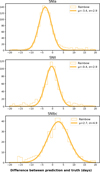 |
Fig. 4 Distribution per class of SNe of the difference between the RAINBOW prediction and the reported time of maximum as given within the PLAsTiCC metadata. The RAINBOW prediction is directly computed from the light-curve estimate using the definition of PLAsTiCC PEAKMJD. Additionally, a Gaussian was fit to the distributions to evaluate its mean and standard deviation. |
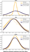 |
Fig. 5 Distribution per class of SNe of the difference between the prediction and true time of maximum as given within the PLAsTiCC metadata. The predictions have been computed based on linear regressor models trained with RAINBOW (yellow) and MONOCHROMATIC (dark blue) features. Additionally, a Gaussian was fit to the distributions to evaluate its mean and standard deviation. |
4.3 Classification
A common way to use features extracted from light curves is in ML classification tasks (e.g., Xu et al. 2023; Sánchez-Sáez et al. 2021). An informative set of features provides a good summary description of an object and can be used to distinguish several types of classes. We performed a multiclass classification exercise as a way to measure the relative information quality of the features extracted using the RAINBOW method compared to the those resulting from the MONOCHROMATIC procedure. A grid search over the max_features and max_depth hyperparame-ters led to no significant improvement of either model over the default hyperparameters. Therefore. we left all hyperparameters at default values to ensure a fair comparison. For the classification algorithm, we used the random forest implementation from the Sklearn library9 (Pedregosa et al. 2011). We decided to perform two classification challenges, one with the full light curves, and the other using only the rising part.
For the first exercise, we subsampled the database from Sect. 3 and built a balanced dataset of 300 light curves of each class (SNIa, SNII, SNIb, SLSN, and TDE), thus ensuring a uniform representation of the different light-curve shapes. We evaluated the results with 100 iterations of bootstrapping.
Figure 6 displays the differences in median confusion matrix between the RAINBOW features and the standard features. The overall median accuracy values are 88.4% and 81.9%, respectively (see Appendix B, Figs. B.1, and B.2 for the individual confusion matrices). The results clearly show that features extracted with the RAINBOW method enclose more discriminative information. Not only the overall accuracy is better, but every single type of transient is more accurately classified. We note that the long-lasting transients SNII, SLSN, and TDE, display the largest improvement over the MONOCHROMATIC method.
Figure 7 presents the importance of each RAINBOW feature in the classification process. The second and third most important features for separating the different classes are tfall and trise. They come from the bolometric function and are predictably key in the description of a transient type. The most relevant feature is Tmin, which describes the minimum temperature that the object will reach after the event. This underlines the importance of the blackbody approximation within the RAINBOW model.
In order to quantify the difference of the results between the two classifiers, we performed a corrected McNemar test as proposed in Yu & Liu (2003). From this test, we computed a χ2 that gives the degree of certainty with which we can reject the null hypotheses, that is, that resulting differences are due to random chance and that the two classifiers perform equally well.
We computed a 2 × 2 matrix (Table 3) that compared the two model predictions to each other (which should not be confused with a classical confusion matrix result from a given model). This matrix was computed at each bootstrapping step, and the table displays the average over the 100 iterations. The meaningful squares are the top right (TR) and bottom left (BL) since they displayed all the cases where the classifiers output different answers. From this we computed the χ2 metric as
 (6)
(6)
After the computation, we obtained a χ2 = 13, which in the case of one degree of freedom results in a p-value of 3 × 10⁻⁴. This result shows with a confidence higher than 3 σ that the resulting differences are not due to random chance.
Previous classification results displayed good performances of the RAINBOW method on complete light curves, but in some cases, an early classification on a still rising transient might be required in order to decide about a telescope follow-up (e.g., Leoni et al. 2022). Thus, we evaluated the RAINBOW method by repeating the classification exercise in this scenario. From the rising light-curve database described in Sect. 3, we randomly built a balanced dataset of 250 of each class (SNIa, SNII, SNIb, SLSN, and TDE). The number of objects per class must be reduced to 250 to maintain a balanced dataset. As previously, we applied 100 iterations of bootstrapping and used a random forest algorithm to build a classifier. Similarly to Sect. 4.3, we computed the differences in median confusion matrix between the RAINBOW and the MONOCHROMATIC features, as shown in Fig. 8. The overall median accuracies are 59.5% and 50.9%, respectively (see Appendix B, Figs. B.3 and B.4 for the individual confusion matrices). The results again show that RAINBOW features lead to a better classification of each type of rising transients. TDE display the largest difference with an accuracy improved by more than 19%. With the exception of SNII, all other rising SNe are clearly better disentangled using the rainbow features. The type SNII include SNII-P events that are characterized by a slowly decreasing plateau phase. In the case of rising light curves, we lose this determinant information, which could explain the decrease in the accuracy differences when compared to full SNII light-curve case.
Figure 9 presents the importance of each RAINBOW feature in the classification process of rising light curves. In this scenario, trise is the most important feature, which is coherent given the early classification challenge. Other features, including those related to temperature, provide second-order information and are all equally useful overall.
We also performed a McNemar test for this scenario. The average correct and incorrect classification of the two methods are shown in Table 4. Applying Eq. (6), we obtained a χ2 = 10.7, which is equivalent to a p-value of 1 × 10⁻³. The result is again statistically robust and leads to a confidence higher than 3 σ.
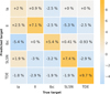 |
Fig. 6 Confusion matrix difference between the random forest classifiers trained on RAINBOW and MONOCHROMATIC features (normalized on precision). The dataset is composed of 300 light curves of each class (SNIa, SNII, SNIbc, SLSN, and TDE). The numbers represent the difference (RAINBOW – MONOCHROMATIC) in the median score of 100 iterations of bootstrapping. Individual confusion matrices for each method are given in Appendix B (Figs. B.1 and B.2). |
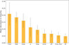 |
Fig. 7 Mean feature importance over 100 bootstrapping iterations of the random forest classifier trained with RAINBOW features. |
Mean contingency table of objects correctly and incorrectly classified by the random forest models trained with RAINBOW and standard features over 100 bootstrapping iterations.
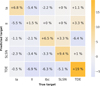 |
Fig. 8 Confusion matrix difference between the random forest classifiers trained on RAINBOW features and MONOCHROMATIC features (normalized on precision). The dataset is composed of 250 rising light curves of each class (SNIa, SNII, SNIbc, SLSN, and TDE). The numbers represent the difference (RAINBOW – MONOCHROMATIC) in the median score of 100 iterations of bootstrapping. Individual confusion matrices for each method are given in Appendix B (Figs. B.3 and B.4). |
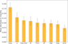 |
Fig. 9 Mean feature importance over 100 bootstrapping iterations of the random forest classifier trained with RAINBOW features from rising light curves. |
Mean contingency table of rising objects correctly and incorrectly classified by the random forest models trained with RAINBOW and standard features over 100 bootstrapping iteration.
5 Real data application
In this section, we demonstrate the capabilities of the method when applied to a real data multisurvey scenario, and compare it to the MONOCHROMATIC procedure. We used the Young Supernova Experiment Data Release 1 (YSE DR1, Aleo et al. 2023), which contains final photometry of 1975 transients observed by the Zwicky Transient Facility (ZTF, Bellm et al. 2019) gr and Pan-STARRS1 (PS1, Chambers et al. 2016) griz. YSE DR1 is the largest available low-redshift homogeneous multiband dataset of SNe, and thus provides the perfect testing ground for a variety of real objects. It encompasses SNe observations across vast timescales, magnitudes, and redshifts: those that last a few days to over a year, ranging in apparent magnitudes m = [12m, 22m], and span a redshift distribution up to z ~ 0.5.
While adding crucial deep photometry, the PS1 global cadence is well below that of ZTF, which makes an independent filter fit impossible in many cases due to insufficient number of photometric points. This implies that a traditional feature extraction step will result in a significant loss of objects. This issue can be addressed by considering PS1-gr and ZTF-gr as equivalent, effectively stacking the light curves. While this approximation is generally accurate, small discrepancies can be observed because of the differences in passband transmission profiles10,11 and the difference in photometric pipelines. Therefore, the rigorous approach is to consider the passbands independently. In this context and in the context of multisurvey analysis in general, RAINBOW offers the possibility to perform fits on all data available at once, without any passband approximation.
We compared RAINBOW and the standard method using the evaluation of the quality of the fit described in Sect. 4.1. We used all spectroscopically confirmed SNIa, SNII, and SNIbc, including nondetections, for a total of 254 SNe available in Zenodo12 (Aleo et al. 2022). Additionally, we manually added two nonde-tection points in the ZTF-gr passbands at −300 and −400 days before the measured maximum flux time. This provided a flux baseline that helps constrain the fit, especially when only the falling part of the light curve is available. We show results for two cases: first, where the dataset was entirely used to perform a RAINBOW fit (seven parameters per object); and second, where the combined PS1-gr and ZTF-gr light curves were fit independently with the MONOCHROMATIC method (eight parameters per object). Since PS1-i is poorly sampled (30% of the objects contain fewer than four detection points) and no ZTF-i band is available, we decided to restrict our test to gr passbands.
This dataset provides well-sampled light curves with 15 and 19 detection points on average in the g and r passbands from ZTF and PS1 combined, respectively. Since RAINBOW is particularly efficient at compensating the lack of information from poorly sampled passbands, we expect both methods to perform equally well in this scenario. Therefore, we compared the methods for different sampling levels. We created eight datasets by randomly sampling from 30% to 100% of the points in steps of 10%. In order to provide uncertainties, we performed this procedure ten times with different seeds. Since we still require a minimum number of points per passband (see Sect. 3), the datasets contained from 123 SNe for 30% sampling to 254 SNe for the complete sample on average. Figure 10 illustrates the fits on a SNII (SN 2020thx) sampled at 50%. We display the average median nRMSEo error (Eq. (5)) per sampling level in Fig. 11. The error bars correspond to one standard deviation of the median erroroverthe ten seeds. The areaofeach pointis proportional to the mean number of SNe in each sample. RAINBOW is clearly superior, especially in extreme situations when the number of points is severely limited. Both methods are equivalent in terms of predicting the light-curve profile when using 90% or more of the original number of points. This result indicates that the small additional information provided by PS-i together with the physical assumptions of the RAINBOW framework make a crucial difference on sparse transient datasets.
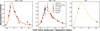 |
Fig. 10 Quality-of-fit evaluation process on a YSE DR1 SNII light curve (SN 2020thx). The red points were randomly removed and used to compute the nRMSEo error. The fits were performed only considering the dark points. |
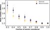 |
Fig. 11 Evolution of the median nRMSEo error for different sizes of the subsample of the YSE dataset. The error bars represent one standard deviation of the ten random subsamples. The data point surface is proportional to the mean number of SNe in the samples, from 123 for 30% to 25 for 100%. |
6 Conclusion
Estimating a continuous light-curve behavior from sparse and noisy photometric measurements is ofcrucial importance for the study of astronomical transients. When applied to large datasets, it can help us to understand the general behavior of under-represented classes, as well as extreme examples of the most well-studied classes (e.g., Sanders et al. 2015). Moreover, with the advent of large-scale sky surveys such as LSST, features from photometric light curves are used to feed ML classifiers, since they will be the sole information available for the majority of the observed transients (Hložek et al. 2020).
The RAINBOW framework presented here produces a continuous 2D surface in time and wavelength (Appendix A.1) even when the light curves are sparsely sampled in a number of different passbands. It starts by assuming that the thermal-electromagnetic behavior of the transient can be approximated by a blackbody, and it incorporates user-defined parametric functions representing the temperature evolution and bolometric light-curve behavior. As a result, it uses information in the available bands to inform the reconstruction in other wavelengths, providing a simple and robust framework for the estimation and feature extraction, which is especially suited when the data are sparse or spread across a set of passbands.
We used simulated data from PLAsTiCC to demonstrate the effectiveness of the method in a series of tests: goodness of fit (Sect. 4.1), estimation of the time of peak brightness (Sect. 4.2), and using the best-fit parameter values as input to machine-learning-based classifications (Sect. 4.3). In all these, we compared RAINBOW to the more traditional approach of fitting a parametric function independently to each passband (the MONOCHROMATIC method). The results show that RAINBOW outperforms or equals the results obtained from the traditional method, with the advantage of being applicable to significantly more sparse light curves.
Nevertheless, the method also inherits the drawbacks of the blackbody assumption, which may not be suitable for specific science cases. For example, the energy distribution of a supernova is far from being a blackbody in the ultraviolet and infrared spectrum (e.g., Faran et al. 2018). The RAINBOW method should be used in all wavelengths and epochs for which the blackbody assumption holds. This assumption was used as a first-order approximation for various types of objects, including super-novae, classical novae, tidal disruption events, and many others. The blackbody approximation might therefore be effective for a transient classification task across a wide range of classes, even when the specific class of the object remains unknown.
Caution should also be applied for very well sampled light curves. Even when the blackbody hypotheses is valid, it remains an approximation to physically describe the gaps in the data. In the case of high-cadence measurements, it acts as a constraint that can erase important information. Whenever a large number of data points is available, allowing the necessary number of parameters to be fit by independently fitting a parametric function to each passband will result in a better approximation. We demonstrated this issue using real data from YSE DR1 (Sect. 5). The results showed that RAINBOW provides significantly more informative reconstructions for a small number of observations.
In the tests presented here, we used a particular set of functions to represent the temperature and bolometric light-curve behavior, but these can be easily replaced by more suitable functions depending on the class of transients that is analysed13.
The blackbody spectrum approach presented in this paper can be generalized to any parametric SED model. For instance, power-law SEDs are commonly observed in various types of objects: those populating synchrotron emission (e.g., optical afterglows of gamma-ray bursts and UV emission of stellar flares), accretion disk outbursts (e.g., dwarf novae and active galaxy nuclei), and others. For a better performance of the ML pipelines, we suggest using multiple models based on different spectral parameter evolution laws while keeping the parameter bound ranges broad enough to cover objects of different astrophysical classes.
RAINBOW has been incorporated into a well-established feature extraction package14 (Malanchev et al. 2021) that is already used by three different community brokers: ANTARES (Matheson et al. 2021), AMPEL (Nordin et al. 2019), and Fink (Möller et al. 2021). Thus, it can be immediately used by the community to analyze the alert data.
In the context of modern astronomical surveys, not only the volume of data will pose an important challenge. The quality and complexity of the data gathered by new surveys will also evolve. LSST will push the limits of detection to even fainter magnitudes in six different passbands, but the majority of the survey strategy (wide-fast-deep) will probably consist of significantly sparse light curves for at least a few of the passbands (Lochner et al. 2018). In this context, RAINBOW represents an efficient option to enable modeling and analysis of multidimension light curves.
Acknowledgements
This work significantly benefited from 2 SNAD workshops: SNAD-V (https://snad.space/2022/), held in Clermont Ferrand - France, in 2022, and SNAD-VI (https://snad.space/2023/), held in Antalya -Turkey, in 2023. The reported study was funded by RFBR according to the research project no. 21-52-15024. The authors acknowledge the support by the Interdisciplinary Scientific and Educational School of Moscow University “Fundamental and Applied Space Research”. P.D.A. is supported by the Center for Astrophysical Surveys (CAPS) at the National Center for Supercomputing Applications (NCSA) as an Illinois Survey Science Graduate Fellow.
Appendix A Surface plot
Figure A.1 illustrates the shape of a 2D surface built from real light curves from SN2020thx using the RAINBOW approach.
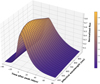 |
Fig. A.1 Surface plot representation of a RAINBOW fit of a SNII (SN 2020thx) light curve. Representations per passband of the same object with the data points are displayed in Figure 10. |
Appendix B Rainbow classification confusion matrices
Classification confusion matrix of random forest models trained on RAINBOW (Figures B.1 and B.3) and MONOCHROMATIC features (Figures B.2 and B.4).
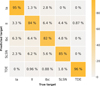 |
Fig. B.1 Full light-curve scenario. Confusion matrix normalized on the precision of the random forest classifier trained on RAINBOW features. The dataset is composed of 300 light curves of each class (SNIa, SNII, SNIbc, SLSN, and TDE). The numbers represent the median score of 100 iterations of bootstrapping. These results were used to construct those shown in Figure 6. |
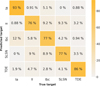 |
Fig. B.2 Full light-curve scenario. Confusion matrix normalized on the precision of the random forest classifier trained on MONOCHROMATIC features. The dataset is composed of 300 light curves of each class (SNIa, SNII, SNIbc, SLSN, and TDE). The numbers represent the median score of 100 iterations of bootstrapping. These results were used to construct those shown in Figure 6. |
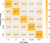 |
Fig. B.3 Rising light-curve scenario. Confusion matrix normalized on the precision of the random forest classifier trained on RAINBOW features. The dataset is composed of 250 light curves of each class (SNIa, SNII, SNIbc, SLSN, and TDE). The numbers represent the median score of 100 iterations of bootstrapping. These results were used to construct those shown in Figure 8. |
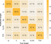 |
Fig. B.4 Rising light-curve scenario. Confusion matrix normalized on the precision of the random forest classifier trained on MONOCHROMATIC features. The dataset is composed of 250 light curves of each class (SNIa, SNII, SNIbc, SLSN, and TDE). The numbers represent the median score of 100 iterations of bootstrapping. These results were used to construct those shown in Figure 8. |
References
- Aleo, P. D., Malanchev, K., Sharief, S. N., et al. 2022, https://doi.org/10.5281/zenodo.7317476 [Google Scholar]
- Aleo, P. D., Malanchev, K., Sharief, S., et al. 2023, ApJS, 266, 9 [NASA ADS] [CrossRef] [Google Scholar]
- Bazin, G., Palanque-Delabrouille, N., Rich, J., et al. 2009, A&A, 499, 653 [NASA ADS] [CrossRef] [EDP Sciences] [Google Scholar]
- Bellm, E. C., Kulkarni, S. R., Graham, M. J., et al. 2019, PASP, 131, 018002 [Google Scholar]
- Boone, K. 2019, AJ, 158, 257 [NASA ADS] [CrossRef] [Google Scholar]
- Cannizzaro, G., Jonker, P. G., & Mata-Sánchez, D. 2021, ApJ, 909, 159 [NASA ADS] [CrossRef] [Google Scholar]
- Chambers, K. C., Magnier, E. A., Metcalfe, N., et al. 2016, arXiv e-prints [arXiv:1612.05560] [Google Scholar]
- Corsi, A., Ho, A. Y. Q., Cenko, S. B., et al. 2023, ApJ, 953, 179 [CrossRef] [Google Scholar]
- Deckers, M., Graur, O., Maguire, K., et al. 2023, MNRAS, 521, 4414 [NASA ADS] [CrossRef] [Google Scholar]
- Demianenko, M., Samorodova, E., Sysak, M., et al. 2023, J. Phys. Conf. Ser., 2438, 012128 [NASA ADS] [CrossRef] [Google Scholar]
- Desai, D. D., Ashall, C., Shappee, B. J., et al. 2023, MNRAS, 524, 767 [CrossRef] [Google Scholar]
- Efron, B. 1979, Ann. Stat., 7, 1 [Google Scholar]
- Faran, T., Nakar, E., & Poznanski, D. 2018, MNRAS, 473, 513 [NASA ADS] [CrossRef] [Google Scholar]
- Fulton, M. D., Smartt, S. J., Rhodes, L., et al. 2023, ApJ, 946, L22 [NASA ADS] [CrossRef] [Google Scholar]
- Hložek, R., Ponder, K. A., Malz, A. I., et al. 2020, arXiv e-prints [arXiv:2012.12392] [Google Scholar]
- Ishida, E. E. O. 2019, Nat. Astron., 3, 680 [NASA ADS] [CrossRef] [Google Scholar]
- Ishida, E. E. O., Beck, R., González-Gaitán, S., etal. 2019, MNRAS, 483, 2 [Google Scholar]
- Ivezić, Ž., Kahn, S. M., Tyson, J. A., et al. 2019, ApJ, 873, 111 [Google Scholar]
- James, F., & Roos, M. 1975, Comput. Phys. Commun., 10, 343 [Google Scholar]
- Karpenka, N. V., Feroz, F., & Hobson, M. P. 2013, MNRAS, 429, 1278 [NASA ADS] [CrossRef] [Google Scholar]
- Kelly, P. L., Rodney, S., Treu, T., et al. 2023, ApJ, 948, 93 [NASA ADS] [CrossRef] [Google Scholar]
- Kessler, R., Narayan, G., Avelino, A., et al. 2019, PASP, 131, 094501 [NASA ADS] [CrossRef] [Google Scholar]
- Kornilov, M. V., Semenikhin, T. A., & Pruzhinskaya, M. V. 2023, MNRAS, 526, 1822 [NASA ADS] [CrossRef] [Google Scholar]
- La Mura, G., Berton, M., Chen, S., et al. 2017, Front. Astron. Space Sci., 4 [CrossRef] [Google Scholar]
- Léget, P.-F., Gangler, E., Mondon, F., et al. 2020, A&A, 636, A46 [NASA ADS] [CrossRef] [EDP Sciences] [Google Scholar]
- Leoni, M., Ishida, E. E. O., Peloton, J., & Moller, A. 2022, A&A, 663, A13 [NASA ADS] [CrossRef] [EDP Sciences] [Google Scholar]
- Lochner, M., Scolnic, D. M., Awan, H., et al. 2018, arXiv e-prints [arXiv:1012.00515] [Google Scholar]
- Malanchev, K. L., Pruzhinskaya, M. V., Korolev, V. S., et al. 2021, MNRAS, 502, 5147 [Google Scholar]
- Matheson, T., Stubens, C., Wolf, N., et al. 2021, AJ, 161, 107 [NASA ADS] [CrossRef] [Google Scholar]
- McCully, C., Jha, S. W., Scalzo, R. A., et al. 2022, ApJ, 925, 138 [NASA ADS] [CrossRef] [Google Scholar]
- Möller, A., Peloton, J., Ishida, E. E. O., et al. 2021, MNRAS, 501, 3272 [CrossRef] [Google Scholar]
- Muthukrishna, D. 2022, in Am. Astron. Soc. Meeting Abstracts, 54, 215.06 [Google Scholar]
- Nordin, J., Brinnel, V., van Santen, J., et al. 2019, A&A, 631, A147 [NASA ADS] [CrossRef] [EDP Sciences] [Google Scholar]
- Nyholm, A., Sollerman, J., Tartaglia, L., et al. 2020, A&A, 637, A73 [NASA ADS] [CrossRef] [EDP Sciences] [Google Scholar]
- Padovani, P., Alexander, D. M., Assef, R. J., et al. 2017, A&A Rev., 25, 2 [NASA ADS] [CrossRef] [Google Scholar]
- Pedregosa, F., Varoquaux, G., Gramfort, A., et al. 2011, J. Mach. Learn. Res., 12, 2825 [Google Scholar]
- Pierel, J. D. R., Rodney, S., Avelino, A., et al. 2018, PASP, 130, 114504 [NASA ADS] [CrossRef] [Google Scholar]
- Poudel, M., Sarode, R. P., Watanobe, Y., Mozgovoy, M., & Bhalla, S. 2022, Appl. Sci., 12 [Google Scholar]
- Raschka, S. 2018, arXiv e-prints [arXiv: 1811.12808] [Google Scholar]
- Rodrigo, C., Solano, E., & Bayo, A. 2012, SVO Filter Profile Service Version 1.0, IVOA Working Draft 15 October 2012 [CrossRef] [Google Scholar]
- Sanders, N. E., Soderberg, A. M., Gezari, S., et al. 2015, ApJ, 799, 208 [NASA ADS] [CrossRef] [Google Scholar]
- Sánchez-Sáez, P., Reyes, I., Valenzuela, C., et al. 2021, AJ, 161, 141 [CrossRef] [Google Scholar]
- Villar, V. A., Berger, E., Miller, G., et al. 2019, ApJ, 884, 83 [NASA ADS] [CrossRef] [Google Scholar]
- Xu, Q., Shen, S., de Souza, R. S., et al. 2023, MNRAS, 526, 6391 [NASA ADS] [CrossRef] [Google Scholar]
- Yang, S., & Sollerman, J. 2023, ApJS, 269, 40 [NASA ADS] [CrossRef] [Google Scholar]
- Yu, L., & Liu, H. 2003, in Proceedings, Twentieth International Conference on Machine Learning, 2, 856 [Google Scholar]
- Zheng, W.,& Filippenko, A. V. 2017, ApJ, 838, L4 [CrossRef] [Google Scholar]
Richard Kessler, priv. comm.
A completely data driven option for the bolometric light-curve behavior based on symbolic regression is currently under development and will be the focus of a follow-up work (Russeil et al., in prep.).
All Tables
Initial guess, lower and upper bounds of the parameters for the minimization step.
Mean contingency table of objects correctly and incorrectly classified by the random forest models trained with RAINBOW and standard features over 100 bootstrapping iterations.
Mean contingency table of rising objects correctly and incorrectly classified by the random forest models trained with RAINBOW and standard features over 100 bootstrapping iteration.
All Figures
|
Fig. 1 Example of Bazin fits on three different types of SNe from the PLAsTiCC dataset, in the LSST-r filter: SNIbc (brown triangles), SNIa (blue crosses), and SNII (yellow circles). For each light curve, the flux is normalized by its maximum measured value. The time (horizontal axis) is arbitrarily shifted to display all three examples in a single frame. Error bars are included, but are contained within the points. |
| In the text | |
|
Fig. 2 Best logistic function fit of temperature evolution extrapolated from the SUGAR model. The data points have been computed by fitting blackbodies to the SNIa spectra from 3250 to 8650 Å at regular time intervals. The phase corresponds to the time since maximum brightness. |
| In the text | |
|
Fig. 3 Quality of the light-curve fit to a PLAsTiCC SNIa light curve. The red diamonds represent points that were randomly removed and were only used to compute the nRMSEo error. The fits were performed considering only points shown as dark blue circles. The error bars are displayed, but are contained within the points. |
| In the text | |
|
Fig. 4 Distribution per class of SNe of the difference between the RAINBOW prediction and the reported time of maximum as given within the PLAsTiCC metadata. The RAINBOW prediction is directly computed from the light-curve estimate using the definition of PLAsTiCC PEAKMJD. Additionally, a Gaussian was fit to the distributions to evaluate its mean and standard deviation. |
| In the text | |
|
Fig. 5 Distribution per class of SNe of the difference between the prediction and true time of maximum as given within the PLAsTiCC metadata. The predictions have been computed based on linear regressor models trained with RAINBOW (yellow) and MONOCHROMATIC (dark blue) features. Additionally, a Gaussian was fit to the distributions to evaluate its mean and standard deviation. |
| In the text | |
|
Fig. 6 Confusion matrix difference between the random forest classifiers trained on RAINBOW and MONOCHROMATIC features (normalized on precision). The dataset is composed of 300 light curves of each class (SNIa, SNII, SNIbc, SLSN, and TDE). The numbers represent the difference (RAINBOW – MONOCHROMATIC) in the median score of 100 iterations of bootstrapping. Individual confusion matrices for each method are given in Appendix B (Figs. B.1 and B.2). |
| In the text | |
|
Fig. 7 Mean feature importance over 100 bootstrapping iterations of the random forest classifier trained with RAINBOW features. |
| In the text | |
|
Fig. 8 Confusion matrix difference between the random forest classifiers trained on RAINBOW features and MONOCHROMATIC features (normalized on precision). The dataset is composed of 250 rising light curves of each class (SNIa, SNII, SNIbc, SLSN, and TDE). The numbers represent the difference (RAINBOW – MONOCHROMATIC) in the median score of 100 iterations of bootstrapping. Individual confusion matrices for each method are given in Appendix B (Figs. B.3 and B.4). |
| In the text | |
|
Fig. 9 Mean feature importance over 100 bootstrapping iterations of the random forest classifier trained with RAINBOW features from rising light curves. |
| In the text | |
|
Fig. 10 Quality-of-fit evaluation process on a YSE DR1 SNII light curve (SN 2020thx). The red points were randomly removed and used to compute the nRMSEo error. The fits were performed only considering the dark points. |
| In the text | |
|
Fig. 11 Evolution of the median nRMSEo error for different sizes of the subsample of the YSE dataset. The error bars represent one standard deviation of the ten random subsamples. The data point surface is proportional to the mean number of SNe in the samples, from 123 for 30% to 25 for 100%. |
| In the text | |
|
Fig. A.1 Surface plot representation of a RAINBOW fit of a SNII (SN 2020thx) light curve. Representations per passband of the same object with the data points are displayed in Figure 10. |
| In the text | |
|
Fig. B.1 Full light-curve scenario. Confusion matrix normalized on the precision of the random forest classifier trained on RAINBOW features. The dataset is composed of 300 light curves of each class (SNIa, SNII, SNIbc, SLSN, and TDE). The numbers represent the median score of 100 iterations of bootstrapping. These results were used to construct those shown in Figure 6. |
| In the text | |
|
Fig. B.2 Full light-curve scenario. Confusion matrix normalized on the precision of the random forest classifier trained on MONOCHROMATIC features. The dataset is composed of 300 light curves of each class (SNIa, SNII, SNIbc, SLSN, and TDE). The numbers represent the median score of 100 iterations of bootstrapping. These results were used to construct those shown in Figure 6. |
| In the text | |
|
Fig. B.3 Rising light-curve scenario. Confusion matrix normalized on the precision of the random forest classifier trained on RAINBOW features. The dataset is composed of 250 light curves of each class (SNIa, SNII, SNIbc, SLSN, and TDE). The numbers represent the median score of 100 iterations of bootstrapping. These results were used to construct those shown in Figure 8. |
| In the text | |
|
Fig. B.4 Rising light-curve scenario. Confusion matrix normalized on the precision of the random forest classifier trained on MONOCHROMATIC features. The dataset is composed of 250 light curves of each class (SNIa, SNII, SNIbc, SLSN, and TDE). The numbers represent the median score of 100 iterations of bootstrapping. These results were used to construct those shown in Figure 8. |
| In the text | |
Current usage metrics show cumulative count of Article Views (full-text article views including HTML views, PDF and ePub downloads, according to the available data) and Abstracts Views on Vision4Press platform.
Data correspond to usage on the plateform after 2015. The current usage metrics is available 48-96 hours after online publication and is updated daily on week days.
Initial download of the metrics may take a while.