| Issue |
A&A
Volume 683, March 2024
|
|
|---|---|---|
| Article Number | A121 | |
| Number of page(s) | 10 | |
| Section | Galactic structure, stellar clusters and populations | |
| DOI | https://doi.org/10.1051/0004-6361/202347603 | |
| Published online | 13 March 2024 | |
Galactic archaeology with [Mg/Mn] versus [Al/Fe] abundance ratios
Uncertainties and caveats
1
Dipartimento di Fisica, Sezione di Astronomia, Università di Trieste, Via G. B. Tiepolo 11, 34143 Trieste, Italy
2
INAF – Osservatorio Astronomico di Trieste, via G.B. Tiepolo 11, 34131 Trieste, Italy
e-mail: This email address is being protected from spambots. You need JavaScript enabled to view it.
3
INFN – Sezione di Trieste, via Valerio 2, 34134 Trieste, Italy
Received:
29
July
2023
Accepted:
9
November
2023
Abstract
Context. The diagram depicting the abundance ratios [Mg/Mn] versus [Al/Fe] has gained significant attention in recent literature as a valuable tool for exploring fundamental aspects of the evolution of the Milky Way (MW) and the nearby dwarf galaxies. In particular, this combination of elements is supposed to be highly sensitive to the history of star formation, unveiled by the imprints left on those abundances. Unfortunately, a complete discussion on the uncertainties associated with these nuclei is still missing, making it difficult to know how reliable the associated results are.
Aims. In this work, we aim to analyse, by means of detailed chemical evolution models, the uncertainties related to the nucleosynthesis of Mg, Al, Mn, and Fe to show how different yield prescriptions can substantially affect the trends in the [Mg/Mn] versus [Al/Fe] plane. In fact, if different nucleosynthesis assumptions produce conflicting results, then the [Mg/Mn] versus [Al/Fe] diagram does not represent a strong diagnostic for the star formation history (SFH) of a galaxy.
Methods. We discuss the results on the [Mg/Mn] versus [Al/Fe] diagram, as predicted by several MW and Large Magellanic Cloud (LMC) chemical evolution models adopting different nucleosynthesis prescriptions.
Results. The results show that the literature nucleosynthesis prescriptions require some corrective factors to reproduce the APOGEE DR17 abundances of Mg, Al, and Mn in the MW and that the same factors can also improve the results for the LMC. In particular, we show that by modifying the massive star yields of Mg and Al, the behaviour of the [Mg/Mn] versus [Al/Fe] plot changes substantially.
Conclusions. In conclusion, by changing the chemical yields within their error bars, one obtains trends that differ significantly, making it very difficult to draw any reliable conclusion on the SFH of galaxies. The proposed diagram is therefore very uncertain from a theoretical point of view, and it could represent a good diagnostic for star formation, only if the uncertainties on the nucleosynthesis of the above-mentioned elements (Mg, Mn, Al, and Fe) could be reduced by future stellar calculations.
Key words: astrochemistry / stars: abundances / Galaxy: abundances / Galaxy: evolution / galaxies: dwarf / Local Group
© The Authors 2024
 Open Access article, published by EDP Sciences, under the terms of the Creative Commons Attribution License (https://creativecommons.org/licenses/by/4.0), which permits unrestricted use, distribution, and reproduction in any medium, provided the original work is properly cited.
This article is published in open access under the Subscribe to Open model. This email address is being protected from spambots. You need JavaScript enabled to view it. to support open access publication.
1. Introduction
In a recent paper, Fernandes et al. (2023) compared the [Mg/Mn] versus [Al/Fe] relation for the stars of Gaia-Enceladus with those of several dwarf satellite galaxies of the Milky Way (MW), including the Large Magellanic Cloud (LMC) and the Small Magellanic Cloud (SMC), in order to establish if the stars in the Galactic halo were accreted or formed in situ. The above relation, in fact, is different for different SFHs, typical of different galactic systems that could have been the building blocks of the halo.
Galaxy mergers were common in the early Universe, and in recent years remnants of merging activity of the MW have been identified in several stellar streams. Moreover, the discovery of Gaia-Enceladus (Helmi et al. 2018) has suggested that a major merger occurred roughly 10 Gyr ago (Helmi et al. 2018; Montalbán et al. 2021) in the Galactic halo. The proposed [Mg/Mn] versus [Al/Fe] relation (Hawkins et al. 2015) can in principle discriminate between different star formation rates (SFRs). This is due to the different production timescales of the elements involved: Mn is produced with long time delays by Type Ia Supernovae (SNe Ia), which also contribute to the bulk of the Fe production, whereas massive stars (core-collapse supernovae; CC-SNe) produce Mg, Al and a small fraction of Fe. The data adopted by Fernandes et al. (2023) belong to the DR17 of the APOGEE Survey-2 (Majewski et al. 2017; Ahumada et al. 2020; Abdurro’uf et al. 2022). In the observational diagram, the stellar systems formed by means of an intense burst of star formation are expected to occupy a particular region with high [Mg/Mn] at high [Al/Fe], while objects that evolved with a mild SFR, such as dwarf spheroidals, show a lower [Mg/Mn] at low [Al/Fe]. Several observational investigations have indeed revealed a significant number of kinematically identified accreted stellar populations in the MW clumps, in the same region of the above-mentioned chemical plane (i.e. Feuillet et al. 2021; Perottoni et al. 2022; Horta et al. 2023; Feltzing & Feuillet 2023). Therefore, this diagram allows us to better distinguish the stars formed in situ from those accreted than using the classical [α/Fe] versus [Fe/H] ratios, which are very similar in all systems at low metallicity ([Fe/H]), due to the dominance of the enrichment by CC-SNe at early times (Spitoni et al. 2016). In fact, these [α/Fe] ratios observed in dwarf spheroidal galaxies (dSphs) and ultra-faint dwarf galaxies (UfDs) can coincide with those of halo stars at extremely low metallicities, while they diverge towards higher metallicities (Das et al. 2020).
The choice of the [Mg/Mn] ratio is to highlight the α-poor population better than [Mg/Fe] does, since Mn is a better tracer of SNe Ia. It should be noted that Spitoni et al. (2016) suggested adopting the [Ba/Fe] ratio as a discriminant of accreted stars instead of the [α/Fe] one, since Ba is mainly an s-process element produced by low-mass stars, and this ratio can be quite different in different star formation environments, especially at low metallicities. The same technique was also proposed from the observational point of view by Tolstoy et al. (2009) and references therein, where the ratio [Be/Fe] is presented in the case of four different dwarf spheroidals that show different behaviour due to the SFH of the environment under analysis.
In this article, we show that the theoretical [Mg/Mn] versus [Al/Fe] relation is strongly model dependent, and we highlight how different chemical evolution models can provide different solutions, thus suggesting caution should be taken when adopting such a tool. In any case, this should be combined with dynamical information, such as eccentricity, an energy-angular momentum relation, radial action-angular momentum, and action diamond (i.e. Myeong et al. 2019; Gaia Collaboration 2023; Carrillo et al. 2024), before drawing firm conclusions.
In Sect. 2, we present chemical models for the MW and for the LMC. In Sect. 3, the observational samples used in our analysis are described. In Sect. 4, we show our results. Finally, in Sect. 5, we critically discuss our results and draw conclusions. In particular, we discuss the role of the initial mass function (IMF) and the stellar yields on the results. The IMF has been derived only for the MW, so for the satellites of the Galaxy, we can only guess the best one that reproduces the observed features. Concerning the yields, large uncertainties are still present in the yields of Mn and Al.
2. Chemical evolution models for the MW and LMC
In this work, we considered models of Vasini et al. (2022, 2023), respectively, as reference models for the MW and for the LMC, and we label them as REF MW and REF LMC models. We also introduce NEW MW and NEW LMC models where we considered additional corrective factors on the nucleosynthesis yields, while keeping the other parameters the same. In addition, we combined some reference yields with some corrected ones in the MIX MW and MIX LMC models (see Sect. 4.2). Moreover, we also tested three additional MW models with different IMF, nucleosynthesis, and wind prescriptions. We present the model parameters in Table 1. In Sects. 2.1 and 2.2, we show all the prescriptions for the models, except the nucleosynthesis assumptions, which are presented in Sect. 2.3.
Parameters of the five MW and two LMC models tested (indicated in the first column).
2.1. The MW discs
We adopted the model of Vasini et al. (2022, where a more extensive description can be found) as a reference for studying the evolution of [Mg/Mn] versus [Al/Fe] abundance ratios in the MW disc components in the solar neighbourhood. This model, originally proposed by Chiappini et al. (1997, 2001) and later refined by Romano & Matteucci (2003), Grisoni et al. (2018), and Spitoni et al. (2019), is known as the two-infall model. The main chemical evolution equation on which the model is based accounts for the chemical enrichment and depletion of the gas:
 (1)
(1)
Here, Xi(t) and ψ(t) are the abundance by mass of element i and the SFR, respectively; Ri(t) is the rate at which the element i is restored into the interstellar medium (ISM); A(t) is the infall rate, and Xi, A(t) is the abundance of the element i in the infalling gas. This model traces the evolution of both the thick and thin discs; the thin disc is divided into concentric annuli 2 kpc wide, without exchange of matter. The thick disc is instead considered as a one-zone. It should be noted that in this paper we performed all the calculations in the solar neighbourhood (the annular area centred at 8 kpc from the Galactic centre). The formation process involves two distinct gas infall episodes, both following an exponential law. The first accretion event, characterised by a relatively short timescale (τT = 0.7 Gyr), leads to the formation of the thick disc. Subsequently, the second accretion event, with a delay from the first one of 1 Gyr, contributes to the formation of the thin disc, which takes place over significantly longer timescales. In particular, it is usually assumed that the thin disk formation timescale depends on the galactocentric distance, so that an ‘inside out’ scenario (Matteucci & Francois 1989) can be reproduced. This dependence follows the τD(R) = 1.033 ⋅ (R/kpc)−1.267 Gyr law, as shown by Chiappini et al. (2001).
The SFR is the Kennicutt (1998) law
 (2)
(2)
where ν is the star formation efficiency (fixed at the values of νT = 2 Gyr−1 and νD = 1 Gyr−1 for the thick and thin disc phases, respectively), σg is the surface gas density, and k = 1.5. In Fig. 1, we show the SFH of the MW for the solar neighbourhood (red line) compared to the measured present day as suggested by Prantzos et al. (2018; in the range 0.2–0.5 M⊙ yr−1, vertical orange line). In particular, we predict a present day value in the solar neighbourhood of ∼0.3 M⊙ yr−1. For the IMF, we used that of Kroupa et al. (1993, which is constant in time). The model accounts for the chemical contribution by SNII, Ib, Ic, Ia, as well as novae. The rate for the explosions of these stars are the same as those used in Vasini et al. (2022).
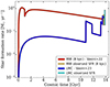 |
Fig. 1. SFHs predicted by Vasini et al. (2022, 2023) and used in the paper. For the MW (red line), the Kennicutt (1998) law with exponent k = 1.5 was adopted, and the temporal evolution of the star formation at the solar ring (8 kpc) is compared with the present-day observed SFR (vertical yellow line, data taken from Prantzos et al. 2018). For the LMC (blue line) we assumed a linear Kennicutt (1998) law with a variable efficiency to reproduce the Harris & Zaritsky (2009) SFR. We compared it with the observation at the present time by Harris & Zaritsky (2009) itself (vertical cyan line). |
2.2. The LMC
To study the chemical evolution of the LMC, we adopted the prescriptions of Model 3 presented in Vasini et al. (2023). The evolution of the abundances in the gas is described by Eq. (1) with the term −Xi(t)Wi(t) added on the right side of the expression. This accounts for the depletion of gas due to the galactic wind. The wind depends on the SFR ψ(t) through the mass loading factor ωi, whose value is reported in Table 1. In particular, the wind rate for the element i is
 (3)
(3)
The chemical evolution model of the LMC is a one-zone model based on a single infall law, an SFR with a linear Kennicutt (1998) law (k = 1), and a variable efficiency ν so as to reproduce the recent bursts studied by Harris & Zaritsky (2009). This irregular behaviour of the SFR is typical of the structures identified as dwarf irregular galaxies, as the LMC is traditionally classified. This SFH is shown in Fig. 1 (blue line) compared to the measurements by Harris & Zaritsky (2009) at the present time (within the interval 0.2–0.8 M⊙ yr−1, vertical cyan line). We predict a present time SFR of ∼0.4 M⊙ yr−1, which is compatible with the observed range.
2.3. Nucleosynthesis prescriptions
From now on, we refer to models REF MW and REF LMC when the nucleosynthesis prescription from Vasini et al. (2022, 2023) have been considered, which in turn were taken from Model 15 by Romano et al. (2010). In particular, we adopted Karakas (2010) for the nucleosynthesis in AGB stars, Kobayashi et al. (2006) for massive stars, Iwamoto et al. (1999) for SNIa, and José & Hernanz (1998) for nova systems.
On the other hand, models NEW MW and NEW LMC are based on the same yields, but with additional correction factors tailored to fit the abundance patterns of Mg, Al, and Mn in the MW, as explained in Sect. 4.1. We also computed a MIX MW model and a MIX LMC model with the combined prescriptions from the other models. The corrections are all listed in Table 2 and 3, where the first column indicates the element analysed, whereas the second, the third and the fourth are dedicated to Low-Intermediate Mass Stars, Massive stars and SNIa, respectively. The corrections listed are chosen to fit the MW APOGEE DR17 data and are applied to the yields adopted (whose reference is indicated in the first row as a reminder). The only exception is the Mn case, that we corrected as suggested by Cescutti et al. (2008), who introduced a metal dependency on the yields of this element. Then, in the model MW CL04 we performed a test using nucleosynthesis prescriptions identical to those employed by the chemical evolution models proposed by Andrews et al. (2017). In the same way, we performed two more tests with the K01 MW and WIND MW models, assuming the IMF and the wind prescriptions proposed by Andrews et al. (2017), respectively. These prescriptions were chosen since they are the reference ones in the paper by Fernandes et al. (2023).
Modified nucleosynthesis yields.
Yield correction adopted in MIX MW model and MIX LMC model.
3. Observational data
We compared our model predictions in the [Mg/Mn] versus [Al/Fe] abundance space for the MW and LMC with APOGEE-2 DR17 data as selected by Fernandes et al. (2023). The samples discarded unreliable parameters using the STARFLAG or ASPCAPFLAG=BAD indicators (see Holtzman et al. 2015 for definitions). Only red giant stars were considered by imposing the following conditions: stellar effective temperatures (Teff) ranging from 3750 to 5500 K and surface gravity log(g) < 3.0 dex.
The APOGEE stars of the MW were selected using orbital parameters in the integral of motion considering circular and prograde orbits: Lz > 0, eccentricity < 0.3, S/N > 70. As in Fernandes et al. (2023), we do not impose any condition on the galactocentric distances. In fact, model predictions in the solar vicinity (see Sect. 2.1) should represent the average behaviour of the whole MW disc well. They considered bright and faint red giant branch (RGB) stellar populations. In their Table 2, they summarised the LMC member selection indicating the sky position, projected distance on the sky, Gaia proper motions, radial velocities, and magnitudes. This selection mimics that proposed by Nidever et al. (2020), where Table 1 lists the APOGEE MC Fields.
4. Results
In this section, we present model results obtained for the MW and the LMC. First, in Sect. 4.1, we show the plots for the single abundances ([Mg/Fe], [Al/Fe], and [Mn/Fe]) for the MW and then the trends in the [Mg/Mn] versus [Al/Fe] plane in Sect. 4.2. In Sects. 4.3 and 4.4, we show the abundances and the [Mg/Mn] versus [Al/Fe] trends for the LMC, respectively. Finally, in Sect. 4.5, we describe how we tested the effects of adopting the nucleosynthesis prescriptions adopted by Andrews et al. (2017) on the chemical evolution of the MW discs.
4.1. MW: [Mg/Fe], [Al/Fe], and [Mn/Fe]
In Fig. 2, we compare the abundances of Mg, Al, and Mn for the MW that we predicted adopting the REF MW model (black lines) and the NEW MW model (white lines), with the APOGEE DR17 data. In the left panel, we note that the REF MW model underestimates Mg throughout the whole [Fe/H] range, which is a quite common feature among many sets of yields for this element (e.g. François et al. 2004; Romano et al. 2010; Prantzos et al. 2018; Lian et al. 2020). The underestimation is particularly pronounced for [Fe/H] ≳ − 0.5 dex, and it becomes larger towards the solar metallicity. To fix this behaviour, we can add corrections to slightly increase the Mg production, especially at the latest stages of the MW evolution. In the middle panel, REF MW model also shows an underestimation for Al. The data show a trend that is quite high at low metallicities ([Al/Fe] ∼ 0.25 dex) and then decreases as long as we go towards the solar value. Therefore, the Al yield should be increased at low [Fe/H] and then decreased. In the right panel, we present the Mn abundance. The REF MW model is quite compatible with the range of [Mn/Fe] across the [Fe/H] range spanned by the observations, although the shape of the trend is not that of the running median. In this case, the NEW MW model adopts a yield correction that was introduced by Cescutti et al. (2008) with a metallicity dependence, as shown in Table 2. This correction actually does not work as well as the original prescriptions, but it is worth also investigating the [Mg/Mn] versus [Al/Fe] plane.
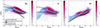 |
Fig. 2. Abundance ratios of the three elements involved. The data are from APOGEE DR17 and are binned and colour-coded according to the data density in each bin. The blue line represents the running median, computed assuming a bin size of 0.1 dex and an overlap of 0.025 dex, and the blue shaded area represents the related standard deviation. Left panel: [Mg/Fe] in the MW as predicted by REF MW model (black line) and by NEW MW model (white line) compared to APOGEE data. Middle panel: [Al/Fe] MW abundance for both models (same colour-coding as left panel). Right panel: [Mn/Fe] abundance for REF MW and NEW MW models (same colour-coding). |
Moreover, since the abundances of Mg, Mn, and Al seem to be underestimated by the models through the whole [Fe/H] range, together with the corrections to each element already explained, we chose to slightly decrease the yield of Fe from massive stars. The corrections we applied to the adopted yields are shown in Table 2. In the first column, we indicate the element analysed, in the second one we present the correction adopted for the low-intermediate mass stars, in the third one we give those for massive stars, and in the fourth column we list the corrections for the SNIa yield. The tick marks represent those cases where no corrections were added.
For the MIX MW model, we assumed the NEW MW model prescriptions for Mg, Al, and Fe and the REF MW model ones for Mn. We therefore highlight that we do not plot the [Mg/Fe], [Al/Fe], and [Mn/Fe] ratios predicted by the MIX MW model since they are just a combination of the other two models.
Since the MW data set is the largest available, we consider it to be the benchmark of our work. We also tested the corrections presented in Table 2 with the LMC model to check whether they still represent an improvement also for other systems (see Sect. 4.3).
4.2. MW: [Mg/Mn] versus [Al/Fe]
In the two panels of Fig. 3, we show the behaviour of our models in the [Mg/Mn] versus [Al/Fe] plane compared to the APOGEE DR17 data and to the results by Fernandes et al. (2023) obtained with the prescriptions by Andrews et al. (2017). Their model is a one-zone model that assumes a Kroupa (2001) IMF, a single infall Schmidt-Kennicutt SF law according to Kennicutt (1998) (as shown in Fig. 6, lower panel of Fernandes et al. 2023), and yields from Chieffi & Limongi (2004) for CCSNe, Iwamoto et al. (1999) model W70 yields for SNIa, and Karakas (2010) for AGBs. All our models and the data are colour-coded according to the [Fe/H] range to show the evolution in metallicity. The data are binned so that the colour of each data point actually represents the median [Fe/H] of the data lying in that bin. The three circles mark the abundance ratios of the chemical evolution model at 0.3 Gyr, 1 Gyr, and 5 Gyr evolutionary times, respectively.
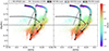 |
Fig. 3. Data compared to our models and to previous results from the literature. The colour-coding of the models and the data show the [Fe/H] content as explained by the colour bar. In this case, the data are binned so as to show the mean value of [Fe/H] in each bin. The three circles plotted on the models mark the ages 0.3 Gyr, 1 Gyr, and 5 Gyr. The horizontal and diagonal black lines separate three different plane regions as denoted by Fernandes et al. (2023); the unevolved populations lie in the upper left region, the MW high-α in situ population lies in the upper right region; and the MW low-α in situ population lies in the lower region. Left panel: [Mg/Mn] versus [Fe/H] for REF MW model (colour coded black-edge line) and NEW MW model (colour-coded white-edged line) compared to the APOGEE DR17 data of Fernandes et al. (2023) and their best model obtained adopting the prescriptions of Andrews et al. (2017; thin black line). Right panel: [Mg/Mn] versus [Fe/H] for REF MW model (colour-coded black-edge line) and MIX MW model (colour coded grey-edge line) compared to the same data and model by Fernandes et al. (2023). |
The plane is divided into three regions, according to what is usually done in the literature (see Fernandes et al. 2023 and references therein), by the horizontal and the diagonal black lines. This subdivision helps in identifying different populations of stars. The upper left sector has been interpreted as the locus of the unevolved stars, the upper right one as the location of the high-α in situ population, and the lower region as the low-α in situ population locus.
In both the panels we show the data, our REF MW model predictions (colour-coded black-edge line) and the results by Fernandes et al. (2023; black thin line). As the REF MW model did not reproduce the trends of Mg and Al, it does not even reproduce the trend shown by the data in this plane and, in particular, it shows a large underproduction of Al at low [Fe/H], which was also evident in the [Al/Fe] versus [Fe/H] plot. On the contrary, the obtained [Fe/H] range is in good agreement with the data, meaning that our choice of applying a small-effect correction on the Fe yield is quite reasonable.
In the left panel, we also show the NEW MW model with the yields corrected as in Table 2 (colour-coded white-edge model). It is evident that this second model better reproduces the data, matching the [Fe/H] range at the same time. The corrections that have the larger effect on this plane are those on Al and Fe, because their global effect is increasing the [Al/Fe] abundance. The corrections on Mg and Mn yields, on the other side, are less evident in this plane because they increase the production of both Mg and Mn; hence, the effect is smoothed out when we study the ratio between them.
In the right panel we show, together with the REF MW model, the MIX MW model. As presented in Table 3 this model is the combination of the prescription of the REF MW and the NEW MW models. It adopts the corrections for Mg and Al and the original prescriptions for Mn so that we are able to reproduce all the abundances. As is evident from the right panel, we can also fit the [Mg/Mn] versus [Al/Fe] trend; therefore, we can consider this combination of yields as the best one to reproduce the MW abundance features.
4.3. LMC: [Mg/Fe], [Al/Fe], and [Mn/Fe]
In this section we show the results we obtained with the LMC models regarding the abundances of Mg, Al, and Mn. For this dwarf galaxy we tested the REF LMC model (black line) and the NEW LMC model (white line), which contains the same yield corrections applied to the MW. Again, we do not show the MIX LMC model since it is just a combination of the other two. We show the abundance ratio predicted compared to the observed ones in Fig. 4. In this case, we see that although none of the two models is able to properly reproduce the abundance patterns observed, the NEW LMC models show a slight improvement. The case of Mn is noteworthy; the corrective factor that in the MW increases the Mn predicted by the model, when applied to the LMC decreases the Mn production substantially. This is easily understood by looking at the Mn corrective factor itself listed in Table 2. Since the factor is metallicity dependent, its effect on the abundance depends on the environment.
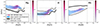 |
Fig. 4. LMC abundance ratios of Mg, Al, and Mn. The data are from APOGEE DR17 and are binned and colour-coded as in Fig. 2. Again, the blue line represents the running median computed with the same bin size and overlap, and the blue area is the standard deviation. The black and the white lines are the REF LMC model and the NEW LMC model, respectively. |
4.4. LMC: [Mg/Mn] versus [Al/Fe]
In this section, we show Fig. 5 with the results for the LMC in the plane [Mg/Mn] versus [Al/Fe] compared to the APOGEE DR17 data for LMC and the previous results presented by Fernandes et al. (2023). The models and the data follow the same colour-coding as in Fig. 3 as well as the division of the plane into three regions and the circles. In this case, the data are not binned since the data set is smaller than for the MW.
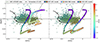 |
Fig. 5. LMC in [Mg/Mn] versus [Fe/H] plane. In the two panels, we plot our models compared to the APOGEE DR17 data and the model from Fernandes et al. (2023). As in Fig. 3 the colour-coding represents the [Fe/H] content. Again, the circles on the models mark three ages, 0.3 Gyr, 1 Gyr, and 5 Gyr. Here, unlike Fig. 3, the data are not binned. Left panel: REF LMC model (colour-coded black-edge line) and NEW LMC (with yields corrections, colour-coded white-edge line) are compared to data and to results of Fernandes et al. (2023). Right panel: REF LMC model (colour-coded black-edge line) and MIX LMC model (colour-coded grey-edge line) together with data and results of Fernandes et al. (2023). |
The interesting aspect of this plot is the location of the data and the model results on the plane. As already explained, the upper left part of the diagram is the locus of the unevolved populations, where around half of the LMC data points are located. The other half occupies the evolved region closer to the centre of the plot. In this context, the comparison between the LMC and the other nearby dwarf systems is noteworthy. As shown in Fernandes et al. (2023), the smallest satellites (e.g. Sculptor, Carina, Fornax, Draco, Sextans, and Ursa Minor), which are those with an SFR that was quenched at early times, tend to occupy the leftmost region of the plane, whereas the LMC is located more towards the centre of the diagram (with coordinates [Mg/Mn] ∼ 0.25 dex and [Al/Fe] ∼ −0.10 dex ). This difference could be a consequence of the SFH of the LMC, which presents active star formation at the present time, at variance with the other dwarf spheroidal galaxies. In our models, we adopted this kind of SFR and we were able to reproduce the observed evolution towards the centre of the plot. On the contrary, the MW has a present day star formation lower than the initial peak, and this produces an opposite evolution, from the right to the left of the plot.
As in Fig. 3, we show two panels displaying the models adopted. In both panels we show the data compared to the REF LMC model (colour-coded black-edge line) and to the results by Fernandes et al. (2023; thin black line) based on the LMC prescriptions by Andrews et al. (2017). It is evident that this model cannot reproduce the observations due to a too small Mg abundance and a too large Mn abundance. In the left panel, we compare these two trends with the NEW LMC model. This model does not reproduce the data either, but it represents an improvement with respect to the reference one. In particular, as shown in Fig. 5, the [Mg/Mn] predicted is substantially improved. In the right panel, we compare the REF LMC model to the MIX LMC model, which for the MW resulted to be the best one.
To highlight the best model among the three tested from a quantitative point of view, we computed the average [Mg/Mn] weighted on the stars formed in each time step and compared it to the average [Mg/Mn] obtained from the data. The REF MW model has an average [Mg/Mn] of ∼−0.32 dex, for the NEW LMC model the average [Mg/Mn] is ∼0.16 dex, and for the MIX LMC model it is ∼−0.29. The data on the other side show an average [Mg/Mn] of ∼0.23, which is in much better agreement with the result from the NEW LMC model.
The reason for the behaviour of the different models lies in the Mn yield. In the case of the MW, the original Mn prescription was the best one to reproduce the data, whereas for the LMC, even though none of the models overlap the running median, the new prescriptions work slightly better. Therefore, the NEW LMC model is the best one to describe the LMC.
4.5. Testing different nucleosynthesis and IMF prescriptions
Fernandes et al. (2023) compared APOGEE DR17 data with the predictions obtained by the chemical evolution models of Andrews et al. (2017). Therefore, in addition to our models, we also tested their nucleosynthesis prescriptions: they used the same sets of yields except for massive stars, where they adopted Chieffi & Limongi (2004). We tested this combination of yields for the MW in order to show how sensitive the [Mg/Mn] versus [Al/Fe] plane is to the nucleosynthesis prescriptions. We label this test model as the CL04 MW model, and we show the results compared to the data and to the REF MW model in Fig. 6. Here, we can see that by changing only the yields for the massive stars and no other parameters, we obtain a behaviour substantially different from the reference case shown in Fig. 3. Since we modified the production from massive stars, the differences concern the first part of the evolution of the Galaxy due to the massive star explosion timescales. Nevertheless, it is evident that we cannot reproduce the abundance pattern or the [Fe/H] range.
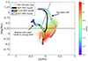 |
Fig. 6. [Mg/Mn] versus [Al/Fe] for CL04 MW model (colour-coded line, black edge) and K01 MW model (colour-coded line, white edge) compared to APOGEE DR17 data and REF MW model (black line). The colour-coding of the data, the CL04 MW model, and the K01 MW model is the same as Fig. 3, as are the binning of the data and the three circles plotted on the model. |
The reason for this is that the nucleosynthesis of the elements considered in this plot is quite uncertain. Mg is known to be underestimated by many different sets of yields, the nucleosynthesis of Mn is quite uncertain (Mn being a Fe-peak element), and that of Al has a dependence on the metallicity that introduces a further level of complexity. Hence, the adoption of the ratios of the above elements makes it quite difficult to draw firm conclusions. By changing the yields of these elements within their uncertainties one can obtain trends on the [Mg/Mn] versus [Al/Fe] plot with different behaviours, slopes, and [Fe/H] ranges.
In principle, the combination of these elements would allow us to disentangle some properties of the galaxies analysed, such as the SFR. However, given the state-of-the-art yields available in the literature, the nuclear uncertainties prevent this plane from being a strong diagnostic for the SFH of a galaxy.
We performed a second comparison with Fernandes et al. (2023) adopting all the parameters of REF MW model except the IMF, for which we adopted the one they used, namely Kroupa (2001). We show this model in Fig. 6. The Kroupa (2001) IMF is a top-heavy IMF that produces more massive stars than the Kroupa et al. (1993) that we adopted in the REF MW model and that was derived for the MW. The Kroupa (2001) IMF produces a more rapid increase of the metallicity than the Kroupa et al. (1993) one, and the net result is an increase of the [Al/Fe] ratios and the range in [Fe/H], relatively to the other models, as highlighted by the colour-coding in the figure.
The reason for choosing the Kroupa et al. (1993) IMF instead of the more recent Kroupa (2001) one is that the former was specifically derived for the solar vicinity, while the latter is a sort of universal IMF. Many previous papers on the MW have suggested the Kroupa et al. (1993) IMF as the best one to reproduce the main features of the Galactic disc (see e.g. Romano et al. 2010). For external galaxies, such as the satellites of the MW, the situation is different because no observational derivation of the IMF exists. In these cases, a Salpeter IMF is usually used, and this IMF is similar to the Kroupa (2001) one.
4.6. The effects of Galactic wind
Fernandes et al. (2023) compared APOGEE data with the predictions of the chemical evolution model proposed by Andrews et al. (2017), where a Galactic wind is assumed for the MW. In our REF MW and NEW MW models, we do not include any outflow since, for a potential well such as that of the MW, only Galactic fountains are allowed (Melioli et al. 2008, 2009; Spitoni et al. 2008, 2009). Therefore, for comparison with the Andrews et al. (2017) model, we computed a model for the MW with Galactic wind (WIND MW model; see Table 1). The introduction of the wind term into the chemical evolution equation works as a depletion term that decreases the gas available for the star formation. The net effect is that of a decline in the SFR (see Fig. 7), with fewer stars formed and therefore a lower abundance of metals restored into the interstellar medium. The wind affects the abundances in a very clear way, since the abundance ratios of elements produced on different timescales, for example [Mg/Mn] (in the case of a wind independent of the chemical species), drop drastically, because the effect of the gas loss is immediate on the elements produced on short timescales (e.g. Mg) and therefore related to the SFR. Mathematically, the intensity of the wind depends on the mass loading factor ωi, as shown in Sect. 2.2. In our case, we required it to be equal to 2.5, as was done by Andrews et al. (2017). Regarding the other prescriptions the WIND MW model follows the NEW MW model. In Fig. 8, we show that the WIND MW model, which is in the [Mg/Mn] versus [Al/Fe] plane, is shifted towards smaller values of both the abundance ratios. In addition, the range of [Fe/H] spanned by the WIND MW model is consistently lower than that spanned by the data, as shown by the colour-coding. In conclusion, once we add the wind to our models we are no longer able to properly reproduce the data trend or the range in [Fe/H].
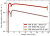 |
Fig. 7. SFHs for MW models without wind contribution (red line) and for WIND MW model (pink line) at 8 kpc from Galactic centre, compared to observed data (see reference in Fig. 1). |
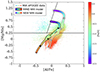 |
Fig. 8. [Mg/Mn] versus [Al/Fe] for WIND MW model (colour-coded line, black edge) and NEW MW model (colour-coded line, white edge) compared to APOGEE DR17 data. The colour-coding is the same as Fig. 3, as are the binning of the data and the circles plotted on the model. |
5. Conclusions
In this work, we studied the chemical evolution of the MW and of the LMC in order to understand the role of the [Mg/Mn] versus [Al/Fe] plane in unveiling the SFH of galaxies. According to the observational data, different stellar populations belonging to the same galaxy lie in different regions of the plane (as explained in Sect. 4.2). Hence, the galaxy pattern in this diagram is the result of the imprints left on those abundances by the SFH of that specific galaxy. In principle, this element combination is ideal for extracting information about the SFH, since they have different sites and timescales of production, but a discussion on the related uncertainties was still missing from the literature. Our aim was to analyse the uncertainties, in particular those related to the nucleosynthesis of these elements.
We did that by means of three already tested models for the MW and three for the LMC, where we varied the nucleosynthesis prescriptions. We also introduced a fourth model for the MW adopting the same yields from massive stars as in Andrews et al. (2017), with the aim of showing how the trends on the [Mg/Mn] versus [Al/Fe] plane depend on the assumed stellar nucleosynthesis.
Analysing the [Mg/Mn] versus [Al/Fe] for the different models presented, our results can be summarised as follows.
-
To reproduce the abundance patterns of Mg, Al, and Mn in the MW as shown by APOGEE DR17 data, it is necessary to add corrective factors to the yields adopted in Vasini et al. (2022). In particular, as shown in Table 2, we modified the massive stars’ contributions for Fe, Mg, and Al; the low-intermediate-mass star contribution for Al; and the SNIa production for Mn.
-
Regarding the LMC [Mg/Mn] versus [Al/Fe] diagram, the corrected yields also improve the agreement with the APOGEE data for this galaxy. This means that, even if the corrective factors were tailored to the MW, they also work for the LMC. At the same time, the recent SFR bursts, assumed for the LMC, account for those stars found on the evolved star region.
-
Changing the yields for massive stars only, as shown in Fig. 6, produces completely different results. By assuming different sets of yields one can obtain very different behaviours of the [Mg/Mn] versus [Al/Fe], as well as the predicted range of [Fe/H]. In the same way, also changing the IMF by adopting a top-heavy one modifies the behaviour on the [Mg/Mn] versus [Al/Fe] plane, predicting larger [Al/Fe] ratios, since the fraction of massive stars, which produce Al, is larger. In the work of Andrews et al. (2017), which computed the same diagram for the MW and satellite galaxies, the yields of CL04, the Kroupa (2001) IMF, and the presence of galactic winds in the MW are adopted. Their predicted trends marginally fit the data, and in some cases they are different from ours. In our standard model, we did not adopt the galactic winds in the MW, since it is more probable that in our Galaxy the gas produces Galactic fountains rather than winds, due to the deep potential well. However, we also computed a model including the Galactic wind with the same parameters as in Andrews et al. (2017), and the results produce a worse agreement with data than our standard model without wind.
-
Unfortunately, no firm conclusions are possible on the basis of theoretical models, mainly because of the uncertainties still present in the stellar yields and the IMF in our Galaxy and its satellites, the two quantities that most influence the abundance ratios.
In conclusion, this work focused on an issue that is not only related to the [Mg/Mn] versus [Al/Fe] plane, but also to all the other chemical elements. Many sets of stellar yields are available in the literature, but they differ from one another due to different nucleosynthesis and stellar evolution prescriptions and the presence or absence of mass loss and rotation. In addition, there are some elements whose nucleosynthesis is very poorly known, and among those elements are, indeed, Mn and Al. Therefore, it is risky to rely only on one diagram, such as that discussed in this paper. Other chemical clocks should be adopted at the same time, such as s-process elements and alpha elements relative to Fe, coupled with the kinematic properties.
Acknowledgments
The authors kindly thank the referee for all the interesting comments and suggestions that improved substantially the paper. We also thank INAF for the 1.05.12.06.05 Theory Grant – Galactic archaeology with radioactive and stable nuclei.
References
- Abdurro’uf, Accetta, K., Aerts, C., et al. 2022, ApJS, 259, 35 [NASA ADS] [CrossRef] [Google Scholar]
- Ahumada, R., Allende Prieto, C., Almeida, A., et al. 2020, ApJS, 249, 3 [NASA ADS] [CrossRef] [Google Scholar]
- Andrews, B. H., Weinberg, D. H., Schönrich, R., & Johnson, J. A. 2017, ApJ, 835, 224 [NASA ADS] [CrossRef] [Google Scholar]
- Carrillo, A., Deason, A. J., Fattahi, A., Callingham, T. M., & Grand, R. J. J. 2024, MNRAS, 527, 2165 [Google Scholar]
- Cescutti, G., Matteucci, F., Lanfranchi, G. A., & McWilliam, A. 2008, A&A, 491, 401 [NASA ADS] [CrossRef] [EDP Sciences] [Google Scholar]
- Chiappini, C., Matteucci, F., & Gratton, R. 1997, ApJ, 477, 765 [Google Scholar]
- Chiappini, C., Matteucci, F., & Romano, D. 2001, ApJ, 554, 1044 [NASA ADS] [CrossRef] [Google Scholar]
- Chieffi, A., & Limongi, M. 2004, ApJ, 608, 405 [NASA ADS] [CrossRef] [Google Scholar]
- Das, P., Hawkins, K., & Jofré, P. 2020, MNRAS, 493, 5195 [NASA ADS] [CrossRef] [Google Scholar]
- Feltzing, S., & Feuillet, D. 2023, ApJ, 953, 143 [NASA ADS] [CrossRef] [Google Scholar]
- Fernandes, L., Mason, A. C., Horta, D., et al. 2023, MNRAS, 519, 3611 [NASA ADS] [CrossRef] [Google Scholar]
- Feuillet, D. K., Sahlholdt, C. L., Feltzing, S., & Casagrande, L. 2021, MNRAS, 508, 1489 [NASA ADS] [CrossRef] [Google Scholar]
- François, P., Matteucci, F., Cayrel, R., et al. 2004, A&A, 421, 613 [NASA ADS] [CrossRef] [EDP Sciences] [Google Scholar]
- Gaia Collaboration (Recio-Blanco, A., et al.) 2023, A&A, 674, A38 [CrossRef] [EDP Sciences] [Google Scholar]
- Grisoni, V., Spitoni, E., & Matteucci, F. 2018, MNRAS, 481, 2570 [NASA ADS] [Google Scholar]
- Harris, J., & Zaritsky, D. 2009, AJ, 138, 1243 [NASA ADS] [CrossRef] [Google Scholar]
- Hawkins, K., Jofré, P., Masseron, T., & Gilmore, G. 2015, MNRAS, 453, 758 [NASA ADS] [CrossRef] [Google Scholar]
- Helmi, A., Babusiaux, C., Koppelman, H. H., et al. 2018, Nature, 563, 85 [Google Scholar]
- Holtzman, J. A., Shetrone, M., Johnson, J. A., et al. 2015, AJ, 150, 148 [Google Scholar]
- Horta, D., Schiavon, R. P., Mackereth, J. T., et al. 2023, MNRAS, 520, 5671 [NASA ADS] [CrossRef] [Google Scholar]
- Iwamoto, K., Brachwitz, F., Nomoto, K., et al. 1999, ApJS, 125, 439 [NASA ADS] [CrossRef] [Google Scholar]
- José, J., & Hernanz, M. 1998, ApJ, 494, 680 [Google Scholar]
- Karakas, A. I. 2010, MNRAS, 403, 1413 [NASA ADS] [CrossRef] [Google Scholar]
- Kennicutt, R. C., Jr. 1998, ApJ, 498, 541 [Google Scholar]
- Kobayashi, C., Umeda, H., Nomoto, K., Tominaga, N., & Ohkubo, T. 2006, ApJ, 653, 1145 [NASA ADS] [CrossRef] [Google Scholar]
- Kroupa, P. 2001, MNRAS, 322, 231 [NASA ADS] [CrossRef] [Google Scholar]
- Kroupa, P., Tout, C. A., & Gilmore, G. 1993, MNRAS, 262, 545 [NASA ADS] [CrossRef] [Google Scholar]
- Lian, J., Thomas, D., Maraston, C., et al. 2020, MNRAS, 497, 2371 [Google Scholar]
- Majewski, S. R., Schiavon, R. P., Frinchaboy, P. M., et al. 2017, AJ, 154, 94 [NASA ADS] [CrossRef] [Google Scholar]
- Matteucci, F., & Francois, P. 1989, MNRAS, 239, 885 [Google Scholar]
- Melioli, C., Brighenti, F., D’Ercole, A., & de Gouveia Dal Pino, E. M. 2008, MNRAS, 388, 573 [Google Scholar]
- Melioli, C., Brighenti, F., D’Ercole, A., & de Gouveia Dal Pino, E. M. 2009, MNRAS, 399, 1089 [Google Scholar]
- Montalbán, J., Mackereth, J. T., Miglio, A., et al. 2021, Nat. Astron., 5, 640 [Google Scholar]
- Myeong, G. C., Vasiliev, E., Iorio, G., Evans, N. W., & Belokurov, V. 2019, MNRAS, 488, 1235 [Google Scholar]
- Nidever, D. L., Hasselquist, S., Hayes, C. R., et al. 2020, ApJ, 895, 88 [Google Scholar]
- Perottoni, H. D., Limberg, G., Amarante, J. A. S., et al. 2022, ApJ, 936, L2 [NASA ADS] [CrossRef] [Google Scholar]
- Prantzos, N., Abia, C., Limongi, M., Chieffi, A., & Cristallo, S. 2018, MNRAS, 476, 3432 [Google Scholar]
- Romano, D., & Matteucci, F. 2003, MNRAS, 342, 185 [Google Scholar]
- Romano, D., Karakas, A. I., Tosi, M., & Matteucci, F. 2010, A&A, 522, A32 [NASA ADS] [CrossRef] [EDP Sciences] [Google Scholar]
- Salpeter, E. E. 1955, ApJ, 121, 161 [Google Scholar]
- Spitoni, E., Recchi, S., & Matteucci, F. 2008, A&A, 484, 743 [NASA ADS] [CrossRef] [EDP Sciences] [Google Scholar]
- Spitoni, E., Matteucci, F., Recchi, S., Cescutti, G., & Pipino, A. 2009, A&A, 504, 87 [NASA ADS] [CrossRef] [EDP Sciences] [Google Scholar]
- Spitoni, E., Vincenzo, F., Matteucci, F., & Romano, D. 2016, MNRAS, 458, 2541 [Google Scholar]
- Spitoni, E., Silva Aguirre, V., Matteucci, F., Calura, F., & Grisoni, V. 2019, A&A, 623, A60 [NASA ADS] [CrossRef] [EDP Sciences] [Google Scholar]
- Tolstoy, E., Hill, V., & Tosi, M. 2009, ARA&A, 47, 371 [Google Scholar]
- Vasini, A., Matteucci, F., & Spitoni, E. 2022, MNRAS, 517, 4256 [NASA ADS] [CrossRef] [Google Scholar]
- Vasini, A., Matteucci, F., Spitoni, E., & Siegert, T. 2023, MNRAS, 523, 1153 [NASA ADS] [CrossRef] [Google Scholar]
All Tables
Parameters of the five MW and two LMC models tested (indicated in the first column).
All Figures
|
Fig. 1. SFHs predicted by Vasini et al. (2022, 2023) and used in the paper. For the MW (red line), the Kennicutt (1998) law with exponent k = 1.5 was adopted, and the temporal evolution of the star formation at the solar ring (8 kpc) is compared with the present-day observed SFR (vertical yellow line, data taken from Prantzos et al. 2018). For the LMC (blue line) we assumed a linear Kennicutt (1998) law with a variable efficiency to reproduce the Harris & Zaritsky (2009) SFR. We compared it with the observation at the present time by Harris & Zaritsky (2009) itself (vertical cyan line). |
| In the text | |
|
Fig. 2. Abundance ratios of the three elements involved. The data are from APOGEE DR17 and are binned and colour-coded according to the data density in each bin. The blue line represents the running median, computed assuming a bin size of 0.1 dex and an overlap of 0.025 dex, and the blue shaded area represents the related standard deviation. Left panel: [Mg/Fe] in the MW as predicted by REF MW model (black line) and by NEW MW model (white line) compared to APOGEE data. Middle panel: [Al/Fe] MW abundance for both models (same colour-coding as left panel). Right panel: [Mn/Fe] abundance for REF MW and NEW MW models (same colour-coding). |
| In the text | |
|
Fig. 3. Data compared to our models and to previous results from the literature. The colour-coding of the models and the data show the [Fe/H] content as explained by the colour bar. In this case, the data are binned so as to show the mean value of [Fe/H] in each bin. The three circles plotted on the models mark the ages 0.3 Gyr, 1 Gyr, and 5 Gyr. The horizontal and diagonal black lines separate three different plane regions as denoted by Fernandes et al. (2023); the unevolved populations lie in the upper left region, the MW high-α in situ population lies in the upper right region; and the MW low-α in situ population lies in the lower region. Left panel: [Mg/Mn] versus [Fe/H] for REF MW model (colour coded black-edge line) and NEW MW model (colour-coded white-edged line) compared to the APOGEE DR17 data of Fernandes et al. (2023) and their best model obtained adopting the prescriptions of Andrews et al. (2017; thin black line). Right panel: [Mg/Mn] versus [Fe/H] for REF MW model (colour-coded black-edge line) and MIX MW model (colour coded grey-edge line) compared to the same data and model by Fernandes et al. (2023). |
| In the text | |
|
Fig. 4. LMC abundance ratios of Mg, Al, and Mn. The data are from APOGEE DR17 and are binned and colour-coded as in Fig. 2. Again, the blue line represents the running median computed with the same bin size and overlap, and the blue area is the standard deviation. The black and the white lines are the REF LMC model and the NEW LMC model, respectively. |
| In the text | |
|
Fig. 5. LMC in [Mg/Mn] versus [Fe/H] plane. In the two panels, we plot our models compared to the APOGEE DR17 data and the model from Fernandes et al. (2023). As in Fig. 3 the colour-coding represents the [Fe/H] content. Again, the circles on the models mark three ages, 0.3 Gyr, 1 Gyr, and 5 Gyr. Here, unlike Fig. 3, the data are not binned. Left panel: REF LMC model (colour-coded black-edge line) and NEW LMC (with yields corrections, colour-coded white-edge line) are compared to data and to results of Fernandes et al. (2023). Right panel: REF LMC model (colour-coded black-edge line) and MIX LMC model (colour-coded grey-edge line) together with data and results of Fernandes et al. (2023). |
| In the text | |
|
Fig. 6. [Mg/Mn] versus [Al/Fe] for CL04 MW model (colour-coded line, black edge) and K01 MW model (colour-coded line, white edge) compared to APOGEE DR17 data and REF MW model (black line). The colour-coding of the data, the CL04 MW model, and the K01 MW model is the same as Fig. 3, as are the binning of the data and the three circles plotted on the model. |
| In the text | |
|
Fig. 7. SFHs for MW models without wind contribution (red line) and for WIND MW model (pink line) at 8 kpc from Galactic centre, compared to observed data (see reference in Fig. 1). |
| In the text | |
|
Fig. 8. [Mg/Mn] versus [Al/Fe] for WIND MW model (colour-coded line, black edge) and NEW MW model (colour-coded line, white edge) compared to APOGEE DR17 data. The colour-coding is the same as Fig. 3, as are the binning of the data and the circles plotted on the model. |
| In the text | |
Current usage metrics show cumulative count of Article Views (full-text article views including HTML views, PDF and ePub downloads, according to the available data) and Abstracts Views on Vision4Press platform.
Data correspond to usage on the plateform after 2015. The current usage metrics is available 48-96 hours after online publication and is updated daily on week days.
Initial download of the metrics may take a while.