| Issue |
A&A
Volume 682, February 2024
|
|
|---|---|---|
| Article Number | L24 | |
| Number of page(s) | 8 | |
| Section | Letters to the Editor | |
| DOI | https://doi.org/10.1051/0004-6361/202348756 | |
| Published online | 27 February 2024 | |
Letter to the Editor
Constraints on the evolution of the Triton atmosphere from occultations: 1989–2022
1
LESIA, Observatoire de Paris, Université PSL, CNRS, Sorbonne Université, 5 place Jules Janssen, 92190 Meudon, France
e-mail: Bruno.Sicardy@obspm.fr
2
Indian Institute of Space Science and Technology, Thiruvananthapuram, 695547 Kerala, India
3
Federal University of Uberlândia (UFU), Physics Institute, Av. João Naves de Ávila 2121, Uberlândia, MG 38408-100, Brazil
4
Laboratório Interinstitucional de e-Astronomia – LIneA, Av. Pastor Martin Luther King Jr 126, Rio de Janeiro, RJ 20765-000, Brazil
5
American Association of Variable Star Observers (AAVSO), 185 Alewife Brook Parkway, Suite 410, Cambridge, MA 02138, USA
6
Physical Research Laboratory, Ahmedabad, 380009 Gujarat, India
7
Universidade do Rio de Janeiro – Observatório do Valongo, Ladeira do Pedro Antonio 43, Rio de Janeiro, RJ 20.080-090, Brazil
8
Institut Polytechnique des Sciences Avancées IPSA, 94200 Ivry-sur-Seine, France
9
IMCCE, Observatoire de Paris, PSL Research University, CNRS, Sorbonne Université, Univ. Lille, 75014 Paris, France
10
Observatório Nacional/MCTIC, Rio de Janeiro, Brazil
11
TÜBITAK National Observatory, Akdeniz University Campus, Antalya 07058, Turkey
12
Instituto de Astrofísica de Andalucía (IAA-CSIC), Glorieta de la Astronomía s/n, 18008 Granada, Spain
13
Federal University of Technology-Paraná (UTFPR/PPGFA), Curitiba, PR, Brazil
14
Tata Institute of Fundamental Research, Homi Bhabha Road, Colaba, Mumbai 400 005, India
15
Indian Institute of Astrophysics, II Block, Koramangala, Bangalore 560034, India
16
Department of Physics, Indian Institute of Technology Bombay, Powai 400 076, India
17
Aryabhatta Research Institute of Observational Sciences, Manora Peak, Nainital 263002, India
18
Akashmitra Mandal, Kalyan, 421301 Maharashtra, India
19
Nicolaus Copernicus Astronomical Center, Polish Academy of Sciences, ul. Rabiańska 8, 87-100 Toruń, Poland
20
Udaipur Solar Observatory, Physical Research Laboratory, PO Box 198 Badi Road, 313001 Udaipur, India
21
Harvard College Observatory, Harvard University, 60 Garden St., Cambridge, 02158 MA, USA
22
Department of Astronomy, Stockholm University, AlbaNova University Center, 10691 Stockholm, Sweden
23
INAF, Osservatorio Astrofisico di Catania, Via S. Sofia 78, 95123 Catania, Italy
24
Key Laboratory for Research in Galaxies and Cosmology, Chinese Academy of Sciences, 80 Nandan Rd., Shanghai 200030, PR China
25
School of Astronomy and Space Science, University of Chinese Academy of Sciences, 1 East Yanqi Lake Rd., Beijing 100049, PR China
26
Key Lab of Space Astronomy and Technology, National Astronomical Observatories, Beijing, 100101 PR China
27
Shandong Astronomical Society, 180 West Wenhua Rd., Weihai, Shandong 264209, PR China
28
Vygonnaia street, house 2/1, flat 59, Ussuriysk, Primorsky Krai 692527, Russia
29
Koshkina Street, house 19 k. 1, flat 210, Moscow 115409, Russia
30
SETI Institute, 339 N Bernardo Ave Suite 200, Mountain View, CA 94043, USA
31
Unistellar, 5 allée Marcel Leclerc, bâtiment B, Marseille 13008, France
32
Unistellar Citizen Scientist, Tsuchiura, Japan
33
Unistellar Citizen Scientist, Kagoshima, Japan
34
UNESP-São Paulo State University, Grupo de Dinâmica Orbital e Planetologia, CEP 12516-410 Guaratinguetá, SP, Brazil
Received:
28
November
2023
Accepted:
2
February
2024
Context. In about 2000, the south pole of Triton experienced an extreme summer solstice that occurs every ∼650 years, when the subsolar latitude reached about 50°S. Bracketing this epoch, a few occultations probed the Triton atmosphere in 1989, 1995, 1997, 2008, and 2017. A recent ground-based stellar occultation observed on 6 October 2022 provides a new measurement of the atmospheric pressure on Triton. This is presented here.
Aims. The goal is to constrain the volatile transport models (VTMs) of the Triton atmosphere. The atmosphere is basically in vapor pressure equilibrium with the nitrogen ice at its surface.
Methods. Fits to the occultation light curves yield the atmospheric pressure of Triton at the reference radius 1400 km, from which the surface pressure is deduced.
Results. The fits provide a pressure p1400 = 1.211 ± 0.039 μbar at radius 1400 km (47 km altitude), from which a surface pressure of psurf = 14.54 ± 0.47 μbar is deduced (1σ error bars). To within the error bars, this is identical to the pressure derived from the previous occultation of 5 October 2017, p1400 = 1.18 ± 0.03 μbar and psurf = 14.1 ± 0.4 μbar, respectively. Based on recent models of the volatile cycles of Triton, the overall evolution of the surface pressure over the last 30 years is consistent with N2 condensation taking place in the northern hemisphere. However, models typically predict a steady decrease in the surface pressure for the period 2005-2060, which is not confirmed by this observation. Complex surface-atmosphere interactions, such as ice albedo runaway and formation of local N2 frosts in the equatorial regions of Triton, could explain the relatively constant pressure between 2017 and 2022.
Key words: planets and satellites: atmospheres / planets and satellites: individual: Triton
© The Authors 2024
 Open Access article, published by EDP Sciences, under the terms of the Creative Commons Attribution License (https://creativecommons.org/licenses/by/4.0), which permits unrestricted use, distribution, and reproduction in any medium, provided the original work is properly cited.
This article is published in open access under the Subscribe to Open model. Subscribe to A&A to support open access publication.
1. Introduction
Triton is the largest of the Neptune satellites. Together with the Saturnian satellite Titan, it is the only satellite known to possess a global atmosphere. The Triton atmosphere was revealed during the NASA Voyager 2 (V2) flyby of the main Neptunian satellite in August 1989. The Radio Science Subsystem (RSS; Tyler et al. 1989; Gurrola 1995) occultation provided a surface pressure of psurf = 14 ± 1 μbar (1σ level). Combined with other V2 data and subsequent ground-based observations, it was seen that the tenuous atmosphere of Triton is mainly composed of nitrogen, N2, in vapor pressure equilibrium with the icy surface.
Since 1989, a handful of Earth-based observations of stellar occultations monitored the Triton atmosphere. The events on 15 August 1995 (Olkin et al. 1997), 18 July 1997 (Elliot et al. 2000 and Marques Oliveira et al. 2022; MO22 hereafter), and 4 November 1997 (Elliot et al. 2003) indicated a significant increase in the pressure relative to the RSS measurement. No further constraints on the atmospheric pressure of Triton could be achieved from the 21 May 2008 occultation, which had a grazing geometry (MO22).
The 5 October 2017 ground-based occultation campaign provided the first dense coverage of the Triton atmosphere, with 90 occultation chords scanning both hemispheres of the satellite (MO22). Combined with the good signal-to-noise ratio of some of the light curves, this event yielded strong constraints on the thermal, density, and pressure profiles of this atmosphere between altitude levels of ∼8 km and ∼190 km (from ∼9 μbar and a few nanobars, respectively). In particular, the atmospheric pressure was found to have returned to the RSS value of 1989. Moreover, the detection and structure of a central flash revealed an essentially spherical atmosphere with an apparent oblateness lower than 0.0011 at the 8 km altitude level.
Triton has recently experienced a rare extreme southern solstice, which occurs every ∼650 years (see the details in Bertrand et al. 2022). The subsolar latitude on the satellite reached about 50°S in 2000. Seasonal variations in the surface pressure can then constrain volatile transport models (VTMs) that account for volatile transport induced by insolation changes. These models assume that the Triton atmosphere has a negligible radiative thermal influence on the energy balance of its surface. They calculate the local insolation at the surface and the thermal infrared cooling, the heat storage in regions covered by N2 ice and conduction in the subsurface, and, in the presence of N2 ice, the condensation-sublimation rates necessary to force the surface temperature to remain at the nitrogen frost point, which in turn depends on surface pressure. These processes are sufficient to estimate the temporal evolution of the surface temperature, pressure and N2 transport to first order.
The first numerical Triton VTMs emerged in the late 1980s, motivated by the V2 Triton flyby (Spencer 1990, Hansen & Paige 1992, Spencer & Moore 1992, Brown & Kirk 1994). The Triton atmosphere has similarities with that of Pluto (an N2 atmosphere controlled by vapor pressure equilibrium with the surface ices). Hence, crucial insights were gained after the Pluto New Horizons flyby in 2015, which allowed the VTMs for Triton to be updated in light of new observable constraints (MO22; Bertrand et al. 2022).
After the pressure increase noted in 1995 and 1997, the surface pressure in 2017 was found to be close to the V2 value (MO22). To first order, the volatile transport models have been able to reproduce this trend for a wide range of model parameters. The reason is that nitrogen ice sublimation peaked in the southern hemisphere in ∼2000–2005 as the southern N2 ice cap was under maximum insolation (summer solstice). However, the models of Bertrand et al. (2022) do not suggest a strong surge in surface pressure (see their Figs. 9, 10, and 21), as claimed from stellar occultations for the period 1995–1997 (e.g., Elliot et al. 2000), but instead predict a moderate increase, with a peak around 15–19 μbar for the surface pressure. However, other processes not taken into account in these models (e.g., ice albedo feedback) may have increased the peak amplitude during this period.
Here, we present results obtained from a new stellar occultation event observed on 6 October 2022 from ground-based (China and India) and space (CHEOPS1) facilities. These new results help constrain the evolution of the Triton atmosphere over the period 1989–2022. This is a timely event, considering how rare Triton occultations are, owing to the depleted stellar fields that are currently crossed by the Neptune system as seen from Earth.
2. Observations
The Triton occultation campaign of 6 October 2022 was organized under the auspices of the Lucky Star project2. Comprehensive details regarding the event can be found in a dedicated web page3. The compilation and management of the observational data are facilitated by Lucky Star’s Occultation Portal website4 (Kilic et al. 2022). The Gaia DR3 position at the epoch of occultation and the Triton ephemeris from previous occultation events were used for the final prediction (see Fig. 1).
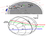 |
Fig. 1. Geometry of the 6 October 2022 stellar occultation by Triton. Upper panel: Dark blue lines (continued in red outside the Earth) delimit the predicted path of the Triton shadow on Earth on 6 October 2022. The shadow moves from right to left. The shadow centers (black dots) are spaced by one minute, and the larger black dot marks the geocentric closest approach near 14:39:46 UT (Table 1). Colors indicate stations at which the occultation was successfully detected. The blue arc shows the motion of the CHEOPS spacecraft during the event, while the red and green dots show Mt. Saraswati and Yanqi Lake, respectively. The white dots show the stations that were clouded out (see Table A.1). Lower panel: Reconstructed geometry of the occultation as seen in the sky plane. The J2000 celestial north (N) and east (E) directions and the scale are displayed in the upper right corner. The gray arrow near the equator shows the direction of rotation of the satellite. The (Neptune-facing) prime meridian is drawn as a thicker line than the other meridians, and the label S marks the south pole. The dotted circle indicates the layer in the Triton atmosphere that causes the half-light level (∼90 km altitude). The colored lines are the trajectories of the star relative to Triton (also known as occultation chords) as observed from various stations (see labels), and the black arrow indicates the direction of motion. The open circle is the predicted center of Triton, and the cross marks the actual center derived from the atmospheric fit. The offset between the two mainly stems from a correction of the Triton ephemeris. |
The occultation was successfully observed from space by CHEOPS. Two successful observations were obtained in India at Mt. Saraswati in the Himalayan region, and one light curve was successfully recorded at Yanqi Lake, China. Attempts from Devasthal, Uttarakhand (India), Mt. Abu and Dhanari, Rajasthan (India), Udaipur (India), Nakhodka (Russia) and three sites in Japan were clouded out (see details in Appendix A and Table A.1).
3. Data analysis
Our analysis used tools developed in the Platform for Reduction of Astronomical Images Automatically (PRAIA; Assafin 2023a,b)5 and the packages of the Stellar Occultation Reduction and Analysis (SORA; Gomes-Júnior et al. 2022)6.
The resulting occultation light curves were fit using the ray-tracing code that was initially developed for the Pluto atmosphere by Dias-Oliveira et al. (2015; see also Meza et al. 2019 and Sicardy et al. 2021). This code was adapted to the Triton atmosphere, using the parameters of MO22 (their Table 2) and those in Table 1 of this paper. The Triton atmosphere was assumed to be transparent and composed of pure N2, and we note that the CH4 abundance of 10−4 is negligible for our purposes. Further, we assumed it to be spherical, as supported by the shape of the central flash observed during the 5 October 2017 event (MO22).
Parameters of the occulted star and Triton, and results of the atmospheric fits.
The atmospheric thermal profile T(r) of Triton, where r is the distance to the Triton center, is the same as was used by MO22 (see their Figs. 10, 11 and B.1 and their Table B.1). It starts from the surface with a strong positive thermal gradient of 5 K km−1. This gradient decreases rapidly, and the temperature reaches a local maximum value of about 50 K at r = 1363 km (10 km altitude). This is followed by a mesosphere with a mild negative gradient of about −0.2 K km−1 centered around r = 1375 km (23 km altitude). This mesosphere finally connects with a thermosphere with a positive gradient of about 0.1 K km−1 above the 50 km altitude level.
A χ2 minimization procedure was applied by simultaneously fitting all the four light curves. The M = 7 free parameters of the fit were the pressure p1400 at the reference radius r = 1400 km, the offset (fc, gc) to apply to the Triton ephemeris along the celestial east and north directions, respectively, and the contributions of the Triton flux to the total Triton plus stellar flux in the four observed light curves. These contributions are different from one station to the next because the instruments used different filters (Table A.1), which induced variations in the magnitudes of both Triton and the star. The offset (fc, gc) was obtained by determining the shift in time Δt to apply to all the light curves and the cross-track offset to the Triton ephemeris, Δρ, that minimizes χ2.
The fit used a total N = 2398 data points, providing a χ2 value per degree of freedom  , where
  is the minimum value of χ2 obtained in the fitting procedure. The best fit to the data (Fig. 2) has a value
  , indicating a satisfactory modeling of the data. Figure 3 shows the map of χ2 versus the pressure p1400 at a radius of 1400 km and the cross-track offset Δρ. As summarized in Table 1, the fit provides a best-fit pressure of p1400 = 1.211 ± 0.039 μbar (1σ level). Our adopted temperature profile implies that psurf/p1400 = 12.01, yielding psurf = 14.54 ± 0.47 μbar.
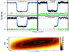 |
Fig. 2. Simultaneous fits of the data by synthetic light curves. Upper panel: Best fit to the data, shown as blue lines, using a Triton surface pressure of psurf = 14.54 μbar and other parameters provided in Table 1. The residuals (observations minus model) are shown in green. The lower and upper dotted horizontal lines mark the zero flux and the average flux of Triton plus the star, respectively. Each light curve is normalized to the total flux of Triton plus the star and is plotted over a time interval of 6 minutes. The red tick marks indicate 14:41:40 UT. The HCT light curve was binned over five data points (1.05-second time resolution) for a better comparison with the other light curves. We note that a faint central flash is present in the Yanqi Lake light curve. The 1σ error bars are obtained with the PRAIA software, which accounts for the instrumental and photon noises, knowing that the error bars for the CHEOPS data points are dominated by photon noise (see Appendix A). They are not visible here because they are smaller than the plotted dots. Lower panel: χ2 map of the simultaneous fits. The 1σ and 3σ level curves are shown in green. |
4. Pressure evolution
Figure 3 shows the measured values of the atmospheric pressure of Triton over the period 1989–2022, together with various VTM outputs of Bertrand et al. (2022). We considered the simulations of these authors performed with unlimited and fixed N2 ice reservoirs (i.e., no short-term frosts are involved) in the southern and northern hemispheres (see their Figs. 9–10), with some cases shown as dotted, dash-dotted, and dashed lines in Fig. 3.
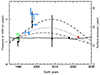 |
Fig. 3. Comparison of observations with VMT models. The figure shows the atmospheric pressure of Triton obtained from occultation measurements taken between 1989 and 2022 (see dates and values in Table 1). The red point is the result of the 6 October 2022 occultation (this work). It has been obtained using the same method as adopted by MO22 (black points). The green point (G95) is from the V2 RSS occultation of 25 August 1989 (Gurrola 1995). The blue points are O97, ground-based stellar occultation, 14 August 1995 (Olkin et al. 1997); E03, ground-based stellar occultation, 18 July 1997 (Elliot et al. 2000); E00, HST-based stellar occultation, 4 November 1997 (Elliot et al. 2003). It should be noted that MO22 analyzed the RSS data of August 1989 and the occultation data of July 1997 independently of Gurrola (1995) and Elliot et al. (2000), respectively. The vertical axes show the pressures at the reference radius 1400 km (left) and at the surface (right), assuming psurf/p1400 = 12.01 (see text). The lines are examples of VTM simulations by Bertrand et al. (2022). The dash-dotted line shows a model with the southern cap within 90°S–30°S and the northern cap within 45°N–90°N. The dotted line shows a case with the southern cap within 90°S–30°S and the northern cap within 60°N–90°. The dashed line shows another case with the southern cap within 90°S–30°S and no northern cap (volatile-free northern hemisphere). The solid line presents a simulation in which the N2 ice evolved freely over millions of years so that permanent and seasonal polar caps as well as local frost deposits can form self-consistently. In this simulation, the formation of thin seasonal N2 frosts is predicted in the current southern summer in the equatorial regions. None of the simulations fits the data satisfactorily. The dashed line accounts for the pressure increase of 1995–1997, but overestimates the pressures measured in 2017 and 2022. The dotted line marginally explains the increase of 1995–1997 and satisfactorily fits the 2022 measurement, but fails to explain the 2017 point. The dash-dotted line does not fit the increase of 1995–1997, while going through the 2017 point, but fails to explain the 2022 point. The solid line accounts for a basically constant pressure between 1989, 2017, and 2022, as well as the slight increases between 2017 and 2022. However, it is only marginally consistent with the 1995 result, and it does not account for the pressure surge of 1997. |
These simulations inevitably predict a steady decrease in pressure between 2005 and 2022, with a pressure in 2022 that is at least 5% lower than that in 2017 (and 5% in the case of the dash-dotted line in Fig. 3), followed by a steady decrease that is predicted to last for many decades. The reason is that as the subsolar point moves from the southern latitudes toward the equator in 2022, nitrogen sublimation becomes less intense over the southern reservoir of N2 ice, while condensation in the northern hemisphere and in the equatorial regions dominates sublimation on the global scale. This trend is also obtained in their simulations performed with limited N2 ice reservoirs and with seasonal frosts, which best match the observational constraints (see their Fig. 21), including the surface pressure in 1989 and 2017 and the latitudinal extent of the ice as suggested from V2 images, among others.
None of the simulations mentioned above can explain both the pressure surge observed in the 1990s and the return to the pressure of 1989 in 2017 and 2022 (Fig. 3).
Some simulations of Bertrand et al. (2022) obtain a relatively constant surface pressure between 1989, 2017, and 2022 that is consistent with our present result (Fig. 3, solid line). In these simulations, the N2 condensation is more intense in the northern hemisphere during this period because the seasonal northern cap is strongly extended equatorward in the form of frosts that cover tens of centimeters, due to a cold bedrock (typically, the bedrock surface bolometric albedo in these simulations is ≥0.9). This balances the sublimation in the southern hemisphere and causes the pressure to remain relatively constant between 1989 and 2022. However, these simulations (1) include extended N2 ice frosts to low northern latitudes in 1989, which seems inconsistent with the V2 images, unless the blue fringe observed in the equatorial regions correspond to a centimeter-thick N2 frost (see the discussions about the blue fringe in Bertrand et al. 2022, their Sect. 8.4), and in fact (2) they do not include a peak in pressure at all during the 1995–1997 period.
Nevertheless, this surge should be considered with caution. The black points in Fig. 3, taken from MO22, were all obtained using the same temperature profile T(r) and the same ray-tracing code. In contrast, the blue points were obtained with different methods that are also different from our approach. For instance, using the same data set from the 18 July 1997 occultation, Elliot et al. (2000) and MO22 derived p1400 = 2.23 ± 0.28 μbar and  μbar, respectively. Although these two values agree to within their respective error bars, they show that a consistent comparison between results obtained by various teams remains problematic. In this context, when we consider only the values p1400 = 1.0 ± 0.2 μbar and
  μbar derived by MO22 for the 25 August 1989 and 18 July 1997 measurements, respectively, then the surge in pressure between 1989 and 1997 reaches a moderate 2.5σ level.
However, the formation of local N2 frosts in the equatorial region during the period 1980–2020, which is very sensitive to surface properties or albedo feedback, may not be simulated in the VTM with sufficient details and could alter the pressure cycle. Another possibility is a significant role on Triton of albedos and ice composition feedback as geysers or haze particles could deposit dark material (or bright ice grain) on top of the ice, and further darken (brighten) the ice, and thus impact the N2 sublimation-condensation rates. These processes are not taken into account in the VTM, but were shown to be efficient runaway forcing mechanisms on Pluto (Earle et al. 2018; Bertrand et al. 2020). They might cause significant subseasonal atmospheric pressure variations in the Pluto atmosphere on timescales ranging from a few to tens of Earth years, as suggested by stellar occultations (see Arimatsu et al. 2020 and Yuan et al. 2023). Yuan et al. (2023) actually noted that short-term changes in the Pluto surface ices have been reported by Grundy et al. (2014), Lellouch et al. (2022) and Holler et al. (2022). This could reconcile the observations presented here in particular with the 1995-1997 surge of pressure of the Triton atmosphere. However, all the points evoked above remain speculative and should be explored in detail with the models.
5. Conclusions
The main constraint obtained here is that the atmospheric pressure of Triton is essentially the same in 1989, 2017, and 2022, regardless of what occurred in between. More specifically, the pressure changed very little between 2017 and 2022, with an insignificant increase of 0.031 ± 0.049 μbar (resp. 0.38 ± 0.59 μbar) between the two dates at 1400 km (or the surface).
It remains difficult to clearly assess the seasonal trend of the N2 cycle on Triton because the simulations from Bertrand et al. (2022) do not explain consistently all the available observations, that is, all pressure measurements over the 1989–2022 period and the visual appearance of the Triton surface in images of Voyager 2. Another issue is that our 2022 measurement is closer in time to the 2017 measurement compared to the seasonal timescale on Triton (∼40 years). Complex processes that are not taken into account in the VTMs could occur and perturb the N2 cycle over a short timescale of 5 years, thus temporarily masking the seasonal trend (see the discussion at the end of the previous section).
On the other hand, the 2022 observation confirms the fact that the southern cap has not retreated below the 30°S latitude level since 1989 from its ∼15°S extent at that time. If this were the case, the surface pressure would have dramatically collapsed since 1989, and would be inconsistent with the 2017 and 2022 occultation results.
CHaracterising ExOPlanet Satellite, https://www.esa.int/Science_Exploration/Space_Science/Cheops
Acknowledgments
We thank N. Billot, M. Beck, M. Günther, K. Isaak, I. Pagano and the CHEOPS Project Science Office (PSO) for help in planning observations based on the position of CHEOPS in time. G.Br. acknowledges support from CHEOPS ASI-INAF agreement n. 2019-29-HH.0. We thank the staff of IAO, Hanle, and CREST, Hosakote that made these observations possible. The facilities at IAO and CREST are operated by the Indian Institute of Astrophysics. The GROWTH India Telescope (GIT) is a 70-cm telescope with a 0.7-degree field of view, set up by the Indian Institute of Astrophysics (IIA) and the Indian Institute of Technology Bombay (IITB) with funding from DST-SERB and IUSSTF. It is located at the Indian Astronomical Observatory (Hanle), operated by IIA. We acknowledge funding by the IITB alumni batch of 1994, which partially supports the operations of the telescope. J.P.N. and D.K.O. acknowledge the support of the Department of Atomic Energy, Government of India, under project identification No. RTI 4002. This study was partly financed by the National Institute of Science and Technology of the e-Universe project (INCT do e-Universo, CNPq grant 465376/2014-2). This study was financed in part by CAPES – Finance Code 001. The authors acknowledge the respective CNPq grants: B.E.M. 150612/2020-6; F.B.R. 314772/2020-0; R.V.M. 307368/2021-1; M.A. 427700/2018-3, 310683/2017-3, 473002/2013-2; J.I.B.C. acknowledges grants 305917/2019-6, 306691/2022-1 (CNPq) and 201.681/2019 (FAPERJ). The predictions of this event benefited from unpublished observations made at the Pico dos Dias Observatory (Brazil), P-LP23. J.L.O. acknowledges support by spanish project PID2020-112789GBI00 from AEI. P.S-S. acknowledges financial support from the Spanish I+D+i project PID2022-139555NB-I00 funded by MCIN/AEI/10.13039/501100011033. J.L.O. and P.S-S. acknowledge financial support from the Severo Ochoa grant CEX2021-001131-S funded by MCIN/AEI/10.13039/501100011033. R.H.Y. acknowledges the grants from National Natural Science Foundation of China (No. 12073059 and No. U2031139) and the National Key R&D Program of China (No. 2019YFA0405501, 2022YFF0503402). Q.Y.Z. acknowledges the grants from National Natural Science Foundation of China (No. 11988101 and No. 42075123) and the grant from Chinese Academy of Sciences Hundred Talents Project (E12501100C).
References
- Archinal, B. A., Acton, C. H., A’Hearn, M. F., et al. 2018, Celest. Mech. Dyn. Astron., 22, 130 [Google Scholar]
- Arimatsu, K., Hashimoto, G. L., Kagitani, M., et al. 2020, A&A, 638, L5 [NASA ADS] [CrossRef] [EDP Sciences] [Google Scholar]
- Assafin, M. 2023a, Planet Space Sci., 238, 105801 [Google Scholar]
- Assafin, M. 2023b, Planet Space Sci., 239, 105816 [Google Scholar]
- Bertrand, T., Forget, F., White, O., et al. 2020, J. Geophys. Res. (Planets), 125, e06120 [NASA ADS] [Google Scholar]
- Bertrand, T., Lellouch, E., Holler, B. J., et al. 2022, Icarus, 373, 114764 [NASA ADS] [CrossRef] [Google Scholar]
- Brandeker, A., Heng, K., Lendl, M., et al. 2022, A&A, 659, L4 [NASA ADS] [CrossRef] [EDP Sciences] [Google Scholar]
- Brown, R. H., & Kirk, R. L. 1994, J. Geophys. Res., 99, 1965 [NASA ADS] [CrossRef] [Google Scholar]
- Dias-Oliveira, A., Sicardy, B., Lellouch, E., et al. 2015, ApJ, 811, 53 [NASA ADS] [CrossRef] [Google Scholar]
- Earle, A. M., Binzel, R. P., Young, L. A., et al. 2018, Icarus, 303, 1 [NASA ADS] [CrossRef] [Google Scholar]
- Elliot, J. L., Person, M. J., McDonald, S. W., et al. 2000, Icarus, 148, 347 [NASA ADS] [CrossRef] [Google Scholar]
- Elliot, J. L., Person, M. J., & Qu, S. 2003, AJ, 126, 1041 [NASA ADS] [CrossRef] [Google Scholar]
- Gomes-Júnior, A. R., Morgado, B. E., Benedetti-Rossi, G., et al. 2022, MNRAS, 511, 1167 [CrossRef] [Google Scholar]
- Grundy, W. M., Olkin, C. B., Young, L. A., & Holler, B. J. 2014, Icarus, 235, 220 [NASA ADS] [CrossRef] [Google Scholar]
- Gurrola, E. M. 1995, Ph.D. Thesis, Stanford University, USA [Google Scholar]
- Hansen, C. J., & Paige, D. A. 1992, Icarus, 99, 273 [NASA ADS] [CrossRef] [Google Scholar]
- Holler, B. J., Yanez, M. D., Protopapa, S., et al. 2022, Icarus, 373, 114729 [NASA ADS] [CrossRef] [Google Scholar]
- Hoyer, S., Bonfanti, A., Leleu, A., et al. 2022, A&A, 668, A117 [NASA ADS] [CrossRef] [EDP Sciences] [Google Scholar]
- Kilic, Y., Braga-Ribas, F., Kaplan, M., et al. 2022, MNRAS, 515, 1346 [NASA ADS] [CrossRef] [Google Scholar]
- Kumar, H., Bhalerao, V., Anupama, G. C., et al. 2022, AJ, 164, 90 [NASA ADS] [CrossRef] [Google Scholar]
- Lellouch, E., Butler, B., Moreno, R., et al. 2022, Icarus, 372, 114722 [NASA ADS] [CrossRef] [Google Scholar]
- Marques Oliveira, J., Sicardy, B., Gomes-Júnior, A. R., et al. 2022, A&A, 659, A136 [NASA ADS] [CrossRef] [EDP Sciences] [Google Scholar]
- McKinnon, W. B., Lunine, J. I., & Banfield, D. 1995, in Neptune and Triton, 807 [Google Scholar]
- Meza, E., Sicardy, B., Assafin, M., et al. 2019, A&A, 625, A42 [NASA ADS] [CrossRef] [EDP Sciences] [Google Scholar]
- Morgado, B. E., Bruno, G., Gomes-Júor, A. R., et al. 2022, A&A, 664, L15 [NASA ADS] [CrossRef] [EDP Sciences] [Google Scholar]
- Morris, B. M., Delrez, L., Brandeker, A., et al. 2021, A&A, 653, A173 [NASA ADS] [CrossRef] [EDP Sciences] [Google Scholar]
- Ninan, J. P., Ojha, D. K., Ghosh, S. K., et al. 2014, J. Astron. Instrum., 3, 1450006 [NASA ADS] [CrossRef] [Google Scholar]
- Olkin, C. B., Elliot, J. L., Hammel, H. B., et al. 1997, Icarus, 129, 178 [NASA ADS] [CrossRef] [Google Scholar]
- Sicardy, B., Ashok, N. M., Tej, A., et al. 2021, ApJ, 923, L31 [NASA ADS] [CrossRef] [Google Scholar]
- Spencer, J. R. 1990, Geophys. Rev. Lett., 17, 1769 [NASA ADS] [CrossRef] [Google Scholar]
- Spencer, J. R., & Moore, J. M. 1992, Icarus, 99, 261 [NASA ADS] [CrossRef] [Google Scholar]
- Tyler, G. L., Sweetnam, D. N., Anderson, J. D., et al. 1989, Science, 246, 1466 [NASA ADS] [CrossRef] [Google Scholar]
- Yuan, Y., Li, F., Fu, Y., et al. 2023, A&A, 680, A9 [NASA ADS] [CrossRef] [EDP Sciences] [Google Scholar]
Appendix A: Observations
A.1. CHEOPS observation
CHEOPS is a dedicated mission for observing exoplanet transits. It is equipped with a 32 cm Ritchey-Chrétien telescope with a single frame-transfer back-illuminated 1024 × 1024 pixel CCD. There is no filter, which results in a bandpass of 0.33-1.13 μm. Following the successful CHEOPS observation of a stellar occultation by the trans-Neptunian object Quaoar (Morgado et al. 2022), predictions were made for various bodies, including Triton. Since the CHEOPS predicted orbit is only available four months prior to the event date at most, the occultations were predicted statistically, in contrast to ground-based observations. CHEOPS is kept in a Sun-synchronous dusk–dawn orbit, 700 km above Earth’s surface7. Considering the spacecraft and shadow velocities, the probability of CHEOPS crossing the Triton shadow path was first estimated to be about 13%. The prediction was continuously updated during the four months before the event using new estimations of the CHEOPS orbits. Finally, observations were triggered two weeks prior to the event, which was successfully recorded with an exposure time of 3 s.
The defocussed point-spread function (PSF) of CHEOPS results in the nearby Neptune (Fig. A.1) strongly contaminating the standard aperture photometry as derived from the CHEOPS Data Reduction Pipeline (DRP, Hoyer et al. 2022). To disentangle the photometry and furthermore take advantage of the shorter cadence of the imagettes (3 s in contrast to the standard 42 s used for the subarray photometry), we extracted PSF photometry from the imagettes using the Python package PIPE8 (PSF imagette photometric extraction; see Morris et al. 2021; Brandeker et al. 2022 for more details).
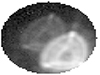 |
Fig. A.1. Imagette from CHEOPS. It shows the star being occulted by Triton in the center and the bright PSF of Neptune in the lower right corner. The peculiar shape of the PSF is due to the defocused optics of CHEOPS. The diameter of the imagette is 60 arcsecs, and the separation between Neptune and Triton varied between 18 and 15 arcsecs during the observation. |
The resulting imagette photometry clearly resolves the ingress and egress. The photometric noise is estimated by PIPE to increase from 0.5% to 0.9% per exposure during the 15 min centered on the occultation. This noise is mainly due to the photon-counting statistics and is dominated by scattered light from the nearby Neptune, with negligible contribution from the detector. The noise varies in time due to the asymmetric PSF of CHEOPS in combination with field rotation changing with time, which causes a variable contamination from the planet.
A.2. IAO observations
Successful observations were carried out at the Indian Astronomical Observatory (IAO), at the top of Mt. Saraswati, Digpa Ratsa Ri in Hanle, Ladakh, using the 2 m Himalayan Chandra Telescope (HCT) and the 0.7 m robotic GROWTH-India Telescope (GIT; Kumar et al. 2022). HCT recorded the event in the J band with the TIRSPEC instrument. It has a Teledyne 1024×1024 pixel Hawaii-1 PACE array with four quadrants, field of view (FoV) of 307″×307″, and plate scale of 0.3″per pixel. TIRSPEC offers the flexibility of subarray acquisition for faster readout (Ninan et al. 2014). For this event, a 307″×20″subarray was used to accommodate the target and the reference star in adjacent quadrants. The detector was readout nondestructively in the up-the-ramp (UTR) mode. The exposure time of each UTR cycle was 32 s, with dead times of 6.3 s between UTR cycles and integration time between consecutive nondestructive readout of 0.21 s. Dark and flat frames were obtained in the same configuration. Photometric calibration of the occulted star was carried out under similar observing conditions on 5 October 2022. However, with GIT, only the egress portion of the event could be captured. Observations were carried out in R band with the 4096 × 4108 pixel Andor iKon-XL 230 CCD camera, which has an FoV of 0.7°. The camera was operated in the fast-readout (1.0778 s) mode with an exposure time of 3 s.
For each frame of HCT and GIT observations, the photometric error was computed with PRAIA (Assafin 2023b) using a standard procedure based on the signal-to-noise ratio. Then, by calibrating the Triton flux using a close-by star, the flux ratio error was obtained from the propagated individual errors as 9% and 5% for HCT and GIT, respectively.
A.3. Yanqi Lake observation
For this observation, F. D. Romanov first contacted J. Y. Zhao, who sent an observation request to Yanqi Lake Observatory, pertaining to the University of Chinese Academy of Sciences (UCAS, Beijing, China). The event was successfully recorded at this station on behalf of F. D. Romanov, using the 0.7 m f/6.5 corrected Dall-Kirkham (PlaneWave CDK700) telescope equipped with an Andor iKon-L DZ936-BV CCD. The CCD was operated in the R band using the subsampling and fast-readout mode (5 MHz), with an exposure time of 1 s and a readout time of 0.8 s. Using the same approach as for the IAO observations, the flux ratio error was estimated to be about 4%.
Circumstances of the observations.
All Tables
Parameters of the occulted star and Triton, and results of the atmospheric fits.
All Figures
|
Fig. 1. Geometry of the 6 October 2022 stellar occultation by Triton. Upper panel: Dark blue lines (continued in red outside the Earth) delimit the predicted path of the Triton shadow on Earth on 6 October 2022. The shadow moves from right to left. The shadow centers (black dots) are spaced by one minute, and the larger black dot marks the geocentric closest approach near 14:39:46 UT (Table 1). Colors indicate stations at which the occultation was successfully detected. The blue arc shows the motion of the CHEOPS spacecraft during the event, while the red and green dots show Mt. Saraswati and Yanqi Lake, respectively. The white dots show the stations that were clouded out (see Table A.1). Lower panel: Reconstructed geometry of the occultation as seen in the sky plane. The J2000 celestial north (N) and east (E) directions and the scale are displayed in the upper right corner. The gray arrow near the equator shows the direction of rotation of the satellite. The (Neptune-facing) prime meridian is drawn as a thicker line than the other meridians, and the label S marks the south pole. The dotted circle indicates the layer in the Triton atmosphere that causes the half-light level (∼90 km altitude). The colored lines are the trajectories of the star relative to Triton (also known as occultation chords) as observed from various stations (see labels), and the black arrow indicates the direction of motion. The open circle is the predicted center of Triton, and the cross marks the actual center derived from the atmospheric fit. The offset between the two mainly stems from a correction of the Triton ephemeris. |
| In the text | |
|
Fig. 2. Simultaneous fits of the data by synthetic light curves. Upper panel: Best fit to the data, shown as blue lines, using a Triton surface pressure of psurf = 14.54 μbar and other parameters provided in Table 1. The residuals (observations minus model) are shown in green. The lower and upper dotted horizontal lines mark the zero flux and the average flux of Triton plus the star, respectively. Each light curve is normalized to the total flux of Triton plus the star and is plotted over a time interval of 6 minutes. The red tick marks indicate 14:41:40 UT. The HCT light curve was binned over five data points (1.05-second time resolution) for a better comparison with the other light curves. We note that a faint central flash is present in the Yanqi Lake light curve. The 1σ error bars are obtained with the PRAIA software, which accounts for the instrumental and photon noises, knowing that the error bars for the CHEOPS data points are dominated by photon noise (see Appendix A). They are not visible here because they are smaller than the plotted dots. Lower panel: χ2 map of the simultaneous fits. The 1σ and 3σ level curves are shown in green. |
| In the text | |
|
Fig. 3. Comparison of observations with VMT models. The figure shows the atmospheric pressure of Triton obtained from occultation measurements taken between 1989 and 2022 (see dates and values in Table 1). The red point is the result of the 6 October 2022 occultation (this work). It has been obtained using the same method as adopted by MO22 (black points). The green point (G95) is from the V2 RSS occultation of 25 August 1989 (Gurrola 1995). The blue points are O97, ground-based stellar occultation, 14 August 1995 (Olkin et al. 1997); E03, ground-based stellar occultation, 18 July 1997 (Elliot et al. 2000); E00, HST-based stellar occultation, 4 November 1997 (Elliot et al. 2003). It should be noted that MO22 analyzed the RSS data of August 1989 and the occultation data of July 1997 independently of Gurrola (1995) and Elliot et al. (2000), respectively. The vertical axes show the pressures at the reference radius 1400 km (left) and at the surface (right), assuming psurf/p1400 = 12.01 (see text). The lines are examples of VTM simulations by Bertrand et al. (2022). The dash-dotted line shows a model with the southern cap within 90°S–30°S and the northern cap within 45°N–90°N. The dotted line shows a case with the southern cap within 90°S–30°S and the northern cap within 60°N–90°. The dashed line shows another case with the southern cap within 90°S–30°S and no northern cap (volatile-free northern hemisphere). The solid line presents a simulation in which the N2 ice evolved freely over millions of years so that permanent and seasonal polar caps as well as local frost deposits can form self-consistently. In this simulation, the formation of thin seasonal N2 frosts is predicted in the current southern summer in the equatorial regions. None of the simulations fits the data satisfactorily. The dashed line accounts for the pressure increase of 1995–1997, but overestimates the pressures measured in 2017 and 2022. The dotted line marginally explains the increase of 1995–1997 and satisfactorily fits the 2022 measurement, but fails to explain the 2017 point. The dash-dotted line does not fit the increase of 1995–1997, while going through the 2017 point, but fails to explain the 2022 point. The solid line accounts for a basically constant pressure between 1989, 2017, and 2022, as well as the slight increases between 2017 and 2022. However, it is only marginally consistent with the 1995 result, and it does not account for the pressure surge of 1997. |
| In the text | |
|
Fig. A.1. Imagette from CHEOPS. It shows the star being occulted by Triton in the center and the bright PSF of Neptune in the lower right corner. The peculiar shape of the PSF is due to the defocused optics of CHEOPS. The diameter of the imagette is 60 arcsecs, and the separation between Neptune and Triton varied between 18 and 15 arcsecs during the observation. |
| In the text | |
Current usage metrics show cumulative count of Article Views (full-text article views including HTML views, PDF and ePub downloads, according to the available data) and Abstracts Views on Vision4Press platform.
Data correspond to usage on the plateform after 2015. The current usage metrics is available 48-96 hours after online publication and is updated daily on week days.
Initial download of the metrics may take a while.