| Issue |
A&A
Volume 682, February 2024
|
|
|---|---|---|
| Article Number | A168 | |
| Number of page(s) | 8 | |
| Section | The Sun and the Heliosphere | |
| DOI | https://doi.org/10.1051/0004-6361/202347623 | |
| Published online | 20 February 2024 | |
MHD modelling of coronal streamers and their oscillations⋆
1
Centre for Mathematical Plasma Astrophysics (CmPA), Department of Mathematics, KU Leuven, Celestijnenlaan 200B, 3001 Leuven, Belgium
e-mail: This email address is being protected from spambots. You need JavaScript enabled to view it.
2
SIDC – Royal Observatory of Belgium (ROB), Av. Circulaire 3, 1180 Brussels, Belgium
3
Institute of Physics, University of Maria Curie-Skłodowska, ul. Radziszewskiego 10, 20-031 Lublin, Poland
Received:
27
July
2023
Accepted:
9
November
2023
Abstract
Context. The present work investigates solar coronal dynamics in particular streamer waves. Streamer waves are transverse oscillations of the streamer stalk, often generated by the passage of a coronal mass ejection (CME). Recent observational studies infer that the streamer wave is an eigenmode of the streamer plasma slab and an excellent candidate for coronal seismology.
Aims. In the present work, we aim to numerically investigate the theoretical concepts of the physics and properties of streamer waves and to complement the observational statistical analysis of these events.
Methods. We used the magnetohydrodynamics (MHD) module of MPI-AMRVAC. An adaptive mesh refinement scheme was employed to achieve high resolution for the streamer structure. All the simulations were computed on the same base grid with the same numerical methods. We considered a dipole magnetic field on the Sun and a uniformly accelerating solar wind. We introduced a θ-velocity perturbation within our computational domain in the plane of a streamer to excite the transverse motion.
Results. A numerical model for the streamer wave phenomena was constructed in the framework of 2.5D MHD. We performed a parameter study and identified a sensitivity of the streamer dynamics to the background solar wind speed, the characteristics of the perturbation, and the input parameters for the model, such as temperature and magnetic field. We performed a statistical analysis and compared the obtained modelling results with the database of such events from observations from three different coronagraphs. We observed a narrow range of phase speeds and a correlation between wavelength and period. This is consistent with the observations and supports the idea that the streamer wave is an eigenmode of the streamer plasma slab. The measured phase speed is consistently significantly higher than the speed calculated from the measured period and wavelength. The simple fit, when the difference between these two speeds is exactly the background solar wind speed, only matches a small fraction of the data. The obtained results indicate that further investigation is required into the Doppler shift effect in the MHD theory for coronal seismology.
Key words: magnetohydrodynamics (MHD) / methods: numerical / Sun: corona / Sun: oscillations
Movie is available at https://www.aanda.org.
© The Authors 2024
 Open Access article, published by EDP Sciences, under the terms of the Creative Commons Attribution License (https://creativecommons.org/licenses/by/4.0), which permits unrestricted use, distribution, and reproduction in any medium, provided the original work is properly cited.
This article is published in open access under the Subscribe to Open model. This email address is being protected from spambots. You need JavaScript enabled to view it. to support open access publication.
1. Introduction
Streamers are large ray-like structures in the solar corona. They take the shape of an arch-like (or helmet-like) feature close to the Sun, narrowing to a very thin stalk of around 3° at 5 solar radii (R⊙) in projection on the plane of the sky, which can extend out up to 30 R⊙ (Koutchmy & Livshits 1992; Loucif & Koutchmy 1989). In the present work, we consider helmet streamers, in which closed magnetic flux connects two regions of different polarity. Above this closed flux system, a cusp forms, and the current sheet stretches out up to the heliospheric current sheet between the two open polar flux systems of opposite polarity. Generally, helmet streamers form above active regions and are quasi-stable structures that are observable for long periods, covering several solar rotations (Koutchmy 1971; Zhukov et al. 2008).
Of particular interest are the largest wave phenomena in the solar corona: streamer waves. These are transverse oscillations propagating outwards along the plasma sheet of the thin streamer stalk and decaying within a few periods or wavelengths (Chen et al. 2010; Feng et al. 2011). They are generated by the solar coronal dynamics; for example, a streamer wave can be excited by disturbances due to interaction with a coronal mass ejection (CME).
Streamer waves were first identified by Chen et al. (2010), who studied data from the Large Angle and Spectrometric Coronagraph (LASCO) on board the Solar and Heliospheric Observatory (SOHO; Brueckner et al. 1995). These authors used running difference images to extract the wave profiles of the streamer wave events and to determine the wave properties, such as their wavelength, period, phase speed, and amplitude. Chen et al. (2010) observed an increase in wavelength and a simultaneous decrease in phase speed over time. Analysis of the phase speed showed it has two contributions: the phase speed of the mode in the plasma rest frame and the speed of the background solar wind. This study was extended by Feng et al. (2011), where analysis of the LASCO data for Solar Cycle 23 enabled the authors to construct a database for observations of the streamer wave phenomena.
Streamer waves were further thoroughly studied by Decraemer et al. (2019). In the latter work, the authors studied 22 events, exploiting Solar Terrestrial Relations Observatory (STEREO) A and B COR2 data (Kaiser et al. 2008) and LASCO data, and thus determined the wavelength, period, and phase speed of the streamer waves. The statistical study showed a narrow range of phase speeds and a very poor correlation between the speed of the wave and the speed of the corresponding source CME, indicating that the speed is mainly determined by the physical properties of the streamer rather than by the triggering CME. A moderate correlation between period and wavelength was found. As a result, it was concluded that the streamer wave can be considered to be an eigenmode of the streamer plasma slab. This makes such waves good candidates for coronal seismology. Coronal seismology, which involves the combination of observations with theoretical studies, is a very powerful technique for diagnosing the plasma parameters of the coronal medium that cannot be measured directly (see reviews by De Moortel & Nakariakov 2012; Nakariakov & Kolotkov 2020). For example, the seismology study conducted by Chen et al. (2011) and Feng et al. (2011) allowed the authors to estimate the Alfvén speed profiles and the magnetic field strength under the assumption that the streamer wave can be interpreted as the fast kink body mode (Edwin & Roberts 1982). The dispersion relation that these latter authors developed for a plasma-slab configuration enabled Chen et al. (2011) and Feng et al. (2011) to connect the phase speed of the mode in the plasma rest frame and the Alfvén speed in the region outside of the plasma sheet (the external Alfvén speed) under the assumption that the infinitely thin current sheet does not influence the considered perturbation.
A more in-depth analysis of the dispersion relation for a streamer-slab-like configuration, where a non-uniform plasma slab and an alternating magnetic field were considered, was presented in Chapter 4 of Decraemer (2020). Consistently with similar numerical studies by Smith et al. (1997), Fruit et al. (2002) and Decraemer (2020) showed that the phase speed of the kink oscillation is approximately equal to the external Alfvén speed.
Decraemer et al. (2020) also proposed that seismology can be used to precisely determine the solar wind speed because of the Doppler shift in magnetohydrodynamics (MHD) wave theory (e.g. Goossens et al. 1992; Nakariakov et al. 1996). In Chen et al. (2010), Feng et al. (2011) and Decraemer et al. (2020) the measured speeds were found to be consistently significantly higher than the calculated speeds (proper phase speed of the wave), because of the Doppler shift, i.e. the contribution from the background solar wind. By combining the steamer wave speed obtained from the observations with the proper phase speed of the wave in the framework of well-developed streamer wave theory, we can estimate the solar wind speed. This seismology technique is an alternative to the currently used blob tracking (Sheeley et al. 1997; Wang et al. 2000), which is limited by the required assumption of exact equality between the blob speed and the solar wind speed.
The aim of the present work is to expand our knowledge of streamer waves through numerical modelling. We describe and demonstrate a model of a helmet streamer and observe the oscillation of the streamer stalk triggered by a velocity perturbation. Exploiting this model, we performed a parameter study to investigate the sensitivity of the streamer dynamics to the background solar wind speed, the implemented perturbation, and the input parameters for the model, such as temperature and magnetic field, and we present our findings. We investigate the properties of streamer waves and complement the statistical analysis of these events. We compare our modelling results with the observations of streamer wave events from Chen et al. (2010), Feng et al. (2011) and Decraemer et al. (2020). Finally, we discuss the consistency of the solar wind speed we estimate using coronal seismology with our model.
2. Method and numerical model
In the present work, we used MPI-AMRVAC (message passing interface–adaptive mesh refinement versatile advection code; Keppens et al. 2012; Porth et al. 2014; Xia et al. 2018) to construct a model of a helmet streamer in the framework of ideal magnetohydrodynamics (MHD). We consider a 2.5D spherical axisymmetric domain with the radial distance denoted by r, the polar angle by θ, and the azimuthal angle by ϕ. The inner radial boundary corresponds to the surface of the Sun, that is, 1 R⊙, and the outer boundary extends to 100 R⊙. The domain covers the entire region between the solar north and south poles, that is, θ ∈ [0, π].
The set of MHD equations is solved on a 2D logarithmically stretched grid, and so plasma quantities do not depend on the azimuthal angle ϕ, but the velocities and magnetic fields are calculated taking into account all three vector components.
To obtain a streamer structure of high resolution, we chose the AMR protocol with up to two additional levels of refinement to resolve the most important current-carrying structures. The criteria for the refinement or coarsening is based on the parameter c introduced in Karpen et al. (2012) and used also in Hosteaux et al. (2018) and Talpeanu et al. (2020, 2022):
 (1)
(1)
where Bt, n is the tangential component of magnetic field along the segment ln of contour C, which corresponds to a grid cell. The quantities in the numerator consequently represent: the magnitude of the electric current passing through the surface S of the contour C, and the result after applying Stokes theorem and its discrete form on the grid. The denominator is the total absolute value of all contributions of current. In our case, the mesh is refined when c > 0.03, and is coarsened if c < 0.01. Between these two values, there is no change in grid resolution when advancing from one time step to the next. In addition, to resolve the base of the streamer, the region close to the Sun below 4 R⊙ is refined with two additional levels, in the same way as in Talpeanu et al. (2020).
The MHD equations are treated using a two-step predictor–corrector-type scheme for temporal discretization and a second-order finite-volume scheme TVDLF (total variation diminishing Lax-Friedrichs) for spatial discretization (Tóth & Odstrcil 1996). For the latter, we use the most robust “minmod” slope limiter (Keppens et al. 2012) and a Courant–Friedrichs–Lewy (CFL) condition with “courantpar” = 0.5. Maintaining a divergence-free solution is ensured by the generalised Lagrange multiplier (GLM) method (Dedner et al. 2002), whereby an additional scalar variable is used to implement the mixed hyperbolic propagation and parabolic damping of magnetic field divergence.
We run all simulations on the same base grid using the same refinement strategy and numerical methods. This means that the differences between different simulation results are entirely due to the different input parameters.
We use a solar wind model implemented by the inclusion of gravity in the momentum equations and empirical heating and cooling source terms in the energy equation. The gravity is included as in Groth et al. (2000). The volumetric heating–cooling function introduced in Groth et al. (2000) and Manchester et al. (2004) and also used by Hosteaux et al. (2018) and Talpeanu et al. (2020, 2022) is of the following form:
![Mathematical equation: $$ \begin{aligned} Q = \rho q_0(T_0-T)\exp [-(r-1 R_\odot )^2/\sigma _0^2], \end{aligned} $$](/articles/aa/full_html/2024/02/aa47623-23/aa47623-23-eq2.gif) (2)
(2)
with radial distance (i.e. distance from the Sun) denoted by r(R⊙), mass density by ρ(kg m−3), volumetric heating amplitude by q0(ergs g−1 s−1 K−1), target temperature by T0(K), and heating scale height by σ0(R⊙). In contrast to Manchester et al. (2004), and the works that followed, we abandon the latitudinal dependence of T0 and σ0, that is, the bimodal structure of the wind, as we assume the slow solar wind regime to be large enough to encompass the streamer wave, and thus remove the necessity for a fast solar wind. We also aimed to simplify the convergence – and thus save computational resources – and avoid the numerical effects that complicate the analysis of the streamers. Therefore, in our study, q0 and σ0 are fixed to 106 ergs g−1 s−1 K−1 and 4.5 R⊙, respectively. The parameters T and T0 are used to control the background solar wind. The parameters were initially chosen to match a realistic solar wind speed at Earth. Based on these values, we consider three different solar wind regimes to identify the effect of the background on the streamer dynamics. Figure 1 shows the radial profiles in the equatorial plane of the three wind regimes inside (θ = 0°) and outside (θ = 5°) the streamer for the selected variants. The average solar wind speed is denoted by vS/M/FSW. In Fig. 1, the values of vS/M/FSW at 30 R⊙ (bold) and at 100 R⊙ are indicated. Here and below, we refer to the slow solar wind (SSW), which corresponds to T0 = 1.08 MK and vSSW = 260 km s−1, the medium solar wind (MSW), T0 = 1.50 MK and vMSW = 390 km s−1, and the fast solar wind (FSW), T0 = 3.40 MK and vFSW = 730 km s−1, regimes. The effects of these differences on the wave propagation and streamer properties are addressed in the following sections.
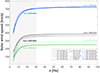 |
Fig. 1. 1D radial profiles in the equatorial plane for three solar wind regimes: SSW (green), MSW (grey), and FSW (blue) inside (dotted lines) and outside (solid lines) the streamer for the selected variants in the parameter study. The values of vS/M/FSW on the curves indicate the average solar wind speed within the regime at 30 R⊙ (bold) and at 100 R⊙. |
In our model, we consider a dipole magnetic field on the Sun with three different magnitudes of 1, 2, and 4 G at the poles, taken at the first cell of the domain.
The boundary conditions for the model are specified as follows. At the inner boundary, the density is fixed to 3.32 × 10⁻¹⁶ g cm−3; the temperature (T) is fixed to three different values: 1.32, 1.50, and 1.63 MK throughout the parameter study; the radial component of the momentum is extrapolated in the ghost cells, while the latitudinal and azimuthal components are set to zero. The term Brr2 is fixed at the inner boundary, while Bθ and Bϕ are extrapolated from the first inner cell. At the outer boundary, ρr2, T, ρr2vr, ρvθ, ρvϕ, Brr2, Bθ, and Bϕr are continuous.
3. Results: Helmet streamer
To perform the parameter study, we constructed 15 variants with different magnetic field strengths, temperatures and solar winds (see Fig. 3). The names of the variants were chosen according to the values of these parameters. The MSW variants are predominant, and so their names are not followed by an acronym, as in the case of SSW and FSW variants. Using the setup and the boundary conditions described in the previous section, we advanced our variants in time until reaching a steady state. As a result, a helmet streamer structure was obtained for all the variants. As an illustrative example, the resulting magnetic field configuration for the variant B1T1.50 is presented in Fig. 2.
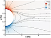 |
Fig. 2. Selected magnetic field lines and colour scale of the radial magnetic field Br in the meridional plane show the magnetic field configuration after reaching the steady-state solution for the variant B1T1.50. |
Key properties of the streamer waves for the simulation variants in the parameter study.
In the present work, we are exploring the possible effects of perturbations on streamer dynamics within a range of parameter sets rather than trying to reproduce realistic scenarios. It is believed that the streamers form in the slow solar wind environment and are not observed in the fast solar wind. However, FSW setup can result in a better understanding of the MHD Doppler shift effect. A more observational-data-driven setup will be the subject of a future study.
In Fig. 3, we present the logarithmic density distribution for all the studied variants. Let us first consider the nine variants in grey, which correspond to the MSW regime. We observe the following trends: An increase in magnetic field strength (within columns, lower rows correspond to higher magnetic field strengths) results in an expansion and lengthening of the streamer arcade, as well as in a more contrasted structure as density grows inside the streamer; an increase in temperature (within rows, the temperature increases from left right) results similarly in arcade expansion and lengthening and also in increasing width of the streamer stalk, with a smoother boundary. This behaviour can be explained by the changing balance between the magnetic and gas pressure. Thus, an increase in magnetic pressure leads to better plasma confinement inside the streamer, that is, a density increase, and an increase in gas pressure leads to more efficient plasma escape, and therefore a softer streamer boundary.
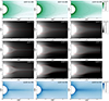 |
Fig. 3. Snapshots of the logarithmic number density (colour scale) and selected magnetic field lines for 15 variants in the parameter study. The green panels (top row) correspond to SSW, the grey panels (rows 2–4) to MSW; and the blue panels (bottom row) to FSW. The magnetic field strength increases from top to bottom within columns, and the temperature increases from left to right within rows. The colour scales are different for the different solar wind regimes. |
The green panels in Fig. 3 represent SSW solutions for a low magnetic field strength of 1 G and are to be compared with the upper row of grey panels. In the slow wind cases, we observe a streamer structure with a low contrast, a prolonged and expanded base, and a wide stalk.
The blue panels in Fig. 3 represent FSW solutions for high magnetic field of 4 G and are to be compared with the lower row of grey panels. We observe a small arcade and a narrow high-contrast streamer stalk.
Overall, all 15 variants demonstrate similar trends when varying the magnetic field strength or temperature. The change of the regime of the solar wind affects the density contrast inside and outside the streamer and the appearance of the streamer structure.
4. Results: Streamer wave
After a relaxation phase, the solar wind reaches a steady state and we then trigger transverse oscillation in the streamers by introducing a θ-velocity perturbation. After testing several cases, we conclude that the form of the perturbation does not affect the wave properties, in particular the phase speed. Therefore we chose a form that visually reproduces the wavy motion found in the observations:
![Mathematical equation: $$ \begin{aligned} v_{\rm pert} =s(r-a)\exp [-(r-a)^2/b^2], \end{aligned} $$](/articles/aa/full_html/2024/02/aa47623-23/aa47623-23-eq3.gif) (3)
(3)
where r(R⊙) is the distance from the Sun and the coefficients s(s−1), a(R⊙), and b(R⊙) determine the strength and the shape of the perturbation, where the parameter s is responsible for the amplitude of the perturbation and is fixed for all the variants to match the amplitude of around 0.1 R⊙ found in observations (Chen et al. 2010); the parameter a determines the radial location of the perturbation and is chosen to create a perturbation 1 R⊙ away from the cusp in order to not perturb the base of the streamer; and the parameter b determines the spatial size of the perturbation (i.e. the initial wavelength) and is chosen to match the angular velocity (around 30 km s−1) of the streamer deflection during the streamer wave event, estimated from observations (Decraemer et al. 2020). The perturbation is introduced in the plane of the streamer as a step function in the θ-direction, where θ ∈ [ − 5° ,5° ]. The resulting vθ distribution for the variant B1T1.50 is shown in Fig. 4, where a = 6.5 R⊙, s = 0.5 s−1, and  . The perturbation is applied as a right-hand side term in the momentum equation for Δt = 2 h. Subsequently, the system relaxes and we observe the wavy motion that propagates away from the Sun (i.e. to the right in the plots). The perturbation does not affect the streamer base.
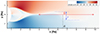 |
Fig. 4. 2D plot of the vθ(km s−1) distribution (colour scale) immediately after (t = 12 min) the introduction of the perturbation for the variant B1T1.50. The coefficients s, a, and b determine the strength and the shape of the perturbation. |
We started from the excitation of the waves with the wavelength λ = 6 R⊙, which corresponds to a mean wavelength found in the statistical study of Decraemer et al. (2020). Panels a–e in Fig. 5 present simulation snapshots 3 h after the introduction of the perturbation depicting the outward-propagating transverse oscillations of the streamers from the second column in Fig. 3. In our model we do not see any signature of the backward-propagating wave. This may be due to the location of the perturbation – mainly beyond the Alfvén surface, in the region where the local solar wind speed exceeds the local Alfvén speed. Thus, we expect to see the D’Alembert splitting of the wave front, with both fronts propagating outwards. The lack of a backward-propagating wave may also be attributed to the employed refinement strategy and highly diffusive numerical method with low CFL number (see Sect. 2). Panel f in Fig. 5 shows the STEREO A/COR2 white-light image of the streamer wave event 13 (Decraemer et al. 2020), identified on 2013 Feb. 6 from 00:24:00 to 06:24:00, at 02:39:00 (∼2 h after the start of the event) cropped to match the modelling data snapshots. The streamer properties for the modelled cases are determined and presented in the following section. The movie of the streamer wave events is available online.
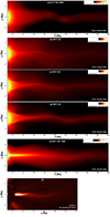 |
Fig. 5. Comparison of the simulation results with the observation. Panels a–e: Snapshots of the logarithmic density (colour scale) of the variants corresponding to the T = 1.50 K 3 h after introducing the perturbation. Panel f: STEREO A/COR2 white-light image of the streamer wave event on 2013 Feb. 6 at 02:39:00 (∼2 h after the start of the event). |
To expand our study, we also considered two additional s-values (i.e. initial wavelengths), namely 4.5 R⊙ and 8.5 R⊙. The corresponding variants B2T1.32W4.5 and B2T1.32W8.5 are based on the variant B2T1.32 and only differ by the initial wavelength. The discussed variants are compared in the following section.
Overall, the simulations reproduce the observations at least qualitatively. Despite the relatively small changes of the parameters in our study, we observe different streamer dynamics. We notice the most drastic differences in the amplitude of the oscillations and the phase speed of the wave when observed in different background solar wind regimes.
5. Statistical analysis of the simulated streamer waves and comparison with observations
After implementing the transverse oscillations for all the variants in the parameter study (excluding the variant B4T1.32, which shows poor convergence) for each individual event, we measured key properties, such as wavelength, period, and phase speed in the inertial frame of reference. We treat our modelling data in a similar way to the observations and exploit the methods as in Decraemer et al. (2020). We illustrate our measurements using the variant B1T1.50 as an example.
To measure the period of the modelled streamer wave events, we constructed a time–distance map along the green slit shown in panel a of Fig. 6. The slit intersects the streamer stalk at 12 R⊙. We consider the segment from –2 to 2 R⊙ and a time period of 800 min with a time resolution of 12 min. We then measure the half-period as the time between the trough and the crest, as shown in panel b of Fig. 6. All the values of the measured periods (P) are presented in the second column of Table 1.
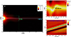 |
Fig. 6. Example of determining the streamer wave properties. Panel a shows a simulation snapshot of the logarithmic density, depicting the streamer wave event B1T1.50. Green and light-blue lines show the slits along which the time–distance maps were constructed to determine the streamer wave properties. The colour scale in (a) corresponds to the logarithmic density. Panel b shows the time–distance map along the green slit in panel a. The black arrow in panel b indicates the half period measurement for the variant B1T1.50 (168 min). The colour scale in (b) corresponds to the logarithmic density. Panel c shows the time–distance map along the light-blue slit in panel a. The blue line is the linear fit corresponding to the phase speed (392 km s−1). The colour scale in (c) corresponds to the θ-velocity. |
In agreement with the observations (Chen et al. 2010; Feng et al. 2011), we notice the growth of the wavelength and amplitude, which, in our model, is caused by the density distribution, that is, the density decreases as 1/r2. Panel a of Fig. 7 shows this growth for the five events in Fig. 5. For the statistical analysis, we consider the wavelength 3 h after the introduction of the perturbations. The wavelength is measured as a distance between two crests, as shown in panel b of Fig. 7. All wavelengths (λ) are presented in the third column of Table 1.
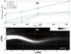 |
Fig. 7. Wavelength increase found in simulation. (a) Growth of the wavelength over time for the five variants corresponding to T = 1.50 MK. (b) Snapshot of the logarithmic density (colour scale) of the variant B1T1.50 3 h after the introduction of the perturbation, where we show how the wavelength was estimated. |
The measurements of the phase speed were performed using a time–distance map along the light-blue slit, as shown in panel a of Fig. 6. The slit is built along the streamer stalk and covers the interval from 1 to 30 R⊙. We fit a linear profile to the points corresponding to the maximum value of the θ-velocity within each time step, as shown in panel c of Fig. 6. Thus, the linearly fitted speed is considered as our measured phase speed. All the values of the measured phase speeds (vph) are presented in the fourth column of Table 1.
In order to estimate the Doppler effect, we calculated the proper phase speed of the mode also using the simple formula λ/P. The results are presented in the fifth column of Table 1.
Further, we performed a statistical study of the modelling results and compare our findings with the observations. To this end, we consider 16 simulations and two sets of observational data with a total of 24 events. We use the parameters of the 22 events from Table 1 in Decraemer et al. (2020). We also use the events 20030605 and 20040706 (or the event W, studied also in Chen et al. 2010, 2011) from Feng et al. (2011), for which the wave properties were precisely measured. The periods and the wavelengths of these events were taken at 4 R⊙ (see Fig. 8 in Feng et al. 2011). The phase speeds correspond to the first phase – P1 (see Fig. 8 in Feng et al. 2011 and Fig. 1 in Chen et al. 2011), which were also measured at 4 R⊙. These parameters are presented in Table 2.
Streamer wave parameters from the observational database.
The scatter plot in Fig. 8 shows a comparison of the wavelength with the period measurements. The Pearson correlation coefficient of the two quantities is 0.68 for the 24 observations (the red line) and 0.83 for the simulations (the maroon line). In agreement with the observations, the simulations also show a strong correlation between wavelength and period. These results support the idea that the streamer wave is an eigenmode of the streamer slab.
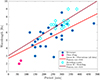 |
Fig. 8. Scatter plot of period vs. wavelength for the streamer wave events from observational studies and from our simulations. Blue circles correspond to the events from Decraemer et al. (2020) and magenta circles correspond to the events from Table 2. Turquoise diamonds correspond to the modelling results. The linear regression line fits to the data are shown in red (observations) and maroon (modelling). |
In Fig. 9, we present the relation between the calculated phase speeds λ/P and the measured phase speeds vph. The red line corresponds to equal values of the calculated and the measured speeds. Thus, in simulations as well as in the observations, the measured speeds are consistently significantly higher than the calculated speeds. As the streamer waves are propagating in an already moving medium, we observe the Doppler shift known from MHD wave theory, where there are two contributions to the measured phase speed: the proper phase speed of the wave and the background solar wind speed.
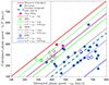 |
Fig. 9. Scatter plot of measured phase speed (vph) vs. calculated speed (λ/P) for the streamer wave events from observational studies and from simulations. Blue circles correspond to the events from Decraemer et al. (2020) and magenta circles correspond to the events from Table 2. Diamonds correspond to the modelling results, where green diamonds represent SSW variants, grey diamonds represent MSW variants, and blue diamonds represent FSW variants. The red line marks the equal values of the calculated and measured phase speed. The blue dashed line corresponds to a fit with a constant solar background wind (averaged difference between vph and λ/P). Solid lines correspond to the fit λ/P = vph − vSW, where vSW represents the averaged solar wind speed estimated from the observations or calculated from the modelling setup. Dotted lines correspond to the fit λ/P = vph − αvSW, where αvSW represents the averaged difference between vph and λ/P. |
In Fig. 9, we also present the fit to the observational data and to the modelling introduced in Decraemer et al. (2020). The fit in the form λ/P = vph − vSW corresponds to a forward propagating wave and was used to estimate the solar wind speed. Here, the dashed blue line corresponds to the background solar wind 298 km s−1 under the assumption that it is the same for all 22 streamer wave events (denoted “Decraemer” in Fig. 9) and is calculated by taking the average difference between the calculated phase speeds (λ/P) and the measured phase speeds (vph).
If we take the known (estimated from the observations and implemented in the model) solar wind speed, this fit seems to match the two observations (denoted “Chen+Feng” in Fig. 9), but not the modelling data. Thus, the solid magenta line corresponds to the average (in the interval 1–10 R⊙) solar wind speed of 120 km s−1 estimated from the observations (Sheeley et al. 1997; Wang et al. 2000). However, for these events, the measurements are taken in the region of comparatively slow solar wind, and the Doppler shift effect may be less significant. The solid green, grey, and blue lines correspond to the average (in the interval 1–30 R⊙, see Fig. 1) values of solar wind speed in our parameter study: vSSW = 160 km s−1, vMSW = 255 km s−1, and vFSW = 540 km s−1.
A better match to the modelling data is provided by the fit λ/P = vph − αvSW, shown by the dashed green, grey, and blue lines. The term αvSW corresponds to the average difference between the calculated phase speeds (λ/P) and the measured phase speeds (vph). The quantity vS/M/FSW is as discussed in the previous paragraph. The correcting factor α varies between 0.35 and 0.67.
Overall, this indicates that further investigation is required into the theory of the MHD Doppler shift effect in the streamer waves and the wave properties. For example, there is a discrepancy in terms of using both locally measured and average values. To extend the analysis of the simulations, additional slits could be used to estimate the periods and the phase speeds of the wave at different heliocentric distances. This would also allow us to perform a seismological study similar to those of Chen et al. (2011) and Feng et al. (2011), where the Alfvén speed and the magnetic field profiles are deduced from the phase speed of the mode in the plasma rest frame. These profiles could be compared to the ones calculated directly from the model, which would allow us to estimate the reliability of and to improve the seismological approach. This is a prospect for a future study.
Another possibility is that the discrepancy with the original fit might be caused by lost physical effects due to simplifications made in our model; in particular, our choice to abandon the bi-modal structure of the solar wind. In addition to the Doppler shift effect arising in the case of a homogeneous flow, in the presence of an inhomogeneous flow, it may be important to consider the appearance of the negative energy wave phenomena and the change of the dispersion characteristics of the wave (Nakariakov & Roberts 1995). Indeed, the fast magnetoacoustic body modes in solar wind might be subject to the negative energy wave instabilities (Joarder et al. 1997; Andries & Goossens 2002). These effects are out of the scope of our current model. The construction of a model with more realistic solar wind conditions will form part of our future research.
6. Conclusions
We constructed a numerical model of a helmet streamer using the MHD module of MPI-AMRVAC and an AMR protocol to resolve the streamer structure. Based on this model, we performed a parameter study to identify the sensitivity of the streamer dynamics to the magnetic field, temperature, and background solar wind. We propose a simple excitation mechanism for a streamer wave, where the wavy motions of the streamer stalk are triggered by the introduction of a vθ perturbation in the plane of the streamer. We performed 16 simulations in total. Overall, the simulations qualitatively reproduce the observations.
We measured the period, wavelength, and phase speed for each streamer wave event. We observe a narrow range of phase speeds and a correlation between wavelength and period. This is consistent with observational studies and supports the idea that the streamer wave is an eigenmode of the streamer plasma slab. We also observed another effect found in the observations: the measured speeds are consistently significantly higher than the calculated speeds. We analysed the difference between the two quantities and show that the simple fit, where the measured speed is the linear sum of the proper speed of the wave and the background solar wind, does not approximate the modelling data well. This discrepancy may be caused by the measurement methodology and the physical effects lost due to simplifications made in our model. Overall, further investigation is needed into the Doppler shift effect in MHD theory for seismology. We plan to carry out a more in-depth analysis of the streamer wave properties, in particular the phase speed and its relation to the sound speed and Alfvén speed.
Future research will also include the construction of a 3D model with realistic solar wind conditions and magnetic field configuration, where we will accurately reproduce a streamer wave event taking into account recent observational and numerical advances.
Movie
Movie 1 associated with Fig. 5 (Fig5_video) Access Supplementary Material
Acknowledgments
The work was funded by the European Research Council (ERC) under the European Union’s Horizon 2020 research and innovation program (grant agreement No. 724326) and the C1 grant TRACEspace of Internal Funds KU Leuven. For the computations we used the infrastructure of the VSC “Flemish Supercomputer Center, funded by the Hercules foundation and the Flemish Government” department EWI. S.P. acknowledges support from the projects C14/19/089 (C1 project Internal Funds KU Leuven), G.0B58.23N and G.0025.23N (FWO-Vlaanderen), SIDC Data Exploitation (ESA Prodex-12), and Belspo project B2/191/P1/SWiM.
References
- Andries, J., & Goossens, M. 2002, Phys. Plasmas, 9, 2876 [NASA ADS] [CrossRef] [Google Scholar]
- Brueckner, G. E., Howard, R. A., Koomen, M. J., et al. 1995, Sol. Phys., 162, 357 [NASA ADS] [CrossRef] [Google Scholar]
- Chen, Y., Song, H. Q., Li, B., et al. 2010, ApJ, 714, 644 [NASA ADS] [CrossRef] [Google Scholar]
- Chen, Y., Feng, S. W., Li, B., et al. 2011, ApJ, 728, 147 [NASA ADS] [CrossRef] [Google Scholar]
- Decraemer, B. 2020, Ph.D. Thesis, KU Leuven, Belgium [Google Scholar]
- Decraemer, B., Zhukov, A., & Van Doorsselaere, T. 2019, ApJ, 883, 152 [NASA ADS] [CrossRef] [Google Scholar]
- Decraemer, B., Zhukov, A., & Van Doorsselaere, T. 2020, ApJ, 893, 78 [NASA ADS] [CrossRef] [Google Scholar]
- Dedner, A., Kemm, F., Kröner, D., et al. 2002, J. Comput. Phys., 175, 645 [Google Scholar]
- De Moortel, I., & Nakariakov, V. M. 2012, ApJ, 370, 3193 [Google Scholar]
- Edwin, P. M., & Roberts, B. 1982, Sol. Phys., 76, 239 [Google Scholar]
- Feng, S. W., Chen, Y., Li, B., et al. 2011, Sol. Phys., 272, 119 [NASA ADS] [CrossRef] [Google Scholar]
- Fruit, G., Louarn, P., Tur, A., & Le QuéAu, D. 2002, J. Geophys. Res.: Space Phys., 107, 1411 [NASA ADS] [Google Scholar]
- Goossens, M., Hollweg, J. V., & Sakurai, T. 1992, Sol. Phys., 138, 233 [Google Scholar]
- Groth, C. P. T., De Zeeuw, D. L., Gombosi, T. I., & Powell, K. G. 2000, J. Geophys. Res., 105, 25053 [NASA ADS] [CrossRef] [Google Scholar]
- Hosteaux, S., Chané, E., Decraemer, B., Talpeanu, D. C., & Poedts, S. 2018, A&A, 620, A57 [NASA ADS] [CrossRef] [EDP Sciences] [Google Scholar]
- Joarder, P. S., Nakariakov, V. M., & Roberts, B. 1997, Sol. Phys., 176, 285 [NASA ADS] [CrossRef] [Google Scholar]
- Kaiser, M. L., Kucera, T. A., Davila, J. M., et al. 2008, Space Sci. Rev., 136, 5 [Google Scholar]
- Karpen, J. T., Antiochos, S. K., & DeVore, C. R. 2012, ApJ, 760, 81 [NASA ADS] [CrossRef] [Google Scholar]
- Keppens, R., Meliani, Z., van Marle, A., et al. 2012, J. Comput. Phys., 231, 718 [Google Scholar]
- Koutchmy, S. 1971, A&A, 13, 79 [NASA ADS] [Google Scholar]
- Koutchmy, S., & Livshits, M. 1992, Space Sci. Rev., 61, 393 [CrossRef] [Google Scholar]
- Loucif, M. L., & Koutchmy, S. 1989, A&AS, 77, 45 [NASA ADS] [Google Scholar]
- Manchester, W. B., IV, Gombosi, T. I., Roussev, I., et al. 2004, J. Geophys. Res.: Space Phys., 109, 2107 [NASA ADS] [Google Scholar]
- Nakariakov, V. M., & Kolotkov, D. Y. 2020, ARA&A, 58, 441 [Google Scholar]
- Nakariakov, V. M., & Roberts, B. 1995, Sol. Phys., 159, 213 [NASA ADS] [CrossRef] [Google Scholar]
- Nakariakov, V. M., Roberts, B., & Mann, G. 1996, A&A, 311, 311 [NASA ADS] [Google Scholar]
- Porth, O., Xia, C., Hendrix, T., Moschou, S. P., & Keppens, R. 2014, ApJS, 214, 4 [Google Scholar]
- Sheeley, N. R., Jr., Wang, Y. M., Hawley, S. H., et al. 1997, ApJ, 484, 472 [NASA ADS] [CrossRef] [Google Scholar]
- Smith, J. M., Roberts, B., & Oliver, R. 1997, A&A, 327, 377 [NASA ADS] [Google Scholar]
- Talpeanu, D.-C., Chané, E., Poedts, S., et al. 2020, A&A, 637, A77 [NASA ADS] [CrossRef] [EDP Sciences] [Google Scholar]
- Talpeanu, D.-C., Poedts, S., D’Huys, E., & Mierla, M. 2022, A&A, 658, A56 [NASA ADS] [CrossRef] [EDP Sciences] [Google Scholar]
- Tóth, G., & Odstrcil, D. 1996, J. Comput. Phys., 128, 82 [CrossRef] [Google Scholar]
- Wang, Y. M., Sheeley, N. R., Socker, D. J., Howard, R. A., & Rich, N. B. 2000, Geophys. Res. Lett., 105, 25133 [NASA ADS] [CrossRef] [Google Scholar]
- Xia, C., Teunissen, J., Mellah, I. E., Chané, E., & Keppens, R. 2018, ApJS, 234, 30 [NASA ADS] [CrossRef] [Google Scholar]
- Zhukov, A. N., Saez, F., Lamy, P., Llebaria, A., & Stenborg, G. 2008, ApJ, 680, 1532 [NASA ADS] [CrossRef] [Google Scholar]
All Tables
Key properties of the streamer waves for the simulation variants in the parameter study.
All Figures
|
Fig. 1. 1D radial profiles in the equatorial plane for three solar wind regimes: SSW (green), MSW (grey), and FSW (blue) inside (dotted lines) and outside (solid lines) the streamer for the selected variants in the parameter study. The values of vS/M/FSW on the curves indicate the average solar wind speed within the regime at 30 R⊙ (bold) and at 100 R⊙. |
| In the text | |
|
Fig. 2. Selected magnetic field lines and colour scale of the radial magnetic field Br in the meridional plane show the magnetic field configuration after reaching the steady-state solution for the variant B1T1.50. |
| In the text | |
|
Fig. 3. Snapshots of the logarithmic number density (colour scale) and selected magnetic field lines for 15 variants in the parameter study. The green panels (top row) correspond to SSW, the grey panels (rows 2–4) to MSW; and the blue panels (bottom row) to FSW. The magnetic field strength increases from top to bottom within columns, and the temperature increases from left to right within rows. The colour scales are different for the different solar wind regimes. |
| In the text | |
|
Fig. 4. 2D plot of the vθ(km s−1) distribution (colour scale) immediately after (t = 12 min) the introduction of the perturbation for the variant B1T1.50. The coefficients s, a, and b determine the strength and the shape of the perturbation. |
| In the text | |
|
Fig. 5. Comparison of the simulation results with the observation. Panels a–e: Snapshots of the logarithmic density (colour scale) of the variants corresponding to the T = 1.50 K 3 h after introducing the perturbation. Panel f: STEREO A/COR2 white-light image of the streamer wave event on 2013 Feb. 6 at 02:39:00 (∼2 h after the start of the event). |
| In the text | |
|
Fig. 6. Example of determining the streamer wave properties. Panel a shows a simulation snapshot of the logarithmic density, depicting the streamer wave event B1T1.50. Green and light-blue lines show the slits along which the time–distance maps were constructed to determine the streamer wave properties. The colour scale in (a) corresponds to the logarithmic density. Panel b shows the time–distance map along the green slit in panel a. The black arrow in panel b indicates the half period measurement for the variant B1T1.50 (168 min). The colour scale in (b) corresponds to the logarithmic density. Panel c shows the time–distance map along the light-blue slit in panel a. The blue line is the linear fit corresponding to the phase speed (392 km s−1). The colour scale in (c) corresponds to the θ-velocity. |
| In the text | |
|
Fig. 7. Wavelength increase found in simulation. (a) Growth of the wavelength over time for the five variants corresponding to T = 1.50 MK. (b) Snapshot of the logarithmic density (colour scale) of the variant B1T1.50 3 h after the introduction of the perturbation, where we show how the wavelength was estimated. |
| In the text | |
|
Fig. 8. Scatter plot of period vs. wavelength for the streamer wave events from observational studies and from our simulations. Blue circles correspond to the events from Decraemer et al. (2020) and magenta circles correspond to the events from Table 2. Turquoise diamonds correspond to the modelling results. The linear regression line fits to the data are shown in red (observations) and maroon (modelling). |
| In the text | |
|
Fig. 9. Scatter plot of measured phase speed (vph) vs. calculated speed (λ/P) for the streamer wave events from observational studies and from simulations. Blue circles correspond to the events from Decraemer et al. (2020) and magenta circles correspond to the events from Table 2. Diamonds correspond to the modelling results, where green diamonds represent SSW variants, grey diamonds represent MSW variants, and blue diamonds represent FSW variants. The red line marks the equal values of the calculated and measured phase speed. The blue dashed line corresponds to a fit with a constant solar background wind (averaged difference between vph and λ/P). Solid lines correspond to the fit λ/P = vph − vSW, where vSW represents the averaged solar wind speed estimated from the observations or calculated from the modelling setup. Dotted lines correspond to the fit λ/P = vph − αvSW, where αvSW represents the averaged difference between vph and λ/P. |
| In the text | |
Current usage metrics show cumulative count of Article Views (full-text article views including HTML views, PDF and ePub downloads, according to the available data) and Abstracts Views on Vision4Press platform.
Data correspond to usage on the plateform after 2015. The current usage metrics is available 48-96 hours after online publication and is updated daily on week days.
Initial download of the metrics may take a while.