| Issue |
A&A
Volume 682, February 2024
|
|
|---|---|---|
| Article Number | A27 | |
| Number of page(s) | 15 | |
| Section | Astronomical instrumentation | |
| DOI | https://doi.org/10.1051/0004-6361/202346660 | |
| Published online | 30 January 2024 | |
The Bi–O edge wavefront sensor
How Foucault-knife-edge variants can boost extreme adaptive optics
1
European Southern Observatory (ESO),
Karl Schwarzschild-str 2,
85748
Garching-bei-Muenchen,
Germany
e-mail: This email address is being protected from spambots. You need JavaScript enabled to view it.
2
DOTA, ONERA,
13661
Salon Cedex Air,
France
3
Aix-Marseille Univ, CNRS, CNES, LAM,
13388
Marseille,
France
4
Centre de Recherche Astrophysique de Lyon (CRAL),
9 avenue Charles André,
69230
Saint Genis-Laval,
France
Received:
14
April
2023
Accepted:
9
August
2023
Abstract
Context. Direct detection of exoplanets around nearby stars requires advanced adaptive optics (AO) systems. High-order systems are needed to reach a high Strehl ratio (SR) in near-infrared and optical wavelengths on future giant segmented-mirror telescopes (GSMTs). Direct detection of faint exoplanets with the European Southern Observatory (ESO) Extremely Large Telescope (ELT) will require some tens of thousands of correction modes. The resolution and sensitivity of the wavefront sensor (WFS) are key requirements for this science case. We present a new class of WFSs, the bi-orthogonal Foucault knife-edge sensors (or Bi–O edge), that is directly inspired by the Foucault knife-edge test. The idea consists of using a beam-splitter producing two foci, each of which is sensed by an edge with a direction orthogonal to the other focus.
Aims. We describe two implementation concepts: The Bi–O edge sensor can be realised with a sharp edge and a tip-tilt modulation device (sharp Bi–O edge) or with a smooth gradual transmission over a grey edge (grey Bi–O edge). A comparison of the Bi–O edge concepts and the four-sided classical pyramid wavefront sensor (PWS) gives some important insights into the nature of the measurements.
Methods. We analytically computed the photon noise error propagation, and we compared the results to end-to-end simulations of a closed-loop AO system.
Results. Our analysis shows that the sensitivity gain of the Bi–O edge with respect to the PWS depends on the system configuration. The gain is a function of the number of control modes and the modulation angle. We found that for the sharp Bi–O edge, the gain in reduction of propagated photon noise variance approaches a theoretical factor of 2 for a large number of control modes and small modulation angle, meaning that the sharp Bi–O edge only needs half of the photons of the PWS to reach similar measurement accuracy. In contrast, the PWS is twice more sensitive than the Bi–O edge in the case of very low order correction and/or large modulation angles. Preliminary end-to-end simulations illustrate some of the results. The grey version of the Bi–O edge opens the door to advanced amplitude filtering, which replaces the need for a tip-tilt modulator while keeping the same dynamic range. We show that an additional factor of 2 in reduction of propagated photon noise variance can be obtained for high orders, such that the theoretical maximum gain of a factor of 4 in photon efficiency can be obtained. A diffractive Fourier model that accurately includes the effect of modulation and control modes shows that for the extreme AO (XAO) system configuration of the ELT, the overall gain will well exceed one magnitude in guide-star brightness when compared to the modulated PWS.
Conclusions. We conclude that the Bi–O edge is an excellent candidate sensor for future very high order Adaptive Optics systems, in particular on GSMTs.
Key words: instrumentation: adaptive optics / methods: analytical / instrumentation: high angular resolution / planetary systems / methods: numerical
© The Authors 2024
 Open Access article, published by EDP Sciences, under the terms of the Creative Commons Attribution License (https://creativecommons.org/licenses/by/4.0), which permits unrestricted use, distribution, and reproduction in any medium, provided the original work is properly cited.
This article is published in open access under the Subscribe to Open model. This email address is being protected from spambots. You need JavaScript enabled to view it. to support open access publication.
1 Introduction
High-contrast direct imaging (HCI) of exoplanets from the ground is one of the most demanding applications of adaptive optics (AO). Current HCI instruments such as the Spectro-Polarimetric High-contrast Exoplanet REsearch (SPHERE; Beuzit et al. 2019), the GEMINI Planet Imager (GPI; Macintosh et al. 2018), the SUBARU Coronagraphic Extreme Adaptive Optics (SCExAO; Jovanovic et al. 2015), the Keck Planet Imager and Characterizer (KPIC; Mawet et al. 2018), or the Magellan extreme AO system (MagAO-X Males et al. 2018) installed on 8m class telescopes, reach high-contrast sensitivities, which led to the discovery of several young giant planets (e.g. Macintosh et al. 2015; Keppler et al. 2018; Lagrange et al. 2010). The direct-imaging method has also allowed powerful characterisation of the planetary atmospheres through direct spectroscopy, returning not only effective temperatures and surface gravities, but also detections of molecular species that provide basic estimates of the compositions of the atmosphere (e.g. Konopacky et al. 2013).
A main achievement of exoplanetary science in the past several years is the determination that low-mass planets are common (Dressing & Charbonneau 2013), and the identification of numerous more such objects is expected to proceed in the coming years. The new generation of giant 30 to 40 m class telescopes (the Extremely Large Telescope (ELT), the Giant Magellan Telescope (GMT), and the Thirty Meter Telescope (TMT)) in the 2030s is expected to be capable of detecting and characterising these small planets with sizes of Earth to sub-Neptunes around the closest M dwarfs even when they are located in the habitable zone (Kasper et al. 2021).
The HCI instruments typically combine extreme AO (XAO; Guyon 2005), coronagraphy (Mawet et al. 2012), and quasi-static speckle control (e.g. Give’on et al. 2007) as well as advanced post-processing (e.g. Marois et al. 2006; Hoeijmakers et al. 2018). These concepts promise to effectively reduce speckle noise to the level at which instruments are limited by the photon noise of the XAO residual halo of the coronagraphic point spread function (PSF).
In HCI limited by photon noise, the observing time is proportional to the square of the signal-to-noise ratio (S/N). Because the latter is proportional to the Strehl ratio (SR), it becomes critical for HCI to maximise the SR and minimise the residual halo over the control radius of the XAO deformable mirror (DM).
For instance, the SPHERE instrument was designed to detect exoplanets with atmospheres containing methane at the 1.65 µm absorption feature in the H band. To do this, the primary top-level requirement of SPHERE XAO, SAXO (Fusco et al. 2014), is to reach an almost perfect light concentration in the core of the PSF at the observing wavelength with an SR of 90% in the H band. This was achieved by setting the resolution of the sensor to a 20 cm sampling of the telescope aperture. The ultimate goal of the ELT Planetary Camera Spectrograph (PCS; Kasper et al. 2021) is to detect bio-markers in the atmosphere of exo-planets, for example, the A band of molecular oxygen at around 760 nm. A high SR becomes more difficult to reach at shorter wavelengths and will ultimately be limited by the DM fitting error. The PCS XAO system must therefore push AO to its limits, and this calls for the most sensitive wavefront sensor (WFS) in order to minimise the residual halo.
In this paper, we revisit the concept of the two sided pyramid WFS proposed by Phillion & Baker (2006). We generalise the concept and propose new optical implementations. To underline the nature of the focal plane elements, we name the concept the bi-orthogonal Foucault knife-edge sensor (short name: Bi–O edge). We compare its properties to a reference, the well-known pyramid wavefront sensor (PWS) (Ragazzoni 1996). This sensor is now well established, with many systems producing science on sky, for instance, at the Large Binocular Telescope (Esposito et al. 2013), on SUBARU (Jovanovic et al. 2015), the Keck telescope (Bond et al. 2020), the Magellan Clay Telescope (Males et al. 2018), and projects in development for the ELT (e.g. Clénet et al. 2018; Bertram et al. 2018; Schwartz et al. 2020) and the TMT (Crane et al. 2018).
After the presentation of the wave-front sensing context in Sect. 2, we analyse the Fourier filtering properties of a Foucault knife edge (FKE) in Sect. 3. The two flavours of Bi–O edge (sharp and grey) are presented in Sect. 4. In Sect. 5, we use the FKE properties to derive the PWS and Bi–O edge sensitivities and noise propagation. In Sect. 6, we use a modal approach to compare the performance for both Bi–O edge and PWS more accurately and show the dependence on the number of corrected modes as well as closed-loop simulations obtained with end-to-end models. A Fourier model for the Fourier-filtering WFS (FF-WFS) is given in Appendix A. This model is called the convolutional model (C model hereafter) and is used for the analytical developments presented in this paper.
2 Wave-front sensing context
The WFS is an essential part of an astronomical AO system. The increasing needs for high precision, high sensitivity, and a very large number of degrees of freedom (DoF) calls for a careful study of the WFS properties. During the early days of AO, the Lateral Shearing Interferometer (LSI) was the most commonly used sensor (Rousset 1999). It is interesting to note that this slope sensor required two channels, as the Bi–O edge does, one for each orthogonal wave-front derivative component.
Since ADONIS, the first workhorse astronomical AO instrument (Beuzit et al. 1997), the Shack-Hartmann Sensor (SHS) became the most frequently used WFS in AO. The success of the SHS was largely based on its conceptual simplicity, achromaticity, and wide linear range (Rousset 1999). In contrast to the LSI, the SHS maximised the flux sensitivity and simplified the opto-mechanical concept.
The PWS (Ragazzoni 1996) represented a giant leap in sensitivity at the expense of a slightly higher complexity and shorter dynamic range compared to the SHS. To cope with the issues of dynamic range, the PWS sensor is generally coupled to a tip-tilt (TT) modulated mirror that allows improving the linear range at the cost of some sensitivity. The sensitivity gain of the PWS over the SHS can be tremendous for high-order systems and was studied extensively (see Ragazzoni & Farinato 1999; Esposito & Riccardi 2001; Vérinaud et al. 2005; Guyon 2005).
The class of FF-WFS is a generalisation of the PWS concept that was first introduced and studied by Fauvarque et al. (2016). Using a few hypotheses, a theoretical formalism based on a C model has been developed and allows one to derive analytical transfer functions (TFs) depending on the filtering mask property.
Throughout this study, the PWS, as the most common FF-WFS (see Fig. 1), is used as a reference for the exploration of the Bi–O edge properties. Only circularly modulated PWSs are considered. While the PWS can be operated without modulation (e.g. Costa 2005; Nousiainen et al. 2022; Agapito 2023), the very short linear range of the non-modulated PWS makes it hard to operate in practice.
Interestingly, slope sensor concepts based on two channels with focal amplitude masks have been proposed (e.g. Horwitz 1994; Oti et al. 2005; Haffert 2016; Hénault et al. 2020) and share some practical implementation solutions with one of the variants of the Bi–O edge presented in this paper. In general, WFSs can be categorised into two families: the geometric and the diffractive WFSs. Geometric WFSs are characterised by a wide dynamic range and low sensitivity (the SHS), while the diffractive WFSs like the PWS offer high sensitivity, but are usually associated with a shorter dynamic range. The optimum choice depends on the scientific objective of the AO system. In this paper, we propose to study the Bi–O edge, a diffractive WFS concept offering unprecedented sensitivity for high-contrast XAO.
 |
Fig. 1 Schematic view of the concept of a modulated PWS sensor with a refractive pyramidal prism. A TT modulation mirror moves the focal spot over a four-facet pyramid. The signal is obtained by integrating the intensity on a pupil-plane detector during a modulation cycle. |
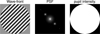 |
Fig. 2 Focal (centre) and pupil-plane (right) images corresponding to a purely spatial frequency wave-front (left). |
3 Foucault knife edge as a Fourier-filtering sensor
The FKE test (Foucault 1859) is commonly used in astronomy to quantify the radius of the curvature of optical devices by masking part of the ray-light in a pre- and post-focal plane. From a wave-front sensing perspective, if the mask is located in the focal plane, it can be seen as the most elementary FF-WFS. Vérinaud (2004) used a mono-dimensional model of a TT modulated FKE as a simplified model of the PWS. In this section, we generalise this model to two dimensions in order to highlight some remarkable properties.
3.1 Nature of the measurements of a Foucault knife edge
We consider a purely sinusoidal aberration with a standard deviation σϕ as a test wave-front with spatial frequency w0, and let r be the variable along the sinusoidal function axis. We define the measurement as the meta-intensity mI, which is a linear combination of pupil-intensity maps (from which null wavefront (WF) reference maps are subtracted). The sensitivity χmI in the small-phase regime is given by (Fauvarque et al. 2016)
 (1)
(1)
where || ⋅ ||2 is the L2 norm. In the small-phase regime, this WF creates two symmetric speckles in the focal plane at a distance from the core that depends on the spatial frequency (Malbet et al. 1995). The spatial frequency is chosen to be high enough to separate the speckles from the PSF core, as illustrated in Fig. 2. In the corresponding pupil plane, a uniform pupil is visible with an intensity I0 that corresponds to the square modulus of the electromagnetic field. In this situation, both speckles interfere with the core of the PSF, but the resulting interference fringes mask each other’s impact in the pupil plane.
When an amplitude mask is now added in the focal plane to mask one of the two speckles, as illustrated in Fig. 3, it causes a filtering of one of the satellite speckles. This operation allows us to reveal the interference pattern between the non-masked speckle with an intensity Ispeckle and the core of the PSF with an intensity Icore.
The resulting fringe amplitude  is
is
 (2)
(2)
The magnitude and phase of the fringes correspond to the Hilbert transform (Correia et al. 2020) of the incoming wave-front (±π/2 dephasing depending on which speckle interferes). In the small-phase regime, we can approximate the intensity in the core and the intensity in one speckle with
 (3)
(3)
We can express the meta-intensity corresponding to the core-speckle (CS) interference as
 (4)
(4)
Noting that  , and keeping only the first order in σϕ, we find that ||mICS(ϕ)||2 = σϕ.
Hence, the sensitivity corresponding to the CS meta-intensity is
 (5)
(5)
In Sect. 5, we express the sensitivities of the WFS concepts considered as the CS sensitivity; χCS multiplied by an efficiency factor depending on both the Fourier filter and the modulation path.
This concept of filtering is central to all the FF-WFS variants and can easily be generalised even in presence of TT modulation, as long as the satellite speckles are properly masked for at least some part of the modulation path. Moreover, because the fringe pattern only depends on the relative positions of the core and speckle, modulation does not blur the fringes.
The TT modulation was historically designed to reproduce the measurement of a quad-cell sensor to provide WFS measurements that can be associated with the gradient of the input WF (Ragazzoni 1996). At the cost of sensitivity, this operation allows us to significantly increase the dynamic range on the low-order modes (for spatial frequencies below the modulation radius). This result has been confirmed in Vérinaud (2004) using a simplified model of the PWS (e.g. a single FKE). It demonstrated that depending on the spatial frequency and TT modulation radius, the nature of the measurement can be associated either with the gradient of the wave-front or with its Hilbert transform.
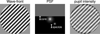 |
Fig. 3 Focal (centre) and pupil-plane (right) images corresponding to a pure spatial frequency wave-front (left) in presence of an amplitude mask. |
3.2 Orthogonal Foucault knife edges with modulation
One straightforward generalisation of the FKE mono-dimensional model presented in Vérinaud (2004) is to consider the information on the WF provided by two distinct orthogonal FKEs with a linear and uniform TT modulation orthogonal to each edge. Under this assumption and following the results presented in Vérinaud (2004), we can rank the modes depending on their Fourier components (u, v) as follows:
G modes (measured like the gradient):

H modes (measured like Hilbert transforms):

where u and v are the spatial frequency coordinates corresponding to X and Y, respectively. rmod is the radius of the modulation circle expressed in units of λ/D, where λ is the wavelength, and D the pupil diameter. For the sake of simplicity, we discarded the H modes with either |u| < rmod/D or |v| < rmod/D because their behaviour is slightly different, but they do not contribute significantly to the error budget.
We considered the definition of the slope-like measurements Sx corresponding to two reciprocal Fourier masks of an FKE as defined in Vérinaud (2004). We added Sy corresponding to an orthogonal FKE. For G modes, the measurements can be written as
![Mathematical equation: $\matrix{ {{S_x}\left[ {{\phi _G}(u,v)} \right] = {{iD} \over {{r_{{\rm{mod }}}}}} \cdot u \cdot {\phi _G}(u,v)} \cr {{S_y}\left[ {{\phi _G}(u,v)} \right] = {{iD} \over {{r_{{\rm{mod }}}}}} \cdot v \cdot {\phi _G}(u,v)} \cr } .$](/articles/aa/full_html/2024/02/aa46660-23/aa46660-23-eq10.png) (6)
(6)
We can trivially note that for any Fourier component with
![Mathematical equation: ${S_x}\left[ {{\phi _G}(u,v)} \right] \ne {S_y}\left[ {{\phi _G}(u,v)} \right],$](/articles/aa/full_html/2024/02/aa46660-23/aa46660-23-eq11.png) (7)
(7)
which means that the information in each component is different. However, for the H modes ϕH(u, v), the situation is different because the measurements can be written as
![Mathematical equation: $\matrix{ {{S_x}\left[ {{\phi _H}(u,v)} \right] = i \cdot {\mathop{\rm sign}\nolimits} (u) \cdot {\phi _H}(u,v)} \cr {{S_y}\left[ {{\phi _H}(u,v)} \right] = i \cdot {\mathop{\rm sign}\nolimits} (v) \cdot {\phi _H}(u,v)} \cr } ,$](/articles/aa/full_html/2024/02/aa46660-23/aa46660-23-eq12.png) (8)
(8)
and we have
![Mathematical equation: ${S_x}\left[ {{\phi _H}(u,v)} \right] = \pm {S_y}\left[ {{\phi _H}(u,v)} \right],$](/articles/aa/full_html/2024/02/aa46660-23/aa46660-23-eq13.png) (9)
(9)
where this time, each component contains the same information because the difference between Sx and Sy is only a sign (and this sign depends on the signal definition alone).
The property of Eq. (9) plays a central in our proposition of a new type of WFS that maximises the sensitivity on the H modes. In the case of an XAO system with a small modulation, H modes are much more frequent than G modes and dominate the overall WF error budget.
 |
Fig. 4 Amplitude masks for each quadrant of the PWS (left) and equivalent masks for the double FKE (right). |
3.3 Foucault knife edge and pyramid
Fauvarque et al. (2016) introduced a 2D model for the FF-WFS that uses the filtering masks for each quadrant as provided in Fig. 4. The corresponding 2D TFs between WF and meta-intensity for a single quadrant of the modulated PWS and for a single modulated FKE are provided in Fig. 5. This figure shows that the TF of a single quadrant of the PWS is characterised by a significant area with a null value (top left and bottom right), which indicates a blind zone in the Fourier space. In comparison, the blind zone of the FKE quadrant is much smaller and is concentrated on frequencies with u = 0. This property as well as the maximum values of the plateaus of the TFs (one-quarter for the PWS and half for the FKE) that is associated with the sensitivity of the sensors are explained in Sect. 5.
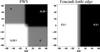 |
Fig. 5 2D transfer functions for a single quadrant of the PWS (left) and for a single FKE (right). A circular TT modulation of 3 λ/D is considered for both cases. The TF general definition is given by Eq. (A.2) and its expression for a single mask is given by Eq. (A.3). |
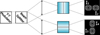 |
Fig. 6 Schematic view of the concept of modulated Bi–O edge sensor based on two refractive roof prisms. |
4 Concept of the bi-orthogonal Foucault knife-edge sensor
Phillion & Baker (2006) studied a two-channel non-modulated sensor with two orthogonal two-sided pyramids, also sometimes called double-roof sensor. This WFS was shown to be a very sensitive direct-phase sensor, but it has a very short dynamic range. For this reason, it was proposed for a second-stage in XAO concept studies such as the Planet Formation Imager (PFI on the TMT; Macintosh 2007 and for the Exo-Planet Imaging Camera and Spectrograph (EPICS at the ELT; Vérinaud et al., 2010). A full double-stage end-to-end simulation of the EPICS AO system can be found in Korkiakoski & Vérinaud (2010).
4.1 Sharp Bi–O edge
The first new concept, named sharp Bi–O edge, is presented in Fig. 6. It consists of a TT beam modulator (e.g. same circular shape and amplitude as the PWS1), followed by a 50/50 beam-splitter. In each channel, the prism is equivalent to two genuine FKEs sharing the same edge. The respective edges in both channels are orthogonal to each other. The sensing is done by recording the intensity in the four re-imaged pupils. The prism of the sharp Bi–O edge has the advantage of being very easy to manufacture, removing the requirement of producing a pointy tip where the sides of the pyramid meet.
The equivalence to FKEs is ensured under the condition that the prisms have a sufficiently large deflection angle to avoid significant leakage between the two diffracted beams. This property is easily met when TT modulation is used. We therefore neglect the leakage term and consider the analysis of the sensors using pure amplitude masks hereafter.
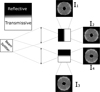 |
Fig. 7 Schematic view of the concept of grey Bi–O edge with reflective or transmissive plates. Black indicates reflective, and white shows transmissive. The gradient-like semi-reflective zone (grey) reaches a 50%/50% ratio in the centre. |
4.2 Grey Bi–O edge
4.2.1 Concept
The second new concept is a variation of the sharp Bi–O edge and is called grey Bi–O edge. It is presented in Fig. 7. In this case, the refractive facets of the prisms are replaced by a 100% reflective or 100% transmissive plates. The TT modulator is removed, and a semi-reflective rectangular zone is present at the location of the edge of the masks that linearly extends from 100% reflective to 100% transmissive. The centre of the mask is exactly 50% reflective and 50% transmissive. This small grey gradient zone is the challenging part of the component because its width is typically of the order of the size of the modulated beam diameter, that is, 10s to 100s of microns in width, and it shall be loss-less.
The grey Bi–O edge concept can also be seen as an evolution of the pupil-plane WF gradient sensor of Horwitz (1994). The grey Bi–O edge masks are Foucault knife-edge masks whose edges have the same properties as the masks derived by Horwitz (1994). Horwitz showed that orthogonal amplitude filters linear in intensity are equivalent to a slope sensor and can be made loss-less and symmetric. An illustration of the resulting mask (horizontal case) is provided in the top left corner of Fig. 7, and a cut of reflectivity or transmission is represented in Fig. 8.
4.2.2 Static modulation
The grey edge plays a similar role as the TT modulation: it reduces the sensitivity of G modes and increases the dynamic range. The geometrical model of Ragazzoni (1996) can be adapted to the grey Bi–O edge. A ray originating from the pupil with some angle (local WF derivative) will be affected by two values, one in each quadrant: the reflectance and the transmittance at the location at which the ray hits the mask. In this way, the effect on the TT mode dynamic range can easily be understood because the signal is expected to be linear over approximately the width of the grey zone. For the other modes, non-linear diffraction effects are more prominent, and more advanced models are needed like in Fauvarque et al. (2016), or an end-to-end model must be used. We expect a qualitatively similar behaviour, in which the dynamic range is affected in an opposite way to the sensitivity and with a similar frequency dependence as suggested by the sensitivity analysis below. A thorough study of the dynamic range as function of modes must definitely be part of a forthcoming study. However, we can reveal some diffraction aspects of the grey edge effect on the sensitivity in the small-phase regime.
Guyon (2005) determined the sensitivity of the PWS for a given Fourier G mode by considering two configurations (see Fig. 5 from Guyon 2005). The first represents signals with maximum fringe contrast (configuration as in Sect. 3.1 when the core interferes with only one speckle), and the second represents signals with a blank pupil (no signal) in a configuration in which the two speckles and the core interfere. The total signal is obtained from the sum of signals weighted by the time passed in each configuration.
The mechanism of static modulation of the grey edge is illustrated in Fig. 9. The figure represents the superposition in transparency of a PSF and the amplitude filter (only the transmitted part is represented, and the grey zone width is enlarged for illustrative purposes). In Sect. 3.1, we mentioned that complex amplitudes of the two speckles have a π phase shift that leads to fringes with opposite sinusoids when each speckle interferes independently with the core. The grey edge modulation mechanism consists of a three-source interference in which the intensity of the two speckles is unbalanced by the amplitude mask. In the case presented in Fig. 9, the signal has the fringes with a phase obtained from the interference with speckle 2, with the coherent addition of the opposite-phase fringed pattern of the interference with speckle 1. This results in a contrast damping that qualitatively explains the reduction of the signal. A quantitative evaluation with this empirical model is complex, especially because of the coherent nature of the sum. Moreover, in the more practical case of a small grey width, the speckle-pinning effect with the core must be taken into account. This can be done by using an end-to-end model that also yields the complete study of the dynamic range.
It is interesting to verify, however, whether the signals for G modes are of a derivative nature, as shown by Horwitz (1994) for a pure gradient mask. We consider the grey edge sensitivity with the help of the C model as in Sect. 3.3. We again use Eq. (A.3), but with rmod = 0 in Eq. (A.4) and with the grey edge amplitude mask equal to the square root of the transmittance (see Fig. 10).
The transfer function (purely imaginary) for one quadrant is represented in Fig. 11. The TF of a sharp Bi–O edge (modulation radius 2λ/D) and of a grey Bi–O edge (grey zone half-width 3λ/D) are provided. The grey width is slightly larger than the TT modulation to include the sensitivity damping due to the circularity of the TT modulation. This figure shows that the grey Bi–O edge measurements for G modes is qualitatively similar to the one provided by the modulated sharp Bi–O edge, that is, to the derivative of the phase.
Finally, as in Sect. 3.3, we can evaluate the level of the plateau of the TFs for H modes: the grey edge sensitivity is  higher than that of the modulated sharp edge. This is also explained in Sect. 5.
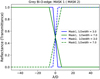 |
Fig. 8 Reflectance (solid line) and transmittance (dashed line) of masks 1 and 2 (modifications of mbio,1 and mbio,2 as defined in the appendix) of the grey Bi–O edge. The curves are represented for two values of the half-width of the grey zone. |
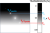 |
Fig. 9 Static modulation mechanism in the case of the grey edge transmitted beam. The image shows the superposition of the square of the amplitude filter with a single Fourier component PSF (G mode). The grey edge width is indicated by two dashed grey lines on the greyscale bar. The blue (speckle 1) and red (speckle 2) expressions indicate the intensity of the speckles after application of the amplitude mask. The signal in the pupil results from the interference of the core with two speckles with an unbalanced intensity. |
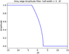 |
Fig. 10 Amplitude filter corresponding to mask 1 of the grey Bi–O edge (cut along X). |
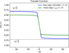 |
Fig. 11 Imaginary part of the transfer function for a single quadrant (cut along X). Comparison between the grey Bi–O edge and the TT-modulated sharp Bi–O edge. |
5 Empirical model for sensitivity and noise propagation
The goal of this section is to predict the performance of the different concepts in terms of sensitivity and noise propagation for G and H modes by observing the signal formation. We used the end-to-end model OOPAO (Heritier et al. 2023)2 and the results of Sect. 3.1 to break down the signal generation along the modulation path. The case of a modulated PWS is considered as our reference and is compared to the sharp and grey Bi–O edge concepts.
The error budget of an AO system giving the residual phase variance  can be written as the sum of the fitting, temporal, aliasing, and noise propagation error variances,
 (10)
(10)
We assumed that the WFS detector is only affected by photon noise, and so is the noise propagation,
 (11)
(11)
The derivation of σph for an FF-WFS has been given in Fauvarque et al. (2016). We write this term under the assumption of a uniform pupil illumination and conservation of incident flux in the geometrical pupils. These suppositions are met in the small-phase regime and when the diffraction by the edges of the masks is neglected. σph can then be written as
 (12)
(12)
where the sensitivity χ(ϕ) with respect to the phase ϕ is defined in Eq. (1). In the case of multiple components (as in the case of slope measurements), the sensitivity is the quadratic sum of the sensitivity for each component,
 (13)
(13)
 is the measurement variance due to photon noise alone. In the following, we use these formulas to derive a theoretical performance comparison when ϕ is either a G or an H mode.
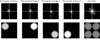 |
Fig. 12 Illustration of the signal creation for the PWS during a modulation cycle. Top: view of the focal plane of the PWS during the different phases of the modulation cycle. Bottom: Corresponding signal created on the detector. The corresponding integrated modulation path and signal are displayed in the right part of the figure. |
5.1 Application to the PWS
The PWS (see Fig. 1) produces four pupil images on the WPS detector. The sub-aperture resolution is then given by the WFS detector pixels that sample the pupil. For each of the four pupils, the image intensities are given by Ii(x, y), with i being the pupil index, and (x, y) being the pixel coordinates. With N the incident flux per sub-aperture (four pixels) and per frame, the slope-like measurement definition Sx and Sy with global normalisation (Vérinaud 2004) is defined as
 (14)
(14)
 (15)
(15)
In these equations, N is a fixed normalisation factor, and Ii(x, y) is the variable signal. The variance of the signal in each pixel is (Poisson’s statistics)
 (16)
(16)
From Eqs. (14) and (15), we computed the measurement noise variance  ,
,
 (17)
(17)
To derive the sensitivity term χ, it is necessary to carry out a more complex analysis: ϕ must be distinguished between G and H modes, and the impact of the TT modulation path must be included. We introduce the concept of modulation duty-cycle per quadrant DCmod to quantify the fraction of the time during which the signal is created on a quadrant along one full modulation cycle.
For G modes, which produce intensity perturbations close to the core of the PSF, the TT modulation dispatches the light in the four quadrants so that each quadrant contributes to the signal. In these conditions, G modes are well described by a geometric model like in Ragazzoni (1996), where the measurement is a quad-cell-like (denoted QC) derivative and is given by Eq. (6). Let  denote the PWS sensitivity to the G modes. For G modes, the sensitivity term explicitly depends on the variables (u, v). However, for the sake of simplicity, we hide these variables. Equation (12) can then be written for the G modes as
 (18)
(18)
For H modes, the situation is different: The signal is created only when the interfering core and speckle are located in the same quadrant. We know from Eq. (5) that the corresponding sensitivity is equal to unity (χCS = 1).
Figure 12 gives the details for the PWS and illustrates when the signal is created for the four one-quarter of the frames in one modulation cycle. Because of the separation between speckle and core and the shape of the masks, the signal is created only during one-quarter of the frames for each quadrant, and two quadrants receive no signal. The duty cycle  per quadrant therefore is 25%.
By evaluating Eqs. (14) and (15), we obtain
 (19)
(19)
where the factor of 2 arises from the subtraction of the two fringed pupils that are π-shifted one from the other. In the example for  , the signal comes from the subtraction of pupil 1 from pupil 3. Then we have
 (20)
(20)
Equation (12) can then be written for the H modes as
 (21)
(21)
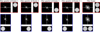 |
Fig. 13 Signal created for each quarter of a full modulation cycle for the sharp Bi–O edge. The red frames correspond to the first channel (split horizontally), and the blue frames show the second channel (split vertically). |
5.2 Application to the sharp Bi–O edge
For the Bi–O edge (sharp and grey), we use the subscript ‘bio’ whenever an assertion is applicable to both the sharp (‘sha’) and the grey (‘gre’) concept. We define the measurements in X and Y as
 (22)
(22)
 (23)
(23)
This definition takes into account that the flux is split into two channels, each receiving half of the flux. The corresponding measurements variance due to photon noise is
 (24)
(24)
We can note that the Bi–O edge measurement variance  is twice that of the PWS given by Eq. (17).
For G modes, the geometrical model used in Ragazzoni (1996) can be directly applied to the sharp Bi–O edge3 and gives the same result:
 (25)
(25)
The noise propagated on G modes for the sharp Bi–O edge is
 (26)
(26)
The G mode noise propagation of the sharp Bi–O edge is therefore twice higher than for the PWS. This behaviour was intuitively expected because X- and Y-slopes are only derived using half of the total flux because of the beam splitting. For the PWS, the slopes are instead calculated using all available photons.
For the H modes, the details of the modulation cycle for a sharp Bi–O edge are provided in Fig. 13 and show that in contrast to the PWS, all quadrants provide a signal half of the time  .
.
We can then compute the associated sensitivity of the sharp Bi–O edge as
 (27)
(27)
The complete sensitivity term is
 (28)
(28)
Eq. (12) can then be written for the H modes as
 (29)
(29)
The H mode noise propagation of the sharp Bi–O edge is therefore twice lower than for the PWS. This behaviour can also be understood intuitively: The Bi–O edge generates signal throughout a modulation cycle, while the PWS is blind to a particular H mode half of the time (e.g. during one-quarter of frames 2 and 4 in Fig. 12).
5.3 Application to the grey Bi–O edge
We assumed that the width of the grey zone is π/2 times larger than the diameter of the circular modulation in order to account for the difference in sensitivity between the linear and circular shape. Under these assumptions, and because the measurements definition is the same as in Eqs. (22) and (23), we have for G modes
 (30)
(30)
 (31)
(31)
The grey Bi–O edge signal formation for H modes is represented in Fig. 14. As for the sharp Bi–O edge, there is no blind zone. The efficiency is 100% of the duty cycle. However, because the flux in the core is split equally between reflected and transmitted beams, the sensitivity χl/2CS corresponding to the interference between half of the core and a speckle is reduced by a factor  in accordance with Eq. (2), and we have
 (32)
(32)
We can then compute the sensitivity of the grey Bi-O edge as
![Mathematical equation: $\matrix{ {{\rm{T}}{{\rm{F}}_{y,pyr}} = 2i[{m_{pyr,3}}\left( {{m_{pyr,2}}\omega } \right) - {m_{pyr,2}}\left( {{m_{pyr,3}}\omega } \right)} \hfill \cr {\,\,\,\,\,\,\,\,\,\,\,\,\,\,\,\,\,\, + {m_{pyr,1}}\left( {{m_{pyr,4}}\omega } \right) - {m_{pyr,4}}\left( {{m_{pyr,1}}\omega } \right)]} \hfill \cr } $](/articles/aa/full_html/2024/02/aa46660-23/aa46660-23-eq47.png) (33)
(33)
The complete sensitivity term is
 (34)
(34)
Equation (12) can then be written for the H modes as
 (35)
(35)
The H mode noise propagation of the grey Bi–O edge is therefore twice lower than for the sharp Bi–O edge and four times lower than for the PWS. This represents a significant advantage for AO, which frequently struggles with the limited number of photons provided by the AO guide star. Intuitively, the grey Bi–O edge makes better use of the photons because H modes produce signal in all quadrants all the time instead of only half of the time for the sharp Bi–O edge with modulation. Even considering the fringe contrast loss of  (Eq. (32)), this leads to a net gain of a factor of 2 in efficiency to the use of photons. This is analogous to the improved sensitivity of the non-modulated PWS over the modulated one even for very little modulation (Guyon 2005).
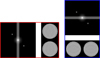 |
Fig. 14 Signal creation for the grey Bi–O edge. The grey stripe represents the zone with gradient-shape reflectivity or transmissivity. |
5.4 Summary
We summarise in Table l all the findings of Sect. 5. The result of Eq. (12) represents the behaviour of the noise propagation for the different concepts for G and H modes.
For G modes, a PWS presents a twice lower noise propagation (1/N) than the Bi–O edge concepts (2/N) because the split of light in the latter reduces the number of photons for measuring each component of the derivative by a factor of 2.
For H modes, the sharp Bi–O edge presents a twice lower noise propagation (1/N) than the PWS (2/N). One way to understand this is that the Hilbert transform carries all the information and hence does not suffer from the split of light (in our readnoise-free hypothesis). Moreover, the Fourier masks of the PWS are such that two quadrants are blind to a given H mode. The grey Bi–O edge gains another factor of 2 (1/(2N)) with respect to the sharp Bi–O edge (1/N) because of the static nature of the modulation. Section 6 analyses in detail how the noise propagation is distributed on the G and H modes and how this determines the overall noise propagation.
6 Analysis of the Bi–O edge performance gains
6.1 Modal noise propagation
The empirical model of Sect. 5 makes a rigid distinction between G and H modes without considering how many modes of each type the system contains and neglecting the fact that modes with a spatial frequency around the modulation circle have mixed properties. In practice, small modulation angles (few λ/D) are used in PWS systems, and the number of DoF is limited for various reasons and can be very diverse in the AO systems. We perform an improved analysis in this section in order to derive the trend of performance gains as a function of controlled modes.
We performed the analysis for systems with realistic configurations and number of DoF and for a typical modulation radius of 2 λ/D (half-width=3λ/D for the grey Bi–O edge). Our reference case is the ELT Single Conjugate Adaptive Optics (SCAO) first-light system, which is the Phasing and Diagnostic Station (PDS) PWS-based AO system with 3000 controlled modes (Bonnet et al. 20l8). This number of modes is conservative, but is found to match the analytical model well based on a least-squares reconstruction developed in the appendix. We develop in Appendix A the formalism of the C model of Fauvarque et al. (20l9) of the PWS and Bi–O edge variants and derive the modal properties of noise propagation.
An example of the modal noise propagation curves obtained using this formalism (Eqs. (A.16) and (A.17)) is shown in Fig. 15 for the three concepts and for the ELT SCAO configuration. 3000 modes were corrected and the sensing was made in K band to stay in the linear regime that is the assumption in this paper. The figure shows that the noise propagation of the high-order H modes follows the expected tendency, but the relative gains are somewhat reduced (factor ≈1.6 and ≈3 gain by the grey BiO edge over the sharp Bi–O edge and the PWS, respectively, instead of factors of 2 and 4). Figure 15 also shows that even though the noise propagation on G modes or low orders is very strong, the number of H modes is largely dominant for the chosen modulation amplitude. Figure 16 shows a close-up on the low-order or G modes.
The overall performance is given by the total noise propagation error variance Vwfs and is obtained by integrating Eq. (A.11),
 (36)
(36)
where the theoretical integration area A is
 (37)
(37)
In order to estimate the overall sensitivity gain with respect to the PWS, we define in Eq. (38) the gain ratio Gwfs/pyr(ikl), where wfs is the sharp Bi–O edge or the grey Bi–O edge. From Sect. 5, we know that this factor is comprised between half (in the case of a very low-order system, only G modes matter) and four (for a grey Bi–O edge system in which very high orders dominate),
 (38)
(38)
The gain in function of the number of modes that are corrected can be computed by adapting the integration area in Eq. (36) because the cut-off frequency fc = 1/(2d) is never really attained in a real system. For the SCAO ELT configuration, we simulated the PDS case with 3000 modes, which corresponds to a cut-off frequency of 0.7 fc. We used this value as the upper limit of the integration, and for each value of d, the number of modes was adjusted accordingly. We also used a conservative approach to include the low-order noise propagation: some preliminary work that goes beyond the scope of this paper suggests that the C model limitations related to the integration over a finite pupil (Fauvarque et al. 2019) lead to an underestimation of the noise propagated on low orders. We found out that extending the integration down to fmin = 1/(4D) gives an improved estimation of the low-order contribution that is sufficient to obtain the right trends. The corrected overall noise propagation variance V′ was obtained by integrating the circular averaged noise propagation for different values of d in order to predict the gain for different numbers of corrected modes,
 (39)
(39)
The result is represented in Fig. 17 and describes the gain in function of corrected modes. The two additional points were computed from the noise propagation obtained using calibration data of the end-to-end model for the ELT SCAO system with 3000 controlled modes.
For the sharp and grey Bi–O edge concepts, the low-order system limit shows the expected loss of a factor of 2 in photon efficiency. For very high-order systems (105 modes), the gain for the grey Bi–O edge reaches a factor of 3 (1.2 mag), and the sharp Bi–O edge is limited to 1.6 (0.6 mag). The validation through end-to-end closed-loop simulations is presented in the next section.
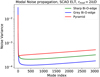 |
Fig. 15 Noise propagation per mode for SCAO/ELT configuration (3000 modes, sensing in K band) for a 2λ/D modulation radius. |
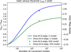 |
Fig. 17 Gain with respect to the PWS as a function of corrected modes for the SCAO/ELT configuration (3000 modes, a 2λ/D modulation radius, sharp-Bi–O edge, and grey Bi–O edge). |
6.2 End-to-end simulations
We developed a diffractive model of the two Bi–O edge concepts and added it to the OOPAO package. We simulated pure amplitude masks for both the PWS and the Bi–O edge. Our reference configuration for the simulation was that of the ELT SCAO with 3000 modes.
The main parameters used in the simulation can be found in Table 2. We used the SCAO ELT K-band case in which the sensors are used close to their linear regime, which is the assumption of this paper. Moreover, we assumed null read-out noise such that the performance degradation at low flux is dominated by photon noise error propagation. The performance in terms of SR and as a function of the flux is displayed in Fig. 18.
These results confirm the gains obtained with the analytical model. For instance, for a relative drop in SR of 25%, that is, for SR = 64.5%, 2.7 photons are required for the PWS, 1.75 for the sharp Bi–O edge, and 1.11 for the grey Bi–O edge. This gives a gain versus the PWS of 1.54 for the sharp and 2.43 for the grey Bi–O edge. In Fig. 17, the gains predicted from the C model are 1.41 and 2.33, respectively, which is slightly pessimistic, but very close to the end-to-end results.
As a side note, we mention that for simplicity, we limited the content of the paper to one modulation angle (rmod = 2λ/D and grey edge half-width = 3λ/D) that we believe is realistic for XAO with reasonably low residuals. We concentrated the effort on this case to obtain consistent results between analytical and end-to- end simulations. We initiated some work to consider different modulation angles that showed that some aspects of the theoretical model must be adjusted. From these preliminary results, we observe that the behaviour for a high number of corrected modes is merely independent of the modulation angle. We estimate that the gain for rmod = 3λ/D would be about 5% lower than for rmod = 2λ/D for more than 104 corrected modes. The strongest impact is on the tipping point, where the Bi–O edge gain is larger than one, that is, when the G mode noise propagation becomes small in the error budget. Figure 17 shows that more than 400 modes are needed to see a gain with the sharp Bi–O edge with rmod = 2λ/D. We estimate this number to be close to 100 modes for rmod = 1λ/D and 800 modes for rmod = 3λ/D. Future work will refine this analysis and also include the grey Bi–O edge. We also mention that the case rmod = 0 was discarded because it cannot be treated well with the assumptions of this paper (uniformity and flux conservation in the pupil).
It is also remarkable that for a flux of only 0.5 photons per sub-aperture and frame, the performance of the Bi–O edge concepts is still decent, with a drop of only 50% in SR for the grey Bi–O edge, while the PWS is not able to close the loop. These analyses will certainly need to be improved by taking into account an optimisation of the control with respect to flux, but they definitely validate the overall analysis of the Bi–O edge concepts sensitivity advantage. Future analysis will also consider detector read-out-noise in the simulations. The factor of 2 of noise variance between the PWS and Bi–O edge will remain when considering additional read-out-noise. This can be shown by rewriting Eqs. (17) and (24), where ron is the readout-noise in photo-electron per pixel (see Eqs. (40) and (41)). However, because the read-out-noise term has a quadratic dependence on the number of photons, the stellar magnitude gain in Fig. 17 would be reduced depending on read-out-noise, but also on the stellar flux itself. Modern avalanche-photo-diode-based cameras can have read-out noise as low as 0.6 electrons (e.g. Feautrier & Gach 2022). This will clearly strongly affect the SR curves of Fig. 18 at very low flux. However, in HCI, the limitation due to stellar flux will most probably first affect the halo of residuals (the contrast) before a noticeable drop of the SR occurs. With a refined criterion relevant for HCI, the corresponding natural guide star (NGS) limiting magnitudes would occur at higher fluxes, such that the additional read-out-noise term would be not far from one. For instance, with ron = 0.6 and for N = 10 photons, the corrective term is 1.114, while it is 2.44 for N = 1,
 (40)
(40)
 (41)
(41)
Numerical simulation parameters.
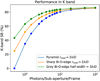 |
Fig. 18 SR as a function of flux for the SCAO/ELT configuration (3000 modes, 2λ/D modulation radius). |
7 Conclusion
We revisited the concept of dual-channel two-sided PWS by realising that this concept is the implementation of two orthogonal FKEs. In order to keep the dynamic range of the PWS, we introduced the TT modulation to the concept, denoted as the sharp Bi–O edge concept. By designing a reflective version, we realised that the modulation functionality can be achieved by implementing a reflective or transmissive central stripe with gradually changing reflectivity and transmission. We dubbed this concept the grey Bi–O edge.
We used an empirical model to evaluate the efficiency of the FKE masks as used by the different concepts. Splitting the light between two channels penalises the low orders (or G modes), such that both Bi–O edge flavours would need twice more photons than a PWS to reach the same noise propagation level in a low-order system.
However, in a high-order system, the amount of noise propagated on low orders or G modes is relatively small compared to the H modes. These high-order modes have the remarkable property that their measurement from the FKE in both channels carries the same information. This redundancy is responsible for the fact that the sensitivity is not impaired by the separation in flux and covers the full Fourier plane. This is not the case for the PWS, as shown by the TFs of the amplitude masks in Fig. 5 and the modulated signal decomposition in Fig.12: each of the four PWS pupils is blind to one-half of the Fourier plane. This lack of the PWS also explains why the sharp Bi–O edge in the empirical model shows a factor of 2 higher photon efficiency for H modes. Even better, because the grey Bi–O edge has a 100% modulation duty cycle, it gains another factor of 2 over the sharp Bi–O edge, which only has a 50% duty cycle.
The empirical model of Sect. 5 is very simplified on purpose. For a study with much greater generality than ours, we suggest to consider Chambouleyron et al. (2023). In this paper, the notion of photon noise sensitivity has been updated and shown to have an upper limit at 2, twice more than what was thought before (e.g. see Guyon 2005). Figure 1 of Chambouleyron et al. (2023) shows how the Zernike sensor sensitivity (for H modes) can be increased until it is very close to 2 at the expense of a major loss of sensitivity for G modes. Table 1 of the present paper can directly be used to determine this same sensitivity by identifying the coefficient in front of 1/N as the inverse of the photon sensitivity squared. This gives for the photon sensitivity (to H modes) a value of  for the modulated PWS (compatible with Chambouleyron et al. 2023), 1 for the modulated sharp Bi–O edge (close to the classical Zernike: 1.25), and
  for the grey Bi–O edge, which is remarkable provided that the grey Bi–O edge is a sensor conceived to have sufficient dynamic range to be used in a stand-alone AO system.
In Sect. 6.1, we improved the accuracy of the results obtained from the empirical model through a model that was based on the work by Fauvarque et al. (2019). The C model permitted us to show how the number of controlled modes come into play. Finally, results from an end-to-end model (Sect. 6.2) have confirmed the gain expected for the ELT SCAO configuration in the linear regime.
There are different directions for future works on an analytical and simulation point of view and regarding practical implementations. The first important point is to develop the formalism and simulations for systems with high residuals in order to take optical gain into account (e.g. Deo et al. 2021; Chambouleyron et al. 2020) and determine whether the advantages of the Bi–O edge are conserved when the small-phase regime is not met.
We will also study the effect of WF discontinuities in giant segmented-mirror telescopes (GSMTs) (e.g. Bertrou-Cantou et al. 2022). Preliminary simulations indicate that the Bi–O edge and the PWS behave similarly in presence of phase discontinuities. For example, both can measure petal errors, which are smaller than the sensing wavelength, but suffer from the phasewrapping problem for large amplitudes (Pourré et al. 2022). We also expect the impact of segment co-phasing residuals to be similar to the PWS.
From a fundamental point of view, the property expressed in Eq. (9) has an even more profound consequence than the one we identified on the sensitivity. The four times redundant H mode measurements in each quadrant can take advantage of the implementation of super-resolution (Oberti et al. 2022). This will significantly improve the accuracy of very high orders by rejecting aliasing. Beyond the possibility to even control more modes classically allowed for a given resolution, this enrichment of the signal could be very beneficial for controlling non-linearity with advanced model-based WF reconstruction schemes (e.g. Hutterer et al. 2023) as well as with machine-learning techniques (e.g. Nousiainen et al. 2022), and it may help to solve some ELT-related issues such as the differential pistons issues (Bertrou-Cantou et al. 2022). Super-resolution will be the topic of a forthcoming paper.
Practically speaking, the sharp Bi–O edge can be seen as a mild evolution of the PWS concept with certainly an advantage for the manufacturing of accurate single-edge prisms. Its implementation would require only minimal developments. For XAO on an 8m class telescope (e.g. with 1000 correction modes), the sharp Bi–O edge would bring a gain of about 0.2 mag with respect to the PWS and a gain of about 0.5 mag for XAO on an ELT.
The advantage of the grey Bi–O edge is very significant because the gain changes from 0.7 mag on an 8m class telescope to 1.1 mag on the ELT for the current PCS baseline (≈104 modes), which may have a significant impact on the number of available scientific targets: In this case, to reach a similar AO performance as with a PWS, the Bi–O edge can use 2.7 times fewer photons. Hence, it can use guide stars that are up to  times farther away, which corresponds to an observable volume that is more than four times larger (we note that for 104 corrected modes, the sharp Bi–O edge presents a gain of 1.6, corresponding to an observable volume about twice larger than the PWS). A forthcoming work will study the real impact on science in detail by evaluating the S/N of coronagraphic images assisted by Bi–O edge-based AO systems.
In addition to the high sensitivity, the absence of a TT modulation device presents an important advantage of the grey Bi–O edge. In addition to the simplification of the design, the grey Bi–O edge is not limited by the mechanical dynamics of a fast steering mirror and is limited only by the WFS camera and real-time computer speeds.
However, the complexity will be manufacturing a (preferably) loss-less grey-scaled edge with a typical width of 100 μm. One of the class of techniques we have thought about so far is the beam splitting by a division of amplitude. This can be done, for instance, by depositions of metal coatings of different depth, by using dielectric plates, or by using rotators and polariser beamsplitters (e.g. Gendron et al. 2010; Haffert 2016; Snik et al. 2012). To handle the variability of the mask and make advantageous use of micro-lithography techniques, we envision defining a discretisation of the amplitude. While waiting for detailed simulations, we evaluate the need for a minimum value of two resolution elements per λ/D (e.g. 12 steps for a grey half-width of 3λ/D). This discretisation will also help with adjustments during the process and deal with issues such as amplitude-dependent phase shifts, which are likely to occur. One technique among these solutions, patterned liquid crystal, has already been tested and even demonstrated on sky for the validation of a generalised optical differential sensor (Haffert et al. 2018). Even though the manufactured mask is significantly less demanding in terms of amplitude variation than a grey FKE, this achievement is really remarkable and contributes to favouring polarisation techniques.
Splitting the beam by division of wavefront is certainly the cheapest and least risky solution. We can use a typical technique employed in coronagraphy by using micro-lithography with reflective microdots (Martinez et al. 2009). Very high resolution (micrometers) can be obtained, such that there is probably no need for a discretisation like the one mentioned for the division of amplitude. The division between reflected and transmitted beam can be made very clean and will not introduce any amplitude-dependent phase shift. However, the main drawback is that because the microdots must encode the desired focal- plane amplitude (and not the intensity), the amount of reflected light and transmitted light is asymmetric by nature and leads to diffraction losses. Still, the microdot pattern could be optimised for the transmitted beam alone (or for the reflected beam), which contains all the WF phase information. This concept would be simpler to implement opto-mechanically and may still be competitive in terms of sensitivity with the sharp Bi–O edge, but with the advantage of the static modulation.
The overall opto-mechanical concepts for integrating two orthogonal FKEs need to be explored, especially to reach sufficiently compact designs with minimum non-common path aberrations (NCPA). The number of detectors is also an important topic. The sharp Bi–O edge has two channels, so that two detectors is a logical solution. However, a smart design gathering all pupils on one detector should be possible without increasing NCPA. Because the WF is encoded into an intensity signal at the level of the masks, only optics before the masks contribute significantly to the NCPA. The grey Bi–O edge has four channels, so that four detectors is one potential solution. This may even be an advantage for very high-order XAO and could allow a fine adjustment of the pixel grid alignment for implementing super-resolution. Here also, smart designs may reduce the number of required detectors. For instance, the polarisation technique could be based on transmissive optics (Wollaston prisms or patterned liquid crystal), which will allow more compact designs. To conclude, the bi-orthogonal Foucault knife-edge sensor with its outstanding capabilities in terms of sensitivity and resolution is a timely new WFS candidate for the coming challenges in the field of HCI especially on GSMTs.
Appendix A Noise propagation with the C model
Definitions
In this section, we present the mathematical definitions used for the C model. The direct space variables are (x, y). The corresponding Fourier space variables are (u, v) and  represents the Fourier transform. The sampling size of the detector pixel projected on the telescope input pupil is d. The WFS focal-plane amplitude filter is mwfs (u, v). The TF for quadrant k is TFk(u, v). The WF phase at location x, y is ϕ(x, y). The PWS is described by four binary masks (see Carbillet et al. 2005). We used the same definition and enumeration as in Fauvarque et al. (2019), and for the Bi–O edge, we extended it to the four FKE masks represented in Fig. 4. We express the masks in the Fourier space,
mpyr,1 := 1 for u < 0 and v > 0
mpyr,2 := 1 for u > 0 and v > 0
mpyr,3 := 1 for u < 0 and v < 0
mpyr,4 := 1 for u > 0 and v < 0.
For the sharp Bi–O edge, the mask definition is
mbio,1 := 1 for u < 0
mbio,2 := 1 for u > 0
mbio,3 := 1 for v < 0
mbio,4 := 1 for v > 0.
By analogy with the PWS, we call the pupil image resulting from the diffraction by a mask a ’quadrant’.
Sensitivity and noise propagation
In this section, we derive the equivalent of Eq. 12. With the C model (Fauvarque et al. 2019), we can describe the sensitivity for any spatial frequencies. We define the noise propagation density in Fourier space,
 (A.1)
(A.1)
where Nph is the incident flux in the input pupil (photons/m2 / frame) and  defines the noise propagation function.
Transfer function
The noise propagation function βR,wfs is obtained from the TFs of the sensors. We call the meta-intensities in Fourier space with infinite spatial resolution  . The TF is defined as
 (A.2)
(A.2)
The TF for a generalised phase and amplitude mask mwfs,k(u, v) is given by (Fauvarque et al. 2019)
 (A.3)
(A.3)
where .* denotes the complex conjugate and the circular modulation function ω(u, v) including diffraction is equal to
 (A.4)
(A.4)
where  . We used the pure amplitude masks representation and the slope-like measurements definition (Eqs. 14 and 15 for the PWS, and Eqs. 22 and 23 for the Bi–O edge) and applied the C model to obtain the TFs. The TF corresponding to the PWS slope-like definition is (correcting a sign in equation B13 of Fauvarque et al. 2019)
 (A.5)
(A.5)
 (A.6)
(A.6)
where ⊛ is the symbol for convolution. A similar calculation gives the TF of the measurements for the Bi–O edge,
 (A.7)
(A.7)
 (A.8)
(A.8)
Noise propagation in Fourier space
The sensitivity of a sensor depends on the resolution or pixel size d (measured in the entrance pupil reference). The meta-intensity Mx is the pixel-filtered version (same for y),
 (A.9)
(A.9)
where the measure and average function  is given by (same for y)
 (A.10)
Following a similar development as in Jolissaint et al. (2006), we obtain the propagated noise,
 (A.11)
We define the noise propagation coefficients as
 (A.12)
We define
 (A.13)
γmI is the result of the calculation of the theoretical variance of the meta-intensities σN,PYR and σN,BIO (see Eqs. (17) and (24)). Finally, we can write the function  as
as
 (A.14)
Modal noise propagation
We derive an approximate correspondence between spatial frequency and mode index. With  the modulus of the spatial frequency, we define an index called ikl(fr), that is, the index of each mode (e.g. Karhunen Loeve (KL) modes). The corrected lowest-order modes are tip and tilt, and they correspond to the spatial frequency
  . We write the effective order of the modes,
 (A.15)
We assume that Noll’s indexing convention holds (Noll 1976) and write the KL index to frequency fr correspondence (including all azimuthal orders until fr),
 (A.16)
The modal noise propagation coefficients from the C model is obtained by circularly averaging Eq. A.12 and normalising by the telescope surface to obtain the noise variance per mode,
 (A.17)
where Ωtel is the surface of the telescope in m2.
References
- Agapito, G., Pinna, E., Esposito, S., et al. 2023, A&A, 677, A168 [NASA ADS] [CrossRef] [EDP Sciences] [Google Scholar]
- Bertram, T., Absil, O., Bizenberger, P., et al. 2018, SPIE Conf. Ser., 10703, 1070314 [NASA ADS] [Google Scholar]
- Bertrou-Cantou, A., Gendron, E., Rousset, G., et al. 2022, A&A, 658, A49 [NASA ADS] [CrossRef] [EDP Sciences] [Google Scholar]
- Beuzit, J. L., Demailly, L., Gendron, E., et al. 1997, Exp. Astron., 7, 285 [Google Scholar]
- Beuzit, J. L., Vigan, A., Mouillet, D., et al. 2019, A&A, 631, A155 [NASA ADS] [CrossRef] [EDP Sciences] [Google Scholar]
- Bond, C. Z., Cetre, S., Lilley, S., et al. 2020, J. Astron. Telescopes Instrum. Syst., 6, 039003 [NASA ADS] [Google Scholar]
- Bonnet, H., Biancat-Marchet, F., Dimmler, M., et al. 2018, SPIE Conf. Ser., 10703, 1070310 [NASA ADS] [Google Scholar]
- Carbillet, M., Vérinaud, C., Femenía, B., Riccardi, A., & Fini, L. 2005, MNRAS, 356, 1263 [NASA ADS] [CrossRef] [Google Scholar]
- Chambouleyron, V., Fauvarque, O., Janin-Potiron, P., et al. 2020, A&A, 644, A6 [EDP Sciences] [Google Scholar]
- Chambouleyron, V., Fauvarque, O., Plantet, C., et al. 2023, A&A, 670, A153 [NASA ADS] [CrossRef] [EDP Sciences] [Google Scholar]
- Clénet, Y., Buey, T., Gendron, E., et al. 2018, SPIE Conf. Ser., 10703, 1070313 [Google Scholar]
- Correia, C. M., Fauvarque, O., Bond, C. Z., et al. 2020, MNRAS, 495, 4380 [NASA ADS] [CrossRef] [Google Scholar]
- Costa, J. B. 2005, Appl. Opt., 44, 60 [Google Scholar]
- Crane, J., Herriot, G., Andersen, D., et al. 2018, SPIE Conf. Ser., 10703, 107033V [NASA ADS] [Google Scholar]
- Deo, V., Gendron, É., Vidal, F., et al. 2021, A&A, 650, A41 [NASA ADS] [CrossRef] [EDP Sciences] [Google Scholar]
- Dressing, C. D., & Charbonneau, D. 2013, ApJ, 767, 95 [Google Scholar]
- Esposito, S., & Riccardi, A. 2001, A&A, 369, L9 [NASA ADS] [CrossRef] [EDP Sciences] [Google Scholar]
- Esposito, S., Mesa, D., Skemer, A., et al. 2013, A&A, 549, A52 [NASA ADS] [CrossRef] [EDP Sciences] [Google Scholar]
- Fauvarque, O., Neichel, B., Fusco, T., Sauvage, J.-F., & Girault, O. 2016, Optica, 3, 1440 [Google Scholar]
- Fauvarque, O., Janin-Potiron, P., Correia, C., et al. 2019, J. Opt. Soc. Am. A, 36, 1241 [Google Scholar]
- Feautrier, P., & Gach, J.-L. 2022, SPIE Conf. Ser., 12183, 121832E [Google Scholar]
- Foucault, L. 1859, Ann. Observ. Paris, 5, 197 [NASA ADS] [Google Scholar]
- Fusco, T., Sauvage, J. F., Petit, C., et al. 2014, SPIE Conf. Ser., 9148, 91481U [NASA ADS] [Google Scholar]
- Gendron, E., Brangier, M., Chenegros, G., et al. 2010, in Adaptative Optics for Extremely Large Telescopes, 05003 [CrossRef] [Google Scholar]
- Give’on, A., Kern, B., Shaklan, S., Moody, D. C., & Pueyo, L. 2007, SPIE Conf. Ser., 6691 66910A [Google Scholar]
- Guyon, O. 2005, ApJ, 629, 592 [NASA ADS] [CrossRef] [Google Scholar]
- Haffert, S. Y. 2016, Opt. Express, 24, 18986 [NASA ADS] [CrossRef] [Google Scholar]
- Haffert, S. Y., Wilby, M. J., Keller, C. U., et al. 2018, SPIE Conf. Ser., 10703, 1070323 [Google Scholar]
- Hénault, F., Spang, A., Feng, Y., & Schreiber, L. 2020, Eng. Res. Express, 2, 015042 [CrossRef] [Google Scholar]
- Heritier, C. T., Verinaud, C., & Correia, C. M. 2023, OOPAO: Object Oriented Python Adaptive Optics, Adaptive Optics for Extremely Large Telescopes, 7th ed. [Google Scholar]
- Hoeijmakers, H. J., Schwarz, H., Snellen, I. A. G., et al. 2018, A&A, 617, A144 [NASA ADS] [CrossRef] [EDP Sciences] [Google Scholar]
- Horwitz, B. A. 1994, SPIE Conf. Ser., 2201, 496 [NASA ADS] [Google Scholar]
- Hutterer, V., Neubauer, A., & Shatokhina, J. 2023, Inverse Probl., 39, 035007 [NASA ADS] [CrossRef] [Google Scholar]
- Jolissaint, L., Véran, J.-P., & Conan, R. 2006, J. Opt. Soc. Am. A, 23, 382 [CrossRef] [PubMed] [Google Scholar]
- Jovanovic, N., Martinache, F., Guyon, O., et al. 2015, PASP, 127, 890 [NASA ADS] [CrossRef] [Google Scholar]
- Kasper, M., Cerpa Urra, N., Pathak, P., et al. 2021, The Messenger, 182, 38 [Google Scholar]
- Keppler, M., Benisty, M., Müller, A., et al. 2018, A&A, 617, A44 [NASA ADS] [CrossRef] [EDP Sciences] [Google Scholar]
- Konopacky, Q. M., Barman, T. S., Macintosh, B. A., & Marois, C. 2013, Science, 339, 1398 [Google Scholar]
- Korkiakoski, V., & Verinaud, C. 2010, SPIE Conf. Ser., 7736, 773643 [NASA ADS] [Google Scholar]
- Lagrange, A. M., Bonnefoy, M., Chauvin, G., et al. 2010, Science, 329, 57 [Google Scholar]
- Macintosh, B. 2007, in Advanced Maui Optical and Space Surveillance Technologies Conference, ed. S. Ryan, E62 [Google Scholar]
- Macintosh, B., Graham, J. R., Barman, T., et al. 2015, Science, 350, 64 [Google Scholar]
- Macintosh, B., Chilcote, J. K., Bailey, V. P., et al. 2018, SPIE Conf. Ser., 10703, 107030K [Google Scholar]
- Malbet, F., Yu, J. W., & Shao, M. 1995, PASP, 107, 386 [NASA ADS] [CrossRef] [Google Scholar]
- Males, J. R., Close, L. M., Miller, K., et al. 2018, SPIE Conf. Ser., 10703, 1070309 [NASA ADS] [Google Scholar]
- Marois, C., Lafrenière, D., Doyon, R., Macintosh, B., & Nadeau, D. 2006, ApJ, 641, 556 [Google Scholar]
- Martinez, P., Dorrer, C., Aller Carpentier, E., et al. 2009, A&A, 495, 363 [NASA ADS] [CrossRef] [EDP Sciences] [Google Scholar]
- Mawet, D., Pueyo, L., Lawson, P., et al. 2012, SPIE Conf. Ser., 8442, 844204 [NASA ADS] [Google Scholar]
- Mawet, D., Bond, C. Z., Delorme, J. R., et al. 2018, SPIE Conf. Ser., 10703, 1070306 [NASA ADS] [Google Scholar]
- Noll, R. J. 1976, J. Opt. Soc. Am., 66, 207 [Google Scholar]
- Nousiainen, J., Rajani, C., Kasper, M., et al. 2022, A&A, 664, A71 [NASA ADS] [CrossRef] [EDP Sciences] [Google Scholar]
- Oberti, S., Correia, C., Fusco, T., Neichel, B., & Guiraud, P. 2022, A&A, 667, A48 [NASA ADS] [CrossRef] [EDP Sciences] [Google Scholar]
- Oti, J. E., Canales, V. F., & Cagigal, M. P. 2005, MNRAS, 360, 1448 [NASA ADS] [CrossRef] [Google Scholar]
- Phillion, D. W., & Baker, K. 2006, SPIE Conf. Ser., 6272, 627228 [NASA ADS] [Google Scholar]
- Pourré, N., Le Bouquin, J. B., Milli, J., et al. 2022, A&A, 665, A158 [NASA ADS] [CrossRef] [EDP Sciences] [Google Scholar]
- Ragazzoni, R. 1996, J. Mod. Opt., 43, 289 [Google Scholar]
- Ragazzoni, R., & Farinato, J. 1999, A&A, 350, L23 [Google Scholar]
- Rousset, G. 1999, in Adaptive Optics in Astronomy, ed. F. Roddier, 91 [CrossRef] [Google Scholar]
- Schwartz, N., Sauvage, J.-F., Renault, E., et al. 2020, Proceedings, Adaptive Optics for Extremely Large Telescopes 6, Conference Proceeding, Québec City, Canada, Spain, June 9–14, 2019 [Google Scholar]
- Snik, F., Otten, G., Kenworthy, M., et al. 2012, SPIE Conf. Ser., 8450, 84500M [NASA ADS] [Google Scholar]
- Vérinaud, C. 2004, Opt. Commun., 233, 27 [Google Scholar]
- Vérinaud, C., Le Louarn, M., Korkiakoski, V., & Carbillet, M. 2005, MNRAS, 357, L26 [Google Scholar]
- Vérinaud, C., Kasper, M., Beuzit, J.-L., et al. 2010, SPIE Conf. Ser., 7736, 77361N [Google Scholar]
Other TT modulation schemes are possible (e.g. one per channel, uniform and linear), but were not considered here for simplicity.
The sum of two PWS pupils being equivalent to an FKE (in the geometric approximation), as mentioned by Ragazzoni (1996).
All Tables
All Figures
|
Fig. 1 Schematic view of the concept of a modulated PWS sensor with a refractive pyramidal prism. A TT modulation mirror moves the focal spot over a four-facet pyramid. The signal is obtained by integrating the intensity on a pupil-plane detector during a modulation cycle. |
| In the text | |
|
Fig. 2 Focal (centre) and pupil-plane (right) images corresponding to a purely spatial frequency wave-front (left). |
| In the text | |
|
Fig. 3 Focal (centre) and pupil-plane (right) images corresponding to a pure spatial frequency wave-front (left) in presence of an amplitude mask. |
| In the text | |
|
Fig. 4 Amplitude masks for each quadrant of the PWS (left) and equivalent masks for the double FKE (right). |
| In the text | |
|
Fig. 5 2D transfer functions for a single quadrant of the PWS (left) and for a single FKE (right). A circular TT modulation of 3 λ/D is considered for both cases. The TF general definition is given by Eq. (A.2) and its expression for a single mask is given by Eq. (A.3). |
| In the text | |
|
Fig. 6 Schematic view of the concept of modulated Bi–O edge sensor based on two refractive roof prisms. |
| In the text | |
|
Fig. 7 Schematic view of the concept of grey Bi–O edge with reflective or transmissive plates. Black indicates reflective, and white shows transmissive. The gradient-like semi-reflective zone (grey) reaches a 50%/50% ratio in the centre. |
| In the text | |
|
Fig. 8 Reflectance (solid line) and transmittance (dashed line) of masks 1 and 2 (modifications of mbio,1 and mbio,2 as defined in the appendix) of the grey Bi–O edge. The curves are represented for two values of the half-width of the grey zone. |
| In the text | |
|
Fig. 9 Static modulation mechanism in the case of the grey edge transmitted beam. The image shows the superposition of the square of the amplitude filter with a single Fourier component PSF (G mode). The grey edge width is indicated by two dashed grey lines on the greyscale bar. The blue (speckle 1) and red (speckle 2) expressions indicate the intensity of the speckles after application of the amplitude mask. The signal in the pupil results from the interference of the core with two speckles with an unbalanced intensity. |
| In the text | |
|
Fig. 10 Amplitude filter corresponding to mask 1 of the grey Bi–O edge (cut along X). |
| In the text | |
|
Fig. 11 Imaginary part of the transfer function for a single quadrant (cut along X). Comparison between the grey Bi–O edge and the TT-modulated sharp Bi–O edge. |
| In the text | |
|
Fig. 12 Illustration of the signal creation for the PWS during a modulation cycle. Top: view of the focal plane of the PWS during the different phases of the modulation cycle. Bottom: Corresponding signal created on the detector. The corresponding integrated modulation path and signal are displayed in the right part of the figure. |
| In the text | |
|
Fig. 13 Signal created for each quarter of a full modulation cycle for the sharp Bi–O edge. The red frames correspond to the first channel (split horizontally), and the blue frames show the second channel (split vertically). |
| In the text | |
|
Fig. 14 Signal creation for the grey Bi–O edge. The grey stripe represents the zone with gradient-shape reflectivity or transmissivity. |
| In the text | |
|
Fig. 15 Noise propagation per mode for SCAO/ELT configuration (3000 modes, sensing in K band) for a 2λ/D modulation radius. |
| In the text | |
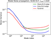 |
Fig. 16 Same as Fig. 15 with the x-axis in log scale. |
| In the text | |
|
Fig. 17 Gain with respect to the PWS as a function of corrected modes for the SCAO/ELT configuration (3000 modes, a 2λ/D modulation radius, sharp-Bi–O edge, and grey Bi–O edge). |
| In the text | |
|
Fig. 18 SR as a function of flux for the SCAO/ELT configuration (3000 modes, 2λ/D modulation radius). |
| In the text | |
Current usage metrics show cumulative count of Article Views (full-text article views including HTML views, PDF and ePub downloads, according to the available data) and Abstracts Views on Vision4Press platform.
Data correspond to usage on the plateform after 2015. The current usage metrics is available 48-96 hours after online publication and is updated daily on week days.
Initial download of the metrics may take a while.