| Issue |
A&A
Volume 687, July 2024
|
|
|---|---|---|
| Article Number | A202 | |
| Number of page(s) | 8 | |
| Section | Astronomical instrumentation | |
| DOI | https://doi.org/10.1051/0004-6361/202349118 | |
| Published online | 15 July 2024 | |
Transformer neural networks for closed-loop adaptive optics using nonmodulated pyramid wavefront sensors★
1
School of Electrical Engineering, Pontificia Universidad Católica de Valparaíso,
Valparaíso,
Chile
e-mail: This email address is being protected from spambots. You need JavaScript enabled to view it.
2
Aix Marseille Univ, CNRS, CNES, LAM,
Marseille,
France
Received:
28
December
2023
Accepted:
30
April
2024
Abstract
Context. The pyramid wavefront sensor (PyWFS) provides the required sensitivity for demanding future adaptive optics (AO) instruments. However, the PyWFS is highly nonlinear and requires the use of beam modulation to successfully close an AO loop under varying atmospheric turbulence conditions. This comes at the expense of a loss in sensitivity.
Aims. We trained, analyzed, and compared the use of deep neural networks (NNs) as nonlinear estimators for the nonmodulated PyWFS, identifying the most suitable NN architecture for a reliable closed-loop AO.
Methods. We developed a novel training strategy for NNs that seeks to accommodate for changes in residual statistics between open and closed loops, plus the addition of noise for robustness purposes. Through simulations, we tested and compared several deep NNs from classical to new convolutional neural networks (CNNs), plus the most recent transformer neural network (TNN; global context visual transformer, GCViT), first for an open loop and then for a closed loop. By identifying and properly retraining the most adequate deep neural net, we tested its simulated performance first in an open loop and then for closing an AO loop at a variety of noise and turbulence conditions. We finally tested the trained NN ability to close a real AO loop for an optical bench.
Results. Using open-loop simulated data, we observe that a TNN (GCViT) largely surpasses any CNN in estimation accuracy in a wide range of turbulence conditions. Moreover, the TNN performs better in a simulated closed loop than CNNs, avoiding estimation issues at the pupil borders. When closing the loop at strong turbulence and low noise, the TNN using nonmodulated PyWFS data is able to close the loop, similar to a PyWFS with 12λ/D of modulation. When the noise is increased, only the TNN is able to close the loop, while the standard linear reconstructor fails even when a modulation is introduced. Using the GCViT, we closed a real AO loop in the optical bench and achieved a Strehl ratio between 0.28 and 0.77 for turbulence conditions corresponding to Fried parameters ranging from 6 to 20 cm, respectively.
Conclusions. Through a variety of simulated and experimental results, we demonstrate that a TNN is the most suitable architecture for extending the dynamic range without sacrificing sensitivity for a nonmodulated PyWFS. It opens the path for using nonmodulated Pyramid WFSs in an unprecedented range of atmospheric and noise conditions.
Key words: instrumentation: adaptive optics
The movies associated to Figs. 7 and 9 are available at https://www.aanda.org
© The Authors 2024
 Open Access article, published by EDP Sciences, under the terms of the Creative Commons Attribution License (https://creativecommons.org/licenses/by/4.0), which permits unrestricted use, distribution, and reproduction in any medium, provided the original work is properly cited.
This article is published in open access under the Subscribe to Open model. This email address is being protected from spambots. You need JavaScript enabled to view it. to support open access publication.
1 Introduction
The world will see the arrival of extremely large telescopes (ELTs) with primary mirror diameters larger than 25 m within the next ten years. However, atmospheric turbulence affects light propagation, acting as a dynamic phase mask that introduces aberrations to the optical path. This finally diminishes the ability of current large telescopes, as well as future ELTs, to properly focus light at the diffraction limit. Adaptive optics (AO; Roddier 1999) can assist modern telescopes in overcoming atmospheric turbulence, first, by measuring and estimating the wavefront fluctuations from reference sources, and then optically compensating for the aberrations before the science instruments are reached. Over the past 25 yr, AO has revolutionized astronomy by providing the highest achievable image quality for ground-based observatories, becoming a fundamental component in the upcoming ELTs from first light (Hippler 2019).
Wavefront sensors (WFSs) are the core of modern AO systems. Basically, a WFS needs to perform measurements quickly enough (often within a millisecond) to infer the dynamic phase aberrations present in the wavefront that passes through the atmosphere on its way to the telescope. Thus, an AO loop can use a deformable mirror to compensate for the atmospheric turbulence in real time. Of the known WFSs, the pyramid wavefront sensor (PyWFS; Ragazzoni 1996) exhibits relevant performance advantages such as high sensitivity, high spatial frequencies, and a reduced noise propagation (Fauvarque et al. 2016; Chambouleyron, V. et al. 2023). It was therefore successfully implemented in current large telescopes (Large Binocular Telescope, LBT, Esposito et al. 2010, Subaru, Guyon et al. 2020, and Keck, Mawet et al. 2022) and it is being considered for the next-generation ELT instruments (HARMONI, Neichel et al. 2022 and MICADO, Clénet et al. 2022).
The PyWFS places the apex of a pyramidal four-sided prism at the point spread function (PSF) plane (focal plane) of the incoming wavefront, finally reimaging four different version of the pupil projected onto a detector array. Then, the slopes of the wavefront can be easily estimated from the measured image, although the PyWFS finally offers a very limited dynamic range where its response is still linear (Vérinaud 2004; Burvall et al. 2006), despite its superb sensitivity. In practical scenarios, and as suggested in the seminal work done by Ragazzoni (1996), the inherent nonlinearity of the PyWFS can be counteracted by circularly modulating the incoming beam over the apex of the pyramid, which homogenizes the illumination of the four sides of the prism. Although the linearity is improved, beam modulation comes with a detrimental effect on the sensitivity, plus the need for additional fast and expensive optomechanical elements. The nonlinearity of the PyWFS becomes evident when using linear matrix-based reconstruction models (Korkiakoski et al. 2007). Despite several efforts in the literature to use nonlinear least-squares methods, which are often iterative, such as in Frazin (2018); Shatokhina et al. (2020); Hutterer et al. (2023), alternative approaches also exploit the compensation of the optical gains (OG) based on the turbulence statistics (Deo, et al. 2019; Chambouleyron, et al. 2020). Nevertheless, OG compensation is only a first-order approximation of the nonlinearities (Deo, et al. 2019), being particularly hard to handle for the nonmodulated PyWFS case.
Neural networks (NNs), and more particularly, deep NNs, which make use of a larger number of hidden layers and intricate interconnections, are a great asset today for solving a variety of hard nonlinear problems in imaging, such as detection, classification, and inference (LeCun et al. 2015). This also holds for WFSs, for which Nishizaki et al. (2019) demonstrated that any imaging system can be turned into an image-based WFS by appropriately training a convolutional neural network (CNN) to infer the Zernike modal approximation of the incoming wave-front. Since then, deep learning has been applied to improve the estimation performance of focal-plane WFSs (Orban de Xivry et al. 2021), Shack-Hartmann WFSs (DuBose et al. 2020), phase-diversity-based WFSs (Andersen et al. 2020), Lyot-based WFSs (Allan et al. 2020), and also the PyWFS (Landman & Haffert 2020), for which a CNN was used jointly with the linear estimator to improve the PyWFS linearity. Recently, Wong et al. (2023) demonstrated that a three-layer fully connected neural network can estimate low-order modes from a PyWFS with and without modulation, while Archinuk et al. (2023) used a simple CNN to estimate the first 400 modes from the nonmodulated PyWFS. Since AO is a two-stage process of wavefront sensing and wave-front control, we can also use deep NNs not only to improve the accuracy of the wavefront estimation of the WFS, but also to improve the performance of the closed-loop AO system, as proposed in Nousiainen et al. (2021) and Pou et al. (2022), who used reinforcement learning.
Most of the deep-learning WFSs have adapted conventional deep neural nets that were originally developed for computer vision applications, such as Xception (Chollet 2017), VGG–Net (Simonyan & Zisserman 2014), or ResNet (He et al. 2016), while Vera et al. (2021) crafted an original deep neural net (WFNET) for image-based WFSs. Nevertheless, there is a new generation of CNNs, ConvNeXt and ConvNeXt v2 (Liu et al. 2022; Woo et al. 2023), that delivers an impressive performance in classification tasks. Moreover, there is a new class of deep neural nets, called transformer neural networks (TNN), that outperforms classical CNNs for a variety of vision applications. These nets are the visual transformer ViT (Dosovitskiy et al. 2020) and the global context visual transformer GCViT (Hatamizadeh et al. 2022), which currently are the latest developments. Instead of convolutions, TNNs such as the GCViT can find correlations between image patches and their influence on the target outputs. Nevertheless, the main disadvantage of most modern CNNs and TNNs is that they often require massive numbers of data for the training, although they can be efficiently retrained and do not need to start from scratch.
A good wavefront estimator or reconstructor will necessarily lead to a good AO performance. Therefore, this we studied and analyzed the use of deep neural nets as a nonlinear estimator for the nonmodulated PyWFS, enabling a reliable open- and closed-loop adaptive optics performance. To do this, we tested and compared the ability of several conventional and newest neural network architectures to handle the PyWFS nonlinearity, developing appropriate training strategies to accommodate for changes in residual statistics between open and closed loop. By choosing and properly training the most adequate deep neural net for the task, we demonstrate that the dynamic range of the nonmodulated PyWFS can be extended without sacrificing sensitivity, enabling closed-loop operations at a variety of noise and turbulence conditions without beam modulation.
2 Method
In this section, we describe the methods we used to (1) simulate the PyWFS forward model under a variety of turbulence and noise conditions, (2) train the deep neural networks using open-loop data, (3) retrain closed-loop scenarios, (4) determine the metrics to quantifying the performance of the different NN estimators, and (5) to configure the experimental setup.
2.1 Simulation framework
We used the OOMAO toolbox (Conan & Correia 2014), written in Matlab, to generate the incoming aberrated wavefronts and simulate the propagation through the PyWFS up to the detector plane. The phase-map dataset was generated with a spatial resolution of 268 × 268 pixels for a telescope with an aperture of 1.5 m working at λ = 550 nm with an r0 distribution ranging from 1cm to 20 cm (distributed in discrete steps of 2 cm after 2 cm), leading to an effective D/r0 range between 7.5 and 150. It is important to note that as D/r0 increases, the turbulence becomes stronger. For every phase map, we retrieved the first 209 Zernike coefficients, ignoring piston, which were considered as the ground truth for estimation purposes. After propagating each phase map for an incoming magnitude 0 light source in the V band using OOMAO, we stored the intensity image I projected on the WFS detector of size 268 × 268 pixels with an exposure time of 1 sec without noise. The diameter of each subpupil at the simulated WFS detector spanned 68 pixels. In total, the open-loop phase-map dataset was comprised of 210 000 uncorrelated samples (phase map, Zernikes, and PyWFS image) obtained from random turbulence realizations given the selected D/r0 level.
We also simulated phase-map sequences (using two layers moving at 5 and 10 ms−1 sampled at 250 Hz) of 1000 samples for different turbulence strengths and several levels of modulation for the PyWFS at 0λ/D (nonmodulated), 3λ/D, 5λ/D, and 12λ/D. These sequences were made for the closed-loop testing.
2.2 Magnitude and noise
We added noise to the intensity image I on demand as required by either the training or testing stage. By fixing the telescope size to 1.5 m, we first scaled the image to a proportional photon flux depending on the magnitude of the star (Mag) and the exposure time (Te), such that
 (1)
(1)
Then, we applied Poisson noise to the scaled measurement Iref, leading to the noisy image Inoise, enabling the calculation of the effective signal–to–noise ratio (S/N) defined as
 (2)
(2)
Figure 1 displays the example of three images measured by the PyWFS for different stellar magnitudes at a fixed exposure time, with the respective associated S/N. The image clearly degrades as the photon flux diminishes. Before it was used with the linear or NN estimators, the noisy PyWFS measurement was always normalized. Throughout the paper, we only refer to the S/N level of the measurements when dealing with noise.
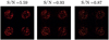 |
Fig. 1 Nonmodulated PyWFS measurement for different stellar magnitudes at a fixed exposure leading to different effective S/N levels. |
2.3 Neural network training
We selected four deep neural network architectures as nonlinear estimators for the nonmodulated PyWFS. Xception (Nishizaki et al. 2019), WFNet (Vera et al. 2021), ConvNext (Liu et al. 2022), and GCVit (Hatamizadeh et al. 2022) were implemented in PyTorch and adapted to perform regression at the last layer to provide simultaneous estimates for the first 209 Zernike modes (without piston).
Since all implemented NNs accept the same input image size from the PyWFS and deliver estimates of the Zernike coefficients with the same number of coefficients as well, then all NNs were trained and tested with the exact same portions of the simulated dataset, which was divided into 75% for training and 25% for testing. All training sessions were performed in PyTorch by using 8 NVIDIA Quadro RTX5000 GPUs. From several preliminary tests on the NNs, we realized that the choice of a proper range of values for the learning rate and a suitable loss function heavily depend on the strength and number of Zernikes modes to be estimated, which are also related to the turbulence strength. A loss function is an error metric that is computed between the estimated output values of the NN (in this case, a vector of Zernike coefficients  ) and the vector of ground-truth values (z) used for training. The most common loss functions are the mean square error (MSE) and the mean absolute error (MAE), defined as
 (3)
(3)
where Ν is the number of coefficients. On the other hand, the learning rate is the weight given to the calculated loss function that is back-propagated to update the NN hidden parameters at every training iteration. For instance, mixing a high learning rate (larger than 10−5) with the MAE loss function allows a correct training of low-order, high-amplitude Zernikes modes. In contrast, mixing a low learning rate (≈10−6 or lower) with the MSE improves the training of high-order, low-amplitude Zernikes modes.
Therefore, we generated a two-step training strategy for open-loop wavefronts, creating two training datasets with different distributions for the Zernike modes, as shown in Fig. 2. The first training uses a limited dataset with a range between D/r0 = 25 and 150, a starting learning rate of 10−5, and MAE as the loss, which emphasizes a boost in the linearity response of the nonmodulated PyWFS. Then, in the second stage, we retrained the NNs using the whole dataset from D/r0 = 7.5 to 150, a starting learning rate of 10−6, and MSE as the loss, which played a significant role in preserving the sensitivity of the PyWFS.
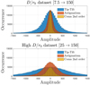 |
Fig. 2 Amplitude distribution for selected Zernike modes for two turbulence training regimes. The full range of 7.5 > D/r0 > 150 is shown at the top, and the high range of 25 > D/r0 > 150 is shown at the bottom. |
2.4 Closed-loop training
After training the NNs to properly estimate the output from a nonmodulated pyramid for a variety of turbulence conditions in open loop, we devised a retraining strategy to prepare for the statistics of the residuals in closed-loop. We propose a two-step approach as depicted in Fig. 3. In the first step, we input a phase map from the dataset to the PyWFS and estimate the Zernike coefficients from the chosen NN architecture. Then, we reconstruct the estimated phase out from the Zernike coefficients and compute the phase residual by plain subtraction. In the second step, we input the phase residual to the PyWFS and estimate a new set of Zernike coefficients using the NN. We then calculate the loss function MAE for the estimated residual coefficients, and update the parameters of the NN with a learning rate of 10−6.
This novel training approach for closed-loop measurements allowed us to use the simulated wavefronts in the dataset independently, regardless of whether they were correlated in time. The proposed scheme serves as an effective data-augmentation approach, which leads to a higher diversity in the statistics provided for the NN models.
In our initial training using closed-loop data, we considered an ideal noiseless case. Nonetheless, when we prepared an NN for a more realistic scenario, we retrained the NN by randomly selecting an S/N level for the PyWFS measurement (between S/N = 0.7 and S/N = 7), which tended to improve the robustness of the trained NNs (Bishop 1995).
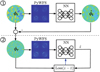 |
Fig. 3 Neural network closed-loop training strategy. The first stage uses the estimate by the NN from open-loop data to compute a residual phase that is used as the input for the second stage. The Zernike coefficients of the residual are used as the ground truth to compute the loss function used to retrain the NN. |
2.5 Performance metrics
To compare the open-loop wavefront estimate accuracy of the different NNs in simulations, we used the root mean square error (RMSE) of the predicted Zernike coefficients as follows:
 (4)
(4)
where ɀ corresponds to the ground-truth Zernike coefficients extracted from the incoming wavefront ϕi,  are the Zernike coefficients estimated by the NN, and Ν is the number of Zernike coefficients.
When we switched to closed loop in the simulations, we analyzed the standard deviation of the phase-map residual σϕ. The residual was computed by the difference between the incoming phase ϕi and the corresponding update given by the last reconstruction from the last estimated Zernike coefficients.
For the experimental validation, we also analyzed the system performance by computing the Strehl ratio given by the ratio of the maximum value of the reconstructed PSF and the maximum value of the equivalent diffraction-limited PSF.
2.6 Experimentai adaptive optics bench
We used the PULPOS AO bench (Tapia et al. 2022) to validate the performance of the PyWFS + GCVIT in closed loop. The particular branch of PULPOS used to close the AO loop with a PyWFS is shown in Fig. 4. We used a λ = 635 nm fiber-coupled laser source (Thorlabs S1FC635) attached to an air-spaced doublet collimator (Thorlabs F810APC-635) and a beam expander (Thorlabs GBE02-A). After a 5 mm diameter aperture stop (P), the beam passes through a 4f-system with 1X magnification (L1 and L2) before reaching the reflective high-speed spatial light modulator (SLM; Meadowlark HSP1920-488-800-HSP8, 1920 × 1152 pixels, 9.2 µm pixel size), where phase maps of 560 × 560 pixels are projected to emulate the desired turbulence, matching the pupil size relayed at the SLM. Then, a beam splitter (BS1) redirects the aberrated wavefront through a 0.75X magnification 4f-system (L3 and L4), reaching the L5 lens (400 mm) that focuses the beam on the PSF plane where the apex of a zeonex pyramid is located. Then, the L6 lens (200 mm) colli-mates the four subpupils emerging from the pyramid, projected onto a high-speed CMOS camera (Emergent Vision HR-500-S-M, 9 µm pixel size, 1586 fps, 812 × 620 pixels). The WFS images were cropped at 620 × 620 pixels, where each of the subpixels spanned a diameter of 110 pixels. These images were resized to match the subpixel diameter of the pupils used in the simulations before entering the NN estimation. In parallel, we recorded the PSF that was imaged by a 125 mm lens onto the science camera (SC; Emergent Vision HR-500-S-M, 9 µm pixel size), where we extracted the Strehl ratio. The SLM and cameras were controlled by a desktop computer loaded with an RTX4000 GPU.
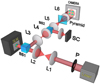 |
Fig. 4 Schematic of the experimental AO setup using PULPOS to test the PyWFS in open and closed loop. |
3 Results
In this section, we list the results we obtained in open and closed loop using simulations of the nonmodulated PyWFS estimated with a variety of deep NN options. These results then drove the selection of the best-performing NN architecture, which was used in the final experimental validation using PULPOS in open and closed loop as well.
3.1 Neural network comparison
In our initial test results, we evaluated the performance of several deep NNs trained with identical parameters using the entire dataset range (r0 = [1 → 20] cm). The chosen NNs were three CNNs, Xception, WFNet, and ConvNext, and one TNN, GCViT. In particular, we trained the light-weight version of the GCViT, which is the GCViT-xxtiny.
In Table 1, we present a summary of the number of parameters, the estimation speed for the same training computer machine using a single GPU card, and the estimation performance (average fitting error per mode) from noiseless measurements of every tested NN architecture. The number of parameters refers to the number of interconnections (weights) inside each NN, which depends on the number of layers and neurons of each architecture and is strongly correlated to the size of the NN stored in the GPU memory. However, every architecture has its own intricacies and choice for the number of hidden layers and the inner operators such as linear convolutions and neuron nonlinearities that finally affect the speed of calculus of each NN in a different manner.
The results clearly show that the GCViT achieves the best average performance, meaning that it is able to provide good estimates in the whole turbulence range. A slightly worse performance is surprisingly achieved by the Xception, although it is an older CNN than the newer ConvNext. The worst performance was achieved by the WENet, which may be related to the fact that it was originally developed for undersampled image-based WES. Interestingly, the error was somewhat proportional to the number of parameters of the NNs. Nevertheless, the GCViT seems to be slowest even though it has fewer parameters. One possible explanation for this is that it is far more intricate and has a more complicated architecture.
To select the most promising NN candidate for real AO applications, we tested the two best-performing NNs in closed loop, the Xception as the CNN candidate and the GCViT as the TNN candidate. We performed the close-loop test under a frozen turbulence condition (static phase map at the input) and no noise (S/N = ∞) to analyze their estimation and compensation behavior in ideal conditions. The closed-loop results for a turbulence of D/r0 = 75 are depicted in Fig. 5. Both NNs quickly reduce the residual within a few frames. Nevertheless, at some point, the CNN tends to diverge as the TNN approaches the ideal residual value for the estimation of 209 Zernike modes. This problem for the the CNN in closed loop is clearly seen after inspecting the residual phase map, where significant aberrations start to appear at the borders, most likely created by a deficient estimation of the high-order modes by the CNN.
This behavior of the CNN is probably due to the convolu-tional nature of the CNN, which may complicate the handling of the phase at the sharp pupil borders. On the other hand, the TNN can identify the portions within the image that are informative, which may explain its superior performance, delivering a spatially homogeneous residual phase map. As a side note, we caution that it is impossible to close the loop using a linear estimator for the nonmodulated PyWFS at this turbulence level.
Comparison of deep neural networks used for WFS in terms of the number of parameters (# Params), inference speed (Speed), and estimation error (Error).
3.2 Noise response
After we decided that the GCViT is the most suitable NN architecture for closing the loop with a nonmodulated PywFS, we retrained the GCViT with different levels of photon noise equivalent to a range of S/N between 0.7 and 7, randomly applied to the measurements. We compared the GCViT estimate with the linear estimate of the nonmodulated PyWFS for a turbulence range between D/r0 = 7.5 and D/r0 = 150 in open loop. The performance results for measurements taken with two noise levels (low noise (S/N = 7) and high noise (S/N = 0.7)) are presented in Fig. 6. The first observation is that the linear estimate for the nonmodulated PyWFS is extremely immune to noise given its high sensitivity, so that the two plots are merged into one.
For a high S/N, the GCViT is vastly superior to the linear estimate in the whole turbulence range, clearly improving the linearity of the PyWFS response, particularly within the D/r0 = 20–60 range. Although the GCViT estimates are still better than the traditional linear estimation for the PyWFS under low S/N conditions for most of the turbulence range, the linearity advantages are not as high as in the high S/N case. Nevertheless, the estimation for the GCViT can become slightly worse than the linear estimate for the PyWFS for very weak turbulence at D/r0 = 7.5.
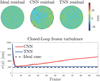 |
Fig. 5 Closed-loop performance in simulations using a constant input phase with two neural networks, a CNN (Xception) and a TNN (GCViT). Top: last frame of the closed-loop residual phase map. Bottom: evolution of the residual standard deviation, comparing the CNN, TNN, and the optimal estimation of 209 Zernike modes. |
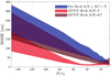 |
Fig. 6 Open-loop performance comparison in simulations for the linear least-squares estimate and the GCViT estimate for a nonmodulated PyWFS at different S/N. |
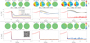 |
Fig. 7 Closed-loop residual phase evolution using simulated data at D/r0 = 150 (top column) and D/r0 = 15 (bottom row), comparing the linear least-squares estimate for the PyWFS at different modulation levels (M = 3,5 and 12λ/D) against the GCViT estimate for the nonmodulated PyWFS (M = 0). The AO loop is closed at frame 100 using a proportional controller with gain k = 0.5. From left to right: results for different S/N levels. At the top of each plot, we show the residual phase for the different estimation methods at frame 250. The movies are available online. |
3.3 Closed-loop performance
We tested the performance of the GCViT trained with noise when closing an AO loop using the nonmodulated PyWFS. We compared the closed-loop performance against the PyWFS working at different modulations of 3λ/D, 5λ/D, and 12λ/D, using the traditional linear least-squares estimator. We chose to close the AO loop at weak turbulence conditions of D/r0 = 15 as well as at the worst trained turbulence conditions of D/r0 = 150, where it is impossible to close the loop with the nonmodulated PyWFS using linear estimation. In Fig. 7 we present the results for closing the AO loop for three different S/N levels: 9.04, 1.41, and 0.57. The lowest S/N level is beyond the training regime used for the GCViT.
The AO loop was closed at frame 100. For the strong-turbulence case (shown in the top row), all the WFSs are able to close the loop for all high S/N and reach a stable but different residual levels. The GCViT and the PyWFS at 12λ/D using the linear estimate perform best, indicating that they may share an equivalent linear response at this turbulence regime, as corroborated by the very similar residual shape for the very last frame. As the S/N decreases, only the GCViT is able to maintain a similar level of residual as obtained in high S/N conditions, while the PyWFS using linear estimation at different modulations fails to close the loop. Only at the very lowest S/N level does the GCViT show some slight difficulties in maintaining the expected residual levels achieved for higher S/N, but without loosing the ability of closing the loop at all. By being able to close the loop in this extreme turbulence regime even at high noise levels, it seems that by using the nonmodulated PyWFS measurements, the GCViT is able to keep some of the inherent high sensitivity while still dramatically increasing the linearity. The bottom row of Fig. 7 reveals the results for a weak-turbulence regime, where the GCViT shows a similar behavior, perhaps slightly worse in terms of residuals, successfully closing the AO loop as all the modulated PyWFS versions for the high S/N scenario. However, as the S/N decreases, the loss of sensitivity for the PyWFS is clear as modulation is increased at 12λ/D, while the GCViT is able to maintain a stable residual in between of the PyWFS at 3λ/D and 5λ/D of modulation for the lowest S/N case.
3.4 Experimental validation
We used the PULPOS (Tapia et al. 2022) AO bench to obtain measurements from the nonmodulated PyWFS under controlled, arbitrary phase maps projected onto the SLM display. We started by calibrating the PyWFS and obtaining the interaction matrix by projecting the first pure 209 Zernike modes (without piston) in push and pull using an amplitude of 0.5/λ. As a first part of the experimental validation, we tested the PyWFS using the same open-loop dataset as in the simulations, although only for r0 = [6 → 20] cm, which are the conditions found at the 1.5 m telescope at the Observatoire de Haute-Provence (OHP) that is currently running PAPYRUS (Muslimov et al. 2021), an adaptive optics instrument based on a PyWFS. We present the performance results for the classical linear estimation method and the GCViT in Fig. 8, comparing both the use of simulated measurements and the experimental PyWFS data obtained at PULPOS. The GCViT has only be trained using simulated data.
The plots in Fig. 8 show that the GCViT estimation using experimental data vastly outperforms the classical least-squares estimation, as predicted by the simulations. Despite some general offset in both cases, the experimental estimates follow the overall trend and standard deviation obtained when using the simulated measurements. The linearity offered by the GCViT estimates using the nonmodulated PywFS are superior to what is being offered by the linear estimation methods. In addition, we may even consider that the sensitivity offered by the GCViT is also better, considering the superior performance at low turbulence levels and that measurements are noisy since the CMOS camera that was used for the PyWFS is not a science-grade camera.
As the second part of the experimental validation, we used the trained GCViT to close an AO loop using PULPOS with the nonmodulated PyWFS. We estimated the 209 Zernike modes on the fly using an NVIDIA RTX4000 GPU. As a deformable mirror, we used the same SLM with which we projected the aberrated turbulence phase maps in open loop, now displaying the compensated phase maps given by the chosen control law applied to the estimates provided by the GCViT. Although the simulated phase-map sequence used for closed loop is sampled at 250 Hz, we close the AO loop in PULPOS at 10 Hz because we work on a real-time control upgrade. We chose to close the loop at three representative turbulence conditions with r0 at 6, 10, and 20 cms, equivalent to a D/r0 of 25, 15, and 7.5 at OHP, respectively. The results displaying the evolution of the Strehl ratio computed from the instantaneous PSFs captured by the scientific camera in PULPOS for different turbulence conditions are shown at the top of Fig. 9, where we close the loop at frame 100. By using the GCViT, we are clearly able to close the AO loop in all situations, and the loop is stable. As a side note, we can hardly close the loop at D/r0 = 7.5 when using linear estimation with the nonmodulated pyramid in the AO bench, which explains why these results are not even presented here.
We display at the bottom of Fig. 9 the PSFs and respective central horizontal line profiles, integrated between frames 100 and 300, as obtained by the GCViT in closed loop for different turbulence conditions, corresponding to an average Strehl ratio of 0.28, 0.56, and 0.77 for an r0 of 6, 10, and 20cm, respectively.
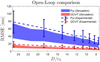 |
Fig. 8 Comparison of the wavefront estimation error using least-squares estimation (Pyr) and the GCViT estimation for simulated and experimental open-loop measurements from a nonmodulated PyWFS. |
4 Conclusions
We presented a comparative analysis of using deep neural networks as nonlinear estimators for the nonmodulated PyWFS. We trained, tested, and compared several conventional and most advanced neural network architectures to handle the PyWFS nonlinearity, where convolutional neural networks have been used most widely for WFS applications so far. We developed a novel training strategy that combines the use of open- and closed-loop data, as well as the addition of noise for robustness purposes. Through simulations, we found that a modern TNN, in this case, the GCViT, is the most suitable NN architecture for a closed-loop AO operation, avoiding systematic phase estimation problems at the pupil borders caused by the convolutional nature of CNNs.
When testing in open loop, the GCViT was able to dramatically extend the dynamic range of the nonmodulated PyWFS in contrast with the traditional linear estimation methods for a variety of noise conditions, although there is a clear loss in performance at very high noise levels. However, when testing in a simulated AO scenario at the worst turbulence conditions, we found that the GCViT is able to close a stable AO loop similar to a modulated PyWFS at 12λ/D at a high S/N level. Moreover, the GCViT is very robust to noise: It was the only estimator able to reliably close the AO loop for medium to low S/N for strong turbulence conditions. For weak turbulence, the GCViT was able to close the loop for the whole range of S/N, with a performance similar to the PyWFS with 5λ/D of modulation. These results were experimentally validated in the PULPOS AO bench, where the GCViT was able to consistently close the AO loop for turbulence ranging from 6 cm to 20 cm, achieving an integrated Strehl ratio at the scientific camera between 0.28 and 0.77, respectively.
In conclusion, we demonstrated that a TNN such as the GCViT can be properly trained and become suitable as a nonlinear estimator for a nonmodulated PyWFS. By dramatically extending the dynamic range of the nonmodulated PyWFS without sacrificing sensitivity, the GCViT can be used in real AO scenarios, being robust to noise and varying turbulence conditions. This paves the way for further testing in real observing conditions, which is beyond the scope for this work. It is interesting that the proposed NN was trained entirely offline. The experimental results we presented showed that the trained TNN possesses a certain degree of flexibility to accommodate statistical variations. Nevertheless, a retraining using real data may be necessary in some cases, which will be validated through on-sky experiments at OHP using the PAPYRUS instrument (Chambouleyron et al. 2022). This is scheduled for mid 2024.
As prospective work, the results obtained at D/r0 = 150 are very encouraging to scale and extend our research toward ELTs, which means orders-of-magnitude more Zernike modes and larger D/r0 turbulence ranges. This can also benefit from the design and use of modern optical preconditioners (Guzmán et al. 2024) to improve the dynamic range of the non-modulated PyWFS even further. Moreover, we may extend our work to detecting differential piston modes between the ELT segments (petal modes) using the nonmodulated pyramid (Levraud et al. 2022), while also adapting the GCViT for improving the wavefront estimation performance of an even more sensitive WFS such as the Zernike WFS (Cisse et al. 2022).
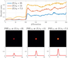 |
Fig. 9 Experimental closed-loop performance for different turbulence conditions using GCViT with a nonmodulated PyWFS. The AO loop is closed at frame 100 (gain k = 0.3). Top: evolution of the Strehl ratio for different turbulence conditions. Bottom: integrated PSFs in closed loop (PSFCL) with their respective horizontal line profiles. The movies are available online. |
Supplementary Material
Movie 1 associated with Fig. 7 Access Supplementary Material
Movie 2 associated with Fig. 7 Access Supplementary Material
Movie 3 associated with Fig. 7 Access Supplementary Material
Movie 4 associated with Fig. 7 Access Supplementary Material
Movie 5 associated with Fig. 7 Access Supplementary Material
Movie 6 associated with Fig. 7 Access Supplementary Material
Movie 1 associated with Fig. 9 Access Supplementary Material
Movie 2 associated with Fig. 9 Access Supplementary Material
Movie 3 associated with Fig. 9 Access Supplementary Material
Acknowledgements
The authors gratefully acknowledge the financial support provided by Agencia Nacional de Investigacion y Desarrollo (ANID) ECOS200010, STIC2020004, ANILLOS ATE220022, BECA DOCTORADO NACIONAL 21231967; Fondos de Desarrollo de la Astronomía Nacional (QUIMAL220006, ALMA200008); Fondo Nacional de Desarrollo Cientí-fico y Tecnológico (FONDECYT) (EXPLORACION 13220234, Postdoctorado 3220561); French National Research Agency (ANR) WOLF (ANR-18-CE31-0018), APPLY (ANR-19-CE31-0011), LabEx FOCUS (ANR-11-LABX-0013); Programme Investissement Avenir F-CELT (ANR-21-ESRE-0008), Action Spécifique Haute Résolution Angulaire (ASHRA) of CNRS/INSU co-funded by CNES, ORP-H2020 Framework Programme of the European Commission’s (Grant number 101004719), Région Sud and the french government under the France 2030 investment plan, as part of the Initiative d’Excellence d’Aix-Marseille Université A*MIDEX, program number AMX-22-RE-AB-151.
References
- Allan, G., Kang, I., Douglas, E. S., Barbastathis, G., & Cahoy, K. 2020, Opt. Express, 28, 26267 [NASA ADS] [CrossRef] [Google Scholar]
- Andersen, T., Owner-Petersen, M., & Enmark, A. 2020, J. Astron. Telesc. Instrum. Syst., 6, 034002 [Google Scholar]
- Archinuk, F., Hafeez, R., Fabbro, S., Teimoorinia, H., & Véran, J.-P. 2023, arXiv e-prints [arXiv:2305.09005] [Google Scholar]
- Bishop, C. M. 1995, Neural Networks for Pattern Recognition (Oxford: Oxford university press) [Google Scholar]
- Burvall, A., Daly, E., Chamot, S. R., & Dainty, C. 2006, Opt. Express, 14, 11925 [NASA ADS] [CrossRef] [Google Scholar]
- Chambouleyron, V., Fauvarque, O., Janin-Potiron, P., et al. 2020, A&A, 644, A6 [EDP Sciences] [Google Scholar]
- Chambouleyron, V., Boudjema, I., Fétick, R., et al. 2022, SPIE, 12185, 121856T [Google Scholar]
- Chambouleyron, V., Fauvarque, O., Plantet, C., et al. 2023, A&A, 670, A153 [NASA ADS] [CrossRef] [EDP Sciences] [Google Scholar]
- Chollet, F. 2017, in Proceedings of the IEEE conference on computer vision and pattern recognition, Xception: Deep Learning with Depthwise Separable Convolutions, 1800 [Google Scholar]
- Cisse, M., Chambouleyron, V., Fauvarque, O., et al. 2022, SPIE, 12185, 258 [Google Scholar]
- Clénet, Y., Buey, T., Gendron, E., et al. 2022, SPIE, 12185, 1512 [Google Scholar]
- Conan, R., & Correia, C. 2014, SPIE, 9148, 2066 [NASA ADS] [Google Scholar]
- Deo, V., Gendron, É., Rousset, G., et al. 2019, A&A, 629, A107 [NASA ADS] [CrossRef] [EDP Sciences] [Google Scholar]
- Dosovitskiy, A., Beyer, L., Kolesnikov, A., et al. 2020, arXiv e-prints [arXiv:2010.11929] [Google Scholar]
- DuBose, T. B., Gardner, D. F., & Watnik, A. T. 2020, Opt. Lett., 45, 1699 [NASA ADS] [CrossRef] [Google Scholar]
- Esposito, S., Riccardi, A., Fini, L., et al. 2010, SPIE, 7736, 107 [Google Scholar]
- Fauvarque, O., Neichel, B., Fusco, T., Sauvage, J.-F., & Girault, O. 2016, Optica, 3, 1440 [Google Scholar]
- Frazin, R. A. 2018, J. Opt. Soc. Am. A, 35, 594 [NASA ADS] [CrossRef] [Google Scholar]
- Guyon, O., Lozi, J., Vievard, S., et al. 2020, SPIE, 11448, 468 [Google Scholar]
- Guzmán, F., Tapia, J., Weinberger, C., et al. 2024, Photon. Res., 12, 301 [CrossRef] [Google Scholar]
- Hatamizadeh, A., Yin, H., Heinrich, G., Kautz, J., & Molchanov, P. 2022, arXiv e-prints [arXiv:2206.09959] [Google Scholar]
- He, K., Zhang, X., Ren, S., et al. 2016, in Proceedings of the IEEE conference on computer vision and pattern recognition, Deep Residual Learning for Image Recognition, 770 [Google Scholar]
- Hippler, S. 2019, J. Astron. Instrum., 08, 1950001 [CrossRef] [Google Scholar]
- Hutterer, V., Neubauer, A., & Shatokhina, J. 2023, Inverse Prob., 39, 035007 [NASA ADS] [CrossRef] [Google Scholar]
- Korkiakoski, V., Vérinaud, C., Louarn, M. L., & Conan, R. 2007, Appl. Opt., 46, 6176 [NASA ADS] [CrossRef] [Google Scholar]
- Landman, R., & Haffert, S. Y. 2020, Opt. Express, 28, 16644 [NASA ADS] [CrossRef] [Google Scholar]
- LeCun, Y., Bengio, Y., & Hinton, G. 2015, Nature, 521, 436 [Google Scholar]
- Levraud, N., Chambouleyron, V., Fauvarque, O., et al. 2022, SPIE, 12185, 1622 [Google Scholar]
- Liu, Z., Mao, H., Wu, C.-Y., et al. 2022, arXiv e-prints [arXiv:2201.03545] [Google Scholar]
- Mawet, D., Fitzgerald, M. P., Konopacky, Q., et al. 2022, SPIE, 12184, 599 [Google Scholar]
- Muslimov, E., Levraud, N., Chambouleyron, V., et al. 2021, SPIE, 11876, 56 [Google Scholar]
- Neichel, B., Fusco, T., Sauvage, J.-F., et al. 2022, SPIE, 12185, 1218515 [NASA ADS] [Google Scholar]
- Nishizaki, Y., Valdivia, M., Horisaki, R., et al. 2019, Opt. Express, 27, 240 [NASA ADS] [CrossRef] [Google Scholar]
- Nousiainen, J., Rajani, C., Kasper, M., & Helin, T. 2021, Opt. Express, 29, 15327 [NASA ADS] [CrossRef] [Google Scholar]
- Orban de Xivry, G., Quesnel, M., Vanberg, P.-O., Absil, O., & Louppe, G. 2021, MNRAS, 505, 5702 [NASA ADS] [CrossRef] [Google Scholar]
- Pou, B., Ferreira, F., Quinones, E., Gratadour, D., & Martin, M. 2022, Opt. Express, 30, 2991 [NASA ADS] [CrossRef] [Google Scholar]
- Ragazzoni, R. 1996, J. Mod. Opt., 43, 289 [Google Scholar]
- Roddier, F. 1999, Adaptive Optics in Astronomy (Cambridge: Cambridge University Press) [CrossRef] [Google Scholar]
- Shatokhina, I., Hutterer, V., & Ramlau, R. 2020, J. Astron. Telesc. Instrum. Syst., 6, 010901 [CrossRef] [Google Scholar]
- Simonyan, K., & Zisserman, A. 2014, arXiv e-prints [arXiv:1409.1556] [Google Scholar]
- Tapia, J., Bustos, F. P., Weinberger, C., Romero, B., & Vera, E. 2022, SPIE, 12185, 2222 [Google Scholar]
- Vera, E., Guzmán, F., & Weinberger, C. 2021, Appl. Opt., 60, B119 [NASA ADS] [CrossRef] [Google Scholar]
- Vérinaud, C. 2004, Opt. Commun., 233, 27 [Google Scholar]
- Wong, A. P., Norris, B. R., Deo, V., et al. 2023, PASP, 135, 114501 [NASA ADS] [CrossRef] [Google Scholar]
- Woo, S., Debnath, S., Hu, R., et al. 2023, arXiv e-prints [arXiv:2301.00808] [Google Scholar]
All Tables
Comparison of deep neural networks used for WFS in terms of the number of parameters (# Params), inference speed (Speed), and estimation error (Error).
All Figures
|
Fig. 1 Nonmodulated PyWFS measurement for different stellar magnitudes at a fixed exposure leading to different effective S/N levels. |
| In the text | |
|
Fig. 2 Amplitude distribution for selected Zernike modes for two turbulence training regimes. The full range of 7.5 > D/r0 > 150 is shown at the top, and the high range of 25 > D/r0 > 150 is shown at the bottom. |
| In the text | |
|
Fig. 3 Neural network closed-loop training strategy. The first stage uses the estimate by the NN from open-loop data to compute a residual phase that is used as the input for the second stage. The Zernike coefficients of the residual are used as the ground truth to compute the loss function used to retrain the NN. |
| In the text | |
|
Fig. 4 Schematic of the experimental AO setup using PULPOS to test the PyWFS in open and closed loop. |
| In the text | |
|
Fig. 5 Closed-loop performance in simulations using a constant input phase with two neural networks, a CNN (Xception) and a TNN (GCViT). Top: last frame of the closed-loop residual phase map. Bottom: evolution of the residual standard deviation, comparing the CNN, TNN, and the optimal estimation of 209 Zernike modes. |
| In the text | |
|
Fig. 6 Open-loop performance comparison in simulations for the linear least-squares estimate and the GCViT estimate for a nonmodulated PyWFS at different S/N. |
| In the text | |
|
Fig. 7 Closed-loop residual phase evolution using simulated data at D/r0 = 150 (top column) and D/r0 = 15 (bottom row), comparing the linear least-squares estimate for the PyWFS at different modulation levels (M = 3,5 and 12λ/D) against the GCViT estimate for the nonmodulated PyWFS (M = 0). The AO loop is closed at frame 100 using a proportional controller with gain k = 0.5. From left to right: results for different S/N levels. At the top of each plot, we show the residual phase for the different estimation methods at frame 250. The movies are available online. |
| In the text | |
|
Fig. 8 Comparison of the wavefront estimation error using least-squares estimation (Pyr) and the GCViT estimation for simulated and experimental open-loop measurements from a nonmodulated PyWFS. |
| In the text | |
|
Fig. 9 Experimental closed-loop performance for different turbulence conditions using GCViT with a nonmodulated PyWFS. The AO loop is closed at frame 100 (gain k = 0.3). Top: evolution of the Strehl ratio for different turbulence conditions. Bottom: integrated PSFs in closed loop (PSFCL) with their respective horizontal line profiles. The movies are available online. |
| In the text | |
Current usage metrics show cumulative count of Article Views (full-text article views including HTML views, PDF and ePub downloads, according to the available data) and Abstracts Views on Vision4Press platform.
Data correspond to usage on the plateform after 2015. The current usage metrics is available 48-96 hours after online publication and is updated daily on week days.
Initial download of the metrics may take a while.