| Issue |
A&A
Volume 681, January 2024
|
|
|---|---|---|
| Article Number | L4 | |
| Number of page(s) | 6 | |
| Section | Letters to the Editor | |
| DOI | https://doi.org/10.1051/0004-6361/202348702 | |
| Published online | 22 December 2023 | |
Letter to the Editor
Detection of decayless oscillations in solar transition region loops
1
School of Earth and Space Sciences, Peking University, Beijing 100871, PR China
e-mail: This email address is being protected from spambots. You need JavaScript enabled to view it.
2
Centre for mathematical Plasma-Astrophysics, Department of Mathematics, KU Leuven, Celestijnenlaan 200B bus 2400, 3001 Leuven, Belgium
3
Institute of Space Sciences, Shandong University, Weihai, Shandong 264209, PR China
Received:
22
November
2023
Accepted:
12
December
2023
Abstract
Context. Decayless kink oscillations have been frequently observed in coronal loops, serving as a valuable diagnostic tool for the coronal magnetic field. Such oscillations have never before been reported in low-lying loops of the transition region (TR).
Aims. The aim of this study is to detect decayless kink oscillations in TR loops for the first time.
Methods. We used the SI IV 1400 Å imaging data obtained from the Interface Region Imaging Spectrograph. We applied the Multiscale Gaussian Normalization method to highlight the TR loops, and generated time–distance maps to analyse the oscillation signals.
Results. Seven oscillation events detected here exhibit a small but sustained displacement amplitude (0.04–0.10 Mm) for more than three cycles. Their periods range from 3 to 5 min. The phase speed is found to increase with loop length, which is consistent with the decrease in Alfvén speed with height. With these newly detected oscillations, we obtain a rough estimate of the magnetic field in the transition region, which is about 5–10 G.
Conclusions. Our results further reveal the ubiquity of decayless kink oscillations in the solar atmosphere. These oscillations in TR loops have the potential to be a diagnostic tool for the TR magnetic field.
Key words: Sun: atmosphere / Sun: magnetic fields / Sun: oscillations / Sun: transition region
© The Authors 2023
 Open Access article, published by EDP Sciences, under the terms of the Creative Commons Attribution License (https://creativecommons.org/licenses/by/4.0), which permits unrestricted use, distribution, and reproduction in any medium, provided the original work is properly cited.
This article is published in open access under the Subscribe to Open model. This email address is being protected from spambots. You need JavaScript enabled to view it. to support open access publication.
1. Introduction
Magnetic loops in the solar corona exhibit a common behavior of transverse oscillations with an undamped small amplitude (e.g. Tian et al. 2012; Wang et al. 2012; Nisticò et al. 2013; Anfinogentov et al. 2015). These phenomena, known as decayless kink oscillations, have mainly been investigated in active regions with spectroscopic and/or imaging observations. Recently, such oscillations were also detected in coronal bright points consisting of a group of short loops (Gao et al. 2022; Shrivastav et al. 2023). Decayless kink oscillations, recognised as a ubiquitous solar magnetohydrodynamic (MHD) wave, have been identified within coronal loops spanning lengths that range from 3 to 300 Mm (e.g. Anfinogentov et al. 2015; Li & Long 2023; Petrova et al. 2023).
Given their widespread existence, these oscillations hold significant importance in addressing two fundamental questions in solar physics: the coronal heating problem (e.g. see the review by Van Doorsselaere et al. 2020) and the diagnosis of the coronal magnetic field (e.g. Nisticò et al. 2013; Anfinogentov & Nakariakov 2019; Li & Long 2023). On the one hand, decayless oscillations can retain their amplitude for multiple cycles, suggesting a continuous external driver as the energy source, such as photospheric p-modes (e.g. Riedl et al. 2019; Skirvin et al. 2023; Gao et al. 2023) and supergranulation flows (Nakariakov et al. 2016). Such an energy supply may play an important role in coronal heating. Also, the recent discovery of high-frequency oscillations (Li & Long 2023; Petrova et al. 2023) in short loops implies a substantial energy flux, which can potentially balance the radiative losses in the corona (Lim et al. 2023). On the other hand, the ubiquity of decayless oscillations makes them a powerful tool for estimating the coronal magnetic field. While global coronal magnetic field measurements have been achieved (Yang et al. 2020a,b) through prevalent propagating Alfvénic waves observed with the Coronal Multi-channel Polarimeter (CoMP; Tomczyk et al. 2008), coronal seismology based on decayless oscillations can provide a valuable supplement to those measurements in active regions.
With observations from the Interface Region Imaging Spectrograph (IRIS; De Pontieu et al. 2014), magnetic loops in the transition region (TR) have also been widely studied (e.g. Hansteen et al. 2014; Huang et al. 2015; Brooks et al. 2016). These highly dynamic, low-lying TR loops exhibit lower temperatures and higher densities, and are frequently linked to small-scale magnetic reconnection events (e.g. Huang 2018; Pereira et al. 2018; Hou et al. 2021; Gupta & Nayak 2022). However, until now, these TR loops have rarely been reported to be associated with MHD waves or oscillations. Huang et al. (2019) observed quasi-periodic brightenings near the apex of a TR loop. However, these authors found it hard to provide a definitive interpretation of their findings. These brightenings could be related to standing waves, p-mode-induced shocks, or repetitive reconnection events.
Regarding transverse oscillations, although ubiquitously observed within coronal loops, their existence has remained unreported in the TR. In the present study, we aim to fill the gap by presenting observational evidence for the existence of these oscillations in the TR. The structure of this Letter is as follows: Sect. 2 outlines the observational data and analysis methods employed in our study. Our results are presented in Sect. 3, followed by some discussions in Sect. 4. Finally, in Sect. 5, we summarise our findings.
2. Observation and data analysis
In this study, we use slit-jaw (SJ) images obtained by IRIS in the 1400 Å passband to identify the transverse motions of the TR loops. This passband corresponds to a temperature of log(T/K) = 3.7 − 5.2 (De Pontieu et al. 2014) and is suitable for observing these loops.
We mainly examine active regions observed by IRIS from 2013 September to 2013 December. The SJ images are first aligned through the cross-correlation technique, and then processed by the multiscale Gaussian normalization (MGN) method (Morgan & Druckmüller 2014) with a weighting parameter of 0.9 to highlight fine structures inside, especially the TR loops. These loops are highly dynamic and closely spaced, resulting in frequent overlapping. Previous studies have shown that most loops have a lifetime of shorter than 300 s (Hansteen et al. 2014; Brooks et al. 2016). This characteristic makes it challenging to track a single loop that is relatively stable for a long duration, which might also be the reason why transverse oscillations have never been detected before. Despite such unfavourable conditions, we still succeeded in detecting seven oscillation events through the construction of time–distance (TD) maps generated along slits oriented nearly perpendicular to the loop axes. Table 1 presents the appearance dates and durations of these events, along with the associated spatial and temporal resolutions of the SJ images we used.
Detailed information of the detected decayless oscillation events.
For each oscillation event, we applied the methods similar to those described in previous studies (e.g. Anfinogentov et al. 2015; Gao et al. 2022; Li & Long 2023; Li et al. 2023) to obtain the oscillation parameters, including the period (P), displacement amplitude (A), loop length (L), and velocity amplitude (V). Firstly, we fitted the intensity profile of the loop at each time step with a Gaussian function. This fitting process allowed us to determine the position (x) of the loop centre based on the fitting results. Subsequently, we fitted the time series of x with x(t) = Asin(2πt/P + ϕ)+a0 + a1t. Here, ϕ represents the initial phase, and the constant parameters a0 and a1 describe the background linear trend. Also, assuming that the loops have a near semi-circle shape, we roughly estimated the loop length as L = πD/2, where D corresponds to the distance between the two footpoints. Finally, the velocity amplitude can be calculated with the formula V = 2πA/P.
3. Results
Figure 1 presents our analysis of two oscillation events (events 1 and 5). Event 1 occurs in NOAA Active Region 11850 and starts from 05:14:47 UT on 2013 September 24. The IRIS field of view and our region of interest (ROI) are shown in Figs. 1A and B, respectively. Figure 1C shows the ROI after processing by the MGN method, in which the loop structures can be better identified and highlighted. We then generated a TD map (Fig. 1D) along the slit indicated by the yellow solid line. In Fig. 1D, we can clearly see a loop oscillating for more than three cycles. The loop has a length of about 11 Mm. By fitting the oscillation, we obtain a displacement amplitude of 0.098 Mm and an oscillation period of 250 s, resulting in a velocity amplitude of 2.46 km s−1. Figures 1E–H presents event 5 on 2013 October 25, which is located in NOAA Active Region 11875. The loop of interest presents a transverse oscillation for about five cycles, with an amplitude and period of 0.055 Mm and 299 s, respectively. In addition, the velocity amplitude is estimated to be 1.16 km s−1.
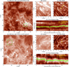 |
Fig. 1. Observation and analysis of oscillation events 1 and 5. The upper four panels (A–D) correspond to event 1 (starting from 05:14 UT on 2013 September 24). (A) The original IRIS SJ 1400 Å image showing the NOAA Active Region 11850. (B) Closer look at the region of interest, which is marked by a green box in (A). The cutout image processed by the MGN method is shown in (C). (D) Time–distance map constructed along the slit marked with a yellow line in (C). The distance starts at the bottom left of the slit indicated by a diamond symbol. In (D), the green triangles mark the position of the loop centre, and the yellow curve shows the fit result. The fitted displacement amplitude (A) and period (P) are indicated in the upper right corner. The lower four panels (E–H) are similar but correspond to event 5 (starting from 19:09UT on 2013 October 25). |
The oscillation parameters for these two examples, as well as the other five cases, are summarised in Table 1. All the events oscillate for more than three cycles without any apparent damping. For the case shown in Fig. 1D, the displacement amplitude even demonstrates a slight increase over time. The oscillation period ranges from 3 to 5 min, which is similar to that found in coronal bright points (Gao et al. 2022). Most TR loops have lengths falling in the range reported previously (1.2–20 Mm; see Hansteen et al. 2014; Brooks et al. 2016; Huang 2018; Huang et al. 2019). The displacement amplitudes are small, ranging from 0.036 to 0.098 Mm (∼0.3–0.8 pixels). However, previous studies have demonstrated the capability of such oscillation analysis techniques to provide measurements of subpixel amplitudes (e.g. see Sect. 4.3 in Gao et al. 2022). For comparison, the amplitudes of decayless oscillations in short coronal magnetic loops are 0.03–0.50 Mm (e.g. Gao et al. 2022; Petrova et al. 2023; Li & Long 2023; Shrivastav et al. 2023; Zhong et al. 2023a). We note that these studies are based on imaging observations with pixel sizes of 0.12–0.44 Mm, which have a spatial resolution approximately equal to or lower than that used in the present study.
Traditionally, decayless oscillations are interpreted as the fundamental kink standing waves, which are supported by the linear correlation between loop length and period (e.g. Anfinogentov et al. 2015; Li & Long 2023; Zhong et al. 2023a). Although there are several studies reporting the existence of higher harmonics in decayless oscillations (Duckenfield et al. 2018; Zhong et al. 2023b), the fundamental mode is most commonly detected and always has the most dominant power (e.g. see, Anfinogentov et al. 2015; Afanasyev et al. 2020; Karampelas & Van Doorsselaere 2020). Therefore, in the present study, we assume that the oscillations in TR loops correspond to the fundamental mode. In Fig. 2A, we present a scatter plot illustrating the relationship between oscillation period and loop length for decayless oscillation events both in our study and previous literature (Anfinogentov et al. 2013, 2015; Duckenfield et al. 2018; Zhong et al. 2022; Gao et al. 2022; Li & Long 2023; Mandal et al. 2022; Petrova et al. 2023; Shrivastav et al. 2023). There seem to be two different branches. For oscillations in longer loops, we still note a linear scaling. In particular, using the scatter points with a loop length of greater than 50 Mm, we calculate a Pearson correlation coefficient of 0.76, and show the linear fit result with the red solid line. However, for oscillations occurring in short loops (L < 50 Mm), we only obtain a correlation coefficient of 0.49. This means that there is no significant correlation between period and loop length. The decayless oscillations in the TR loops examined in this study fall within this branch. In Sect. 4.1, we provide a possible explanation for these two branches.
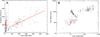 |
Fig. 2. Relationship between different oscillation parameters. (A) Scatter plot between the oscillation period and loop length for the oscillation events in our study (marked by red circles) and previous literature (Anfinogentov et al. 2013, 2015; Duckenfield et al. 2018; Zhong et al. 2022; Gao et al. 2022; Li & Long 2023; Mandal et al. 2022; Petrova et al. 2023; Shrivastav et al. 2023, marked by grey circles). The blue dashed line corresponds to a loop length of 50 Mm; the scatter points to its right are linearly fitted, with the best fit shown with the red solid line. (B) Scatter plot between the kink speed and loop length for the same data set, presented in log-log space for better visualisation. |
The energy flux F carried by these oscillations is also worth investigating. We can calculate F with the equation given in, for example, Van Doorsselaere et al. (2014) and Lim et al. (2023):
 (1)
(1)
The filling factor f and density ρ are assumed to be 10% (e.g. Van Doorsselaere et al. 2014; Lim et al. 2023; Guo et al. 2023) and 10−10 kg m−3 (consistent with the density measured in Sect. 4.2), respectively. Based on these values, the estimated average energy flux is ∼1.5 W m−2. Even when considering the recent study that suggests Eq. (1) requires modification by multiplying by a factor of ∼2 − 4 (as a result of Kelvin–Helmholtz instability development, as indicated by Guo et al. 2023), the energy flux of these oscillations is still insufficient to heat the transition region. This is not surprising as these TR loop oscillations are not commonly detected, which is associated with the highly dynamic behaviour and short lifetime of TR loops. Some energy-release events associated with magnetic reconnection could play a more significant role in heating the transition region (e.g. see Huang et al. 2015; Huang 2018; Pereira et al. 2018; Hou et al. 2021).
We also note that from the SJ image sequences, one or two TR loops seem to experience some overlapping with other structures at certain times, which raises the question of whether these loops maintain their identities throughout the entire duration. After checking the movies for all seven cases, we find that most of them remain stable enough to be regarded as individual loops. Also, all the events exhibit a “continuous” bright loop structure in TD maps, as shown in Figs. 1D and H. Therefore, we conclude that at least some of the TR loops presented in Table 1, if not all of them, indeed experience transverse oscillations.
4. Discussion
4.1. Interpreting the relationship between oscillation period and loop length
The result shown in Fig. 2A could be explained by the dependence of Alfvén speed on height in the upper solar atmosphere, as suggested in Gao et al. (2022). At greater heights, the corona tends to be globally stable, which leads to a relatively constant Alfvén speed across various locations and over different time intervals. The phase speed of the fundamental kink oscillation, that is, the kink speed ck = 2L/P in the long-wavelength limit, is close to the Alfvén speed. Therefore, for longer loops, L and P have a near-linear dependence. Using the linear fitting function corresponding to the red line in Fig. 2A, an average ck of (2.47 ± 0.21)×103 km s−1 can be estimated. The scattering of data points can be attributed to the fluctuations in the kink speed and the uncertainties in loop length measurements (see Anfinogentov et al. 2015).
On the other hand, shorter loops mainly distribute in the lower corona (or even in the TR), where physical properties such as density have more significant spatial variations. Also, there may be larger errors when estimating their loop lengths. The variation of the phase speed with loop length is further illustrated in Fig. 2B. We can see that ck spans a range of two orders of magnitude, and increases with the loop length or height (with a correlation coefficient of 0.87 in log–log space). Such a height dependence could be related to the decrease in density, assuming that the magnetic field strength does not change significantly with height. This is also consistent with the well-known fact that Alfvén speed in the solar atmosphere increases with height, ranging from ∼10 km s−1 in the photosphere to ∼1000 km s−1 in the corona (e.g. see Fig. 2 in Morton et al. 2023).
As for the oscillation events in our study (highlighted with red circles in Fig. 2), they fall within the “shorter loop” branch and have longer periods than what would be expected based on linear fitting from oscillation events in longer loops. Additionally, their phase speeds show an obvious increase with loop length. Considering the larger density gradient in the transition region, such a behaviour can be expected.
It is worth noting that we cannot rule out some other possibilities that may contribute to the relationship between P and L for shorter loops. The oscillations might be driven by photospheric p-modes (e.g. Riedl et al. 2019; Skirvin et al. 2023; Gao et al. 2023) or be associated with slow mode oscillations (see Lopin & Nagorny 2023).
4.2. TR seismology
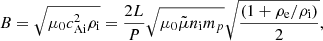
From the kink speed of these decayless oscillations in TR loops, we can roughly measure the magnetic field strength using the well-established seismology techniques (e.g. Tian et al. 2012; Nisticò et al. 2013; Anfinogentov & Nakariakov 2019; Gao et al. 2022; Li & Long 2023; Shrivastav et al. 2023; Zhong et al. 2023a). The Alfvén speed inside and outside of the loop can be expressed as  and
and 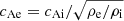 , where ρi (ρe) is the internal (external) density (e.g. Nakariakov & Ofman 2001; Anfinogentov & Nakariakov 2019; Zhong et al. 2023a). The average magnetic field strength of the loop can then be estimated as
 (2)
(2)
where μ0 is the magnetic permeability,  is the average molecular weight (can be taken as ∼1.27; e.g. Nisticò et al. 2013), ni is the internal number density, and mp is the proton mass. We use the intensity ratio of O IV 1400/1401 Å doublets (e.g. Tian et al. 2014) to determine ni (see Fig. 3). The density diagnosis is performed for events 1 and 5 shown in Fig. 1. In the TD maps (Figs. 1D and H), we note that the IRIS spectrograph slit has scanned across the oscillating loop. The spectral profiles near O IV lines can be seen in Figs. 3A and B. We use a multi-Gaussian fit to obtain the line intensities, which are then used to estimate the densities based on the theoretically predicted curve (shown in Fig. 3C) of O IV line ratios and number densities obtained from the CHIANTI database (Dere et al. 1997; Del Zanna et al. 2021). The density values for these two events are
 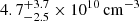 and
and 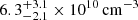 . The signal-to-noise ratio (S/N) for event 5 (Fig. 3B) is higher than that for event 1 (Fig. 3A), resulting in a smaller error. Such density values are comparable to the results of previous studies (e.g. Brooks et al. 2016; Huang 2018; Huang et al. 2019). The density outside the loop is not easy to measure with such a method due to a low S/N, and so we simply take the density ratio ρe/ρi to be 1/3 (see Li & Long 2023; Petrova et al. 2023; Shrivastav et al. 2023). Now using Eq. (1), the magnetic field can be estimated as
  G and
G and  G. These values are lower than the TR magnetic field strengths proposed or measured in some previous studies (e.g. Huang et al. 2019; Ishikawa et al. 2021; Gupta & Nayak 2022). However, as indicated by Berghmans et al. (2021) and Shrivastav et al. (2023), the loop length can be underestimated by 40–50%, which could result in significant underestimation of B based on Eq. (2). In the future, we hope to be able to measure the loop length and magnetic field more accurately using high-resolution photospheric magnetograms to determine the footpoints of TR loops.
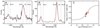 |
Fig. 3. Density diagnosis for events 1 and 5. (A) and (B) IRIS spectral profiles (black lines), including the O IV 1400/1401 doublet lines used for the density diagnosis. Panel (A) corresponds to event 1 shown in Figs. 1A–D, while (B) corresponds to event 5 shown in Figs. 1E–H. The red dashed lines are the multi-Gaussian fitting result. (C) Theoretically predicted curve associating the O IV intensity ratio with the electron number density. The small black and red squares represent the intensity ratios obtained from (A) and (B), respectively, as well as their corresponding densities. The error bars are also added. |
In conclusion, the newly detected decayless kink oscillations shed light on a novel approach to diagnosing the TR magnetic field, namely TR seismology. However, this approach is limited by the difficulties in identifying kink oscillations in TR loops, as well as the potentially large uncertainties related to the error in estimating the loop length and density.
5. Summary
This study presents the identification of seven decayless transverse oscillation events in TR loops with their properties listed in Table 1. To the best of our knowledge, it is the first time that such oscillations are detected in the TR. The TR loops studied here have short lengths, ranging from 9 to 26 Mm. The oscillation periods and displacement amplitudes are 3–5 min and 0.037–0.098 Mm, respectively. Assuming that these oscillations are fundamental kink standing waves, we can obtain a kink speed of 60–280 km s−1. In addition, the kink speed clearly increases with loop length. Along with the density derived from the O IV line ratios, we can also provide a rough estimate of the average magnetic field along the TR loop.
For future works, we plan to perform an MHD simulation and forward modelling to achieve a better understanding of these oscillations. It is also important to identify more oscillation events in observations in order to investigate their excitation mechanism and make comparisons between the decayless oscillations in the TR loops and those in the coronal loops.
Acknowledgments
This work is supported by National Key R&D Program of China No. 2021YFA1600500 and NSFC grant 12303057. Y.G. is supported by China Scholarship Council under file No. 202206010018. T.V.D. is supported by the C1 grant TRACEspace of Internal Funds KU Leuven, and a Senior Research Project (G088021N) of the FWO Vlaanderen. M.G. acknowledges support from the National Natural Science Foundation of China (NSFC, 12203030). The research benefited greatly from discussions at ISSI. IRIS is a NASA small explorer mission developed and operated by LMSAL with mission operations executed at the NASA Ames Research Center and major contributions to downlink communications funded by ESA and the Norwegian Space Centre. CHIANTI is a collaborative project involving George Mason University, the University of Michigan (USA), and the University of Cambridge (UK). We would like to thank Yajie Chen, Zhenghua Huang, and Daye Lim for their helpful comments and suggestions.
References
- Afanasyev, A. N., Van Doorsselaere, T., & Nakariakov, V. M. 2020, A&A, 633, L8 [NASA ADS] [CrossRef] [EDP Sciences] [Google Scholar]
- Anfinogentov, S. A., & Nakariakov, V. M. 2019, ApJ, 884, L40 [CrossRef] [Google Scholar]
- Anfinogentov, S., Nisticò, G., & Nakariakov, V. M. 2013, A&A, 560, A107 [NASA ADS] [CrossRef] [EDP Sciences] [Google Scholar]
- Anfinogentov, S. A., Nakariakov, V. M., & Nisticò, G. 2015, A&A, 583, A136 [NASA ADS] [CrossRef] [EDP Sciences] [Google Scholar]
- Berghmans, D., Auchère, F., Long, D. M., et al. 2021, A&A, 656, L4 [NASA ADS] [CrossRef] [EDP Sciences] [Google Scholar]
- Brooks, D. H., Reep, J. W., & Warren, H. P. 2016, ApJ, 826, L18 [NASA ADS] [CrossRef] [Google Scholar]
- De Pontieu, B., Title, A. M., Lemen, J. R., et al. 2014, Sol. Phys., 289, 2733 [Google Scholar]
- Del Zanna, G., Dere, K. P., Young, P. R., & Landi, E. 2021, ApJ, 909, 38 [NASA ADS] [CrossRef] [Google Scholar]
- Dere, K. P., Landi, E., Mason, H. E., Monsignori Fossi, B. C., & Young, P. R. 1997, A&AS, 125, 149 [NASA ADS] [CrossRef] [EDP Sciences] [Google Scholar]
- Duckenfield, T., Anfinogentov, S. A., Pascoe, D. J., & Nakariakov, V. M. 2018, ApJ, 854, L5 [Google Scholar]
- Gao, Y., Tian, H., Van Doorsselaere, T., & Chen, Y. 2022, ApJ, 930, 55 [NASA ADS] [CrossRef] [Google Scholar]
- Gao, Y., Guo, M., Van Doorsselaere, T., Tian, H., & Skirvin, S. J. 2023, ApJ, 955, 73 [NASA ADS] [CrossRef] [Google Scholar]
- Guo, M., Gao, Y., Van Doorsselaere, T., & Goossens, M. 2023, A&A, 676, L7 [NASA ADS] [CrossRef] [EDP Sciences] [Google Scholar]
- Gupta, G. R., & Nayak, S. S. 2022, MNRAS, 512, 3149 [CrossRef] [Google Scholar]
- Hansteen, V., De Pontieu, B., Carlsson, M., et al. 2014, Science, 346, 1255757 [Google Scholar]
- Hou, Z., Huang, Z., Xia, L., et al. 2021, Symmetry, 13, 1390 [NASA ADS] [CrossRef] [Google Scholar]
- Huang, Z. 2018, ApJ, 869, 175 [NASA ADS] [CrossRef] [Google Scholar]
- Huang, Z., Xia, L., Li, B., & Madjarska, M. S. 2015, ApJ, 810, 46 [NASA ADS] [CrossRef] [Google Scholar]
- Huang, Z., Li, B., Xia, L., et al. 2019, ApJ, 887, 221 [NASA ADS] [CrossRef] [Google Scholar]
- Ishikawa, R., Trujillo Bueno, J., del Pino Alemán, T., et al. 2021, Sci. Adv., 7, eabe8406 [NASA ADS] [CrossRef] [Google Scholar]
- Karampelas, K., & Van Doorsselaere, T. 2020, ApJ, 897, L35 [Google Scholar]
- Li, D., & Long, D. M. 2023, ApJ, 944, 8 [NASA ADS] [CrossRef] [Google Scholar]
- Li, D., Bai, X., Tian, H., et al. 2023, A&A, 675, A169 [NASA ADS] [CrossRef] [EDP Sciences] [Google Scholar]
- Lim, D., Van Doorsselaere, T., Berghmans, D., et al. 2023, ApJ, 952, L15 [NASA ADS] [CrossRef] [Google Scholar]
- Lopin, I., & Nagorny, I. 2023, MNRAS, 519, 5579 [NASA ADS] [CrossRef] [Google Scholar]
- Mandal, S., Chitta, L. P., Antolin, P., et al. 2022, A&A, 666, L2 [NASA ADS] [CrossRef] [EDP Sciences] [Google Scholar]
- Morgan, H., & Druckmüller, M. 2014, Sol. Phys., 289, 2945 [Google Scholar]
- Morton, R. J., Sharma, R., Tajfirouze, E., & Miriyala, H. 2023, Rev. Mod. Plasma Phys., 7, 17 [NASA ADS] [CrossRef] [Google Scholar]
- Nakariakov, V. M., & Ofman, L. 2001, A&A, 372, L53 [NASA ADS] [CrossRef] [EDP Sciences] [Google Scholar]
- Nakariakov, V. M., Anfinogentov, S. A., Nisticò, G., & Lee, D. H. 2016, A&A, 591, L5 [NASA ADS] [CrossRef] [EDP Sciences] [Google Scholar]
- Nisticò, G., Nakariakov, V. M., & Verwichte, E. 2013, A&A, 552, A57 [NASA ADS] [CrossRef] [EDP Sciences] [Google Scholar]
- Pereira, T. M. D., Rouppe van der Voort, L., Hansteen, V. H., & De Pontieu, B. 2018, A&A, 611, L6 [NASA ADS] [CrossRef] [EDP Sciences] [Google Scholar]
- Petrova, E., Magyar, N., Van Doorsselaere, T., & Berghmans, D. 2023, ApJ, 946, 36 [CrossRef] [Google Scholar]
- Riedl, J. M., Van Doorsselaere, T., & Santamaria, I. C. 2019, A&A, 625, A144 [NASA ADS] [CrossRef] [EDP Sciences] [Google Scholar]
- Shrivastav, A. K., Pant, V., Berghmans, D., et al. 2023, A&A, submitted [arXiv:2304.13554] [Google Scholar]
- Skirvin, S. J., Gao, Y., & Van Doorsselaere, T. 2023, ApJ, 949, 38 [NASA ADS] [CrossRef] [Google Scholar]
- Tian, H., McIntosh, S. W., Wang, T., et al. 2012, ApJ, 759, 144 [Google Scholar]
- Tian, H., DeLuca, E., Reeves, K. K., et al. 2014, ApJ, 786, 137 [NASA ADS] [CrossRef] [Google Scholar]
- Tomczyk, S., Card, G. L., Darnell, T., et al. 2008, Sol. Phys., 247, 411 [Google Scholar]
- Van Doorsselaere, T., Gijsen, S. E., Andries, J., & Verth, G. 2014, ApJ, 795, 18 [NASA ADS] [CrossRef] [Google Scholar]
- Van Doorsselaere, T., Srivastava, A. K., Antolin, P., et al. 2020, Space Sci. Rev., 216, 140 [Google Scholar]
- Wang, T., Ofman, L., Davila, J. M., & Su, Y. 2012, ApJ, 751, L27 [Google Scholar]
- Yang, Z., Tian, H., Tomczyk, S., et al. 2020a, Sci. China E Technol. Sci., 63, 2357 [CrossRef] [Google Scholar]
- Yang, Z., Bethge, C., Tian, H., et al. 2020b, Science, 369, 694 [Google Scholar]
- Zhong, S., Nakariakov, V. M., Kolotkov, D. Y., Verbeeck, C., & Berghmans, D. 2022, MNRAS, 516, 5989 [NASA ADS] [CrossRef] [Google Scholar]
- Zhong, S., Nakariakov, V. M., Miao, Y., Fu, L., & Yuan, D. 2023a, Sci. Rep., 13, 12963 [NASA ADS] [CrossRef] [Google Scholar]
- Zhong, S., Nakariakov, V. M., Kolotkov, D. Y., et al. 2023b, Nat. Commun., 14, 5298 [NASA ADS] [CrossRef] [Google Scholar]
All Tables
All Figures
|
Fig. 1. Observation and analysis of oscillation events 1 and 5. The upper four panels (A–D) correspond to event 1 (starting from 05:14 UT on 2013 September 24). (A) The original IRIS SJ 1400 Å image showing the NOAA Active Region 11850. (B) Closer look at the region of interest, which is marked by a green box in (A). The cutout image processed by the MGN method is shown in (C). (D) Time–distance map constructed along the slit marked with a yellow line in (C). The distance starts at the bottom left of the slit indicated by a diamond symbol. In (D), the green triangles mark the position of the loop centre, and the yellow curve shows the fit result. The fitted displacement amplitude (A) and period (P) are indicated in the upper right corner. The lower four panels (E–H) are similar but correspond to event 5 (starting from 19:09UT on 2013 October 25). |
| In the text | |
|
Fig. 2. Relationship between different oscillation parameters. (A) Scatter plot between the oscillation period and loop length for the oscillation events in our study (marked by red circles) and previous literature (Anfinogentov et al. 2013, 2015; Duckenfield et al. 2018; Zhong et al. 2022; Gao et al. 2022; Li & Long 2023; Mandal et al. 2022; Petrova et al. 2023; Shrivastav et al. 2023, marked by grey circles). The blue dashed line corresponds to a loop length of 50 Mm; the scatter points to its right are linearly fitted, with the best fit shown with the red solid line. (B) Scatter plot between the kink speed and loop length for the same data set, presented in log-log space for better visualisation. |
| In the text | |
|
Fig. 3. Density diagnosis for events 1 and 5. (A) and (B) IRIS spectral profiles (black lines), including the O IV 1400/1401 doublet lines used for the density diagnosis. Panel (A) corresponds to event 1 shown in Figs. 1A–D, while (B) corresponds to event 5 shown in Figs. 1E–H. The red dashed lines are the multi-Gaussian fitting result. (C) Theoretically predicted curve associating the O IV intensity ratio with the electron number density. The small black and red squares represent the intensity ratios obtained from (A) and (B), respectively, as well as their corresponding densities. The error bars are also added. |
| In the text | |
Current usage metrics show cumulative count of Article Views (full-text article views including HTML views, PDF and ePub downloads, according to the available data) and Abstracts Views on Vision4Press platform.
Data correspond to usage on the plateform after 2015. The current usage metrics is available 48-96 hours after online publication and is updated daily on week days.
Initial download of the metrics may take a while.