| Issue |
A&A
Volume 681, January 2024
|
|
|---|---|---|
| Article Number | A23 | |
| Number of page(s) | 29 | |
| Section | Planets and planetary systems | |
| DOI | https://doi.org/10.1051/0004-6361/202347670 | |
| Published online | 03 January 2024 | |
Debiased population of very young asteroid families
1
Institute of Astronomy, Charles University,
V Holešovičkách 2,
180 00
Prague 8,
Czech Republic
e-mail: This email address is being protected from spambots. You need JavaScript enabled to view it.
2
Department of Space Studies, Southwest Research Institute,
1050 Walnut St., Suite 300,
Boulder,
CO
80302,
USA
Received:
7
August
2023
Accepted:
20
October
2023
Abstract
Context. Asteroid families that are less than one million years old offer a unique possibility to investigate recent asteroid disruption events and test ideas about their dynamical evolution. Observations provided by powerful all-sky surveys have led to an enormous increase in the number of detected asteroids over the past decade. When the known populations are well characterized, they can be used to determine asteroid detection probabilities, including those in young families, as a function of their absolute magnitude.
Aims. We use observations from the Catalina Sky Survey (CSS) to determine the bias-corrected population of small members in four young families down to sizes equivalent to several hundred meters.
Methods. Using the most recent catalog of known asteroids, we identified members from four young families for which the population has grown appreciably over recent times. A large fraction of these bodies have also been detected by CSS. We used synthetic populations of asteroids, with their magnitude distribution controlled by a small number of parameters, as a template for the bias-corrected model of these families. Applying the known detection probability of the CSS observations, we could adjust these model parameters to match the observed (biased) populations in the young families.
Results. In the case of three families, Datura, Adelaide, and Rampo, we find evidence that the magnitude distribution transitions from steep to shallow slopes near 300 to 400 meters. Conversely, the Hobson family population may be represented by a single power-law model. The Lucascavin family has a limited population; no new members have been discovered over the past two decades. We consider a model of parent body rotational fission with the escaping secondary tidally split into two components (thereby providing three members within this family). In support of this idea, we find that no other asteroid with absolute magnitude H ≤ 18.3 accompanies the known three members in the Lucascavin family. A similar result is found for the archetypal asteroid pair Rheinland–Kurpfalz.
Key words: celestial mechanics / minor planets, asteroids: general
© The Authors 2024
 Open Access article, published by EDP Sciences, under the terms of the Creative Commons Attribution License (https://creativecommons.org/licenses/by/4.0), which permits unrestricted use, distribution, and reproduction in any medium, provided the original work is properly cited.
This article is published in open access under the Subscribe to Open model. This email address is being protected from spambots. You need JavaScript enabled to view it. to support open access publication.
1 Introduction
More than a century ago, Hirayama (1918) discovered the first examples of statistically significant clusters in the space of asteroid heliocentric orbital elements (using proper values of the semimajor axis, eccentricity, and inclination). Suspecting their mutual relation, he coined the term asteroid families. Hirayama rightly proposed that the families are collections of asteroids related to parent bodies that disrupted sometime in the past. He even identified asteroid collisions as the source of these catastrophic events. Over time, asteroid families became a core element of Solar System small body science. They provide (i) an important constraint on asteroid collisional models; (ii) a unique tool to study the internal structure of large asteroids, both in terms of their chemical homogeneity and mechanical structure; (iii) an important source of impactor showers that include both large projectiles and dust onto the surfaces of the terrestrial planets (including the Earth); (iv) an arena for studying a plethora of dynamical processes affecting the orbits and spins of asteroids; and (v) many more (see, e.g., recent reviews by Nesvorný et al. 2015; Masiero et al. 2015; Michel et al. 2015; Novaković et al. 2022).
In this paper, we explore (ii), namely the capability of asteroid family data to constrain the internal structure of the parent body. Over the past two decades or so, sophisticated numerical approaches have been developed to model energetic asteroidal collisions, the subsequent dispersal, and gravitational re-accumulation of resulting fragments (e.g., Michel et al. 2015; Asphaug et al. 2015; Jutzi et al. 2015). The outcome of these simulations, which may be compared to the information provided by asteroid families, sensitively depends on assumptions about the internal properties of the parent body. One type of dataset includes the size frequency distribution of asteroid members in the family. While determining asteroid family members looks straightforward, it has potential complications. This is because many families extend over non-negligible portions of the asteroid belt. As a result, the proper zone in orbital element space in which the family members are located may contain a certain fraction of unrelated (interloping) asteroids. Methods to estimate the interloper fraction have been developed (e.g., Migliorini et al. 1995), but their validity is limited and their results are necessarily of a statistical, rather than deterministic, nature. Additionally, progress from powerful and automated surveys over the past decades makes it more difficult to deal with the interloper problem because small asteroid spatial densities increasely fill proper element space. Unless we know the size distribution of the background and the family population, more asteroids mean that there are more interlopers to deal with.
Fortunately, the ability of surveys to increase the known asteroid populations has also brought into play a new and interesting niche that allows us to determine the complete (bias-corrected) population of the family members. The fundamental goal of this paper is to try to exploit this possibility. Our focus here is on a special subclass of asteroid families characterized by extremely young ages, namely those that are ≃1 Myr or less. Already the first examples, which were discovered little less than two decades ago (Nesvorný et al. 2006; Nesvorný & Vokrouhlický 2006), help us understand the means to get rid of potential interlopers. Consider that the unusual youth of these families means that five of the six osculating orbital elements are clustered (semimajor axis a, eccentricity e, inclination I, and longitudes of node Ω and perihelion ϖ), rather than the standard three proper orbital elements used for most family work (semimajor axis ap, eccentricity ep, and inclination Ip). This immediately has two positive consequences. First, our work can use simpler osculating elements rather than less (population-wise) accessible proper elements. Second, the additional two dimensions of the orbital element arena in which we searched for these very young families have a diluted spatial density of known asteroids. The very young families show up as distinct, and often isolated clusters, allowing us to largely circumvent the interloper problem. Additionally, their recent origin has allowed us to accurately determine each family’s age by propagating the asteroid orbits backward in time and then by observing how the orbits rearrange themselves into a tighter cluster at the epoch of its formation. This procedure has helped to further eliminate interlopers.
As far as the population count is concerned, we are then left with the observational bias produced by telescopic limitations (basically the capability of a given instrument to detect asteroids to some apparent magnitude). Here we can compensate for this problem to a degree by using asteroids taken from a well-characterized and sufficiently long-lasting survey. Profiting from our earlier work, in which we developed a new model for the near-Earth asteroid population, we use a careful characterization of the Catalina Sky Survey (1.5-m Mt. Lemmon telescope, G96) observations in between 2016 and 2022. We apply this rich dataset to determine the bias-corrected population of four very young families and a few more clusters of interest1.
We first briefly describe the observation set in Sect. 2. Next, we introduce the very young families that we are going to analyze in this paper (Sect. 3), providing their new identification and full membership in the Appendix. In Sect. 4, we develop an approach to determine the complete population of the families, based on their biased population and information about the survey detection probability, and we apply it to the selected cases. In Sect. 5, we discuss the implications of our results and provide some discussion of potential future work.
2 Catalina Sky Survey observations
Catalina Sky Survey2 (CSS), managed by Lunar and Planetary Laboratory of the University of Arizona, has been one of the most prolific survey programs over the past decade (e.g., Christensen et al. 2019). While primarily dedicated to the discovery and further tracking of near-Earth objects with the goal to characterize a significant fraction of the population with sizes as small as 140 m, CSS observations represent an invaluable source of information for other studies in planetary science or astronomy in general.
Here, we use observations of the CSS 1.5-m survey telescope located at Mt. Lemmon (MPC observatory code G96). Our method builds on the work of Nesvorný et al. (2023), who constructed a new model of the near-Earth object population using CSS data. They carried out a detailed analysis of the asteroid detection probabilities for the G96 operations over the period between January 2013 and June 2022. This interval was divided into two phases: (i) observations before May 14, 2016 (phase 1), and (ii) observations after May 31, 2016 (phase 2). The first phase contained 61 585 well-characterized frames, in the form of sequences of four that were typically 30 s exposure images, while the second phase had 162 280 well-characterized frames. The reason for the difference was due to longer timespan of the phase 2 but also an important upgrade of the CSS CCD camera in the second half of May 2016. The new camera had four times the field of view, and better photometric sensitivity, allowing the survey to cover a much larger latitude region about the ecliptic. The superiority of the CSS observations taken during phase 2 allows us to drop the phase 1 data in most of the work below. Only in the case of Lucascavin family and Rheinland-Kurpfalz pair do we combine observations from the two phases into a final result.
The final product of interest for our work here is the detection probability p(H) as a function of the absolute magnitude H for asteroids in a chosen family. In principle, p depends not only on H, but on all orbital elements (in other words, it is specific to a particular body). Members in the youngest known asteroid families to date, however, have their orbit longitudes A uniformly distributed in between 0° and 360°. This is because the characteristic λ dispersal timescale after the family forming event is only about 1–3 kyr; all families which we consider here are at least an order of magnitude older than this value. Conversely, a property of very young asteroid families are that they have a tight clustering in the other five orbital elements, including the longitude of node Ω and longitude of perihelion ϖ. As a result, the detection probability p(H) assigned to a given family has been computed using the mean values of osculating orbital elements, except for λ where the individual probabilities have been averaged3. Only in the case of two families – Datura and Rampo – we used the secular angles Ω and ϖ to randomly sample their observed interval of values shown in Figs. 1 and 9. As seen in those figures, and expected from theoretical considerations, the Ω vs. ϖ values are strongly correlated in very young families. We take this correlation into account when computing the mean detection probability p(H).
Apart from p(H), we can also determine a detection rate r(H), namely a statistically mean number of the survey fields of view in which a given family member with an absolute magnitude H should have been detected. While correlated with p(H), r(H) contains additional information and may be thus used as a consistency check in our analysis below. Technical details of the numerical methods that allow us to determine p(H) and r(H) can be found in Nesvorný et al. (2023).
3 Very young families
In this section we introduce four very young asteroid families, namely Datura, Adelaide, Hobson and Rampo, whose known population is large enough that they are suitable candidates for our debiasing efforts4. We also consider two additional families, Wasserburg and Martes, that have extremely young ages but whose population is limited. For these examples, we do not perform a full-scale debiasing analysis but instead argue that a large population of small undetected members should exist near the currently known population. Finally, we consider two special cases: the very young asteroid family Lucascavin and the asteroid pair Rheinland–Kurpfalz. Here, our goal is actually opposite to the previous cases. Our working hypothesis is that further smaller fragments in their location might not exist. As a result, we use CSS observations to set an upper limit on the size or magnitude of the unseen members to explore whether this hypothesis might be correct.
Table 1 provides a basic overview of the asteroid clusters and pairs that are analyzed in this paper, as well as some notes on the goals we hope to achieve. The identification method used to find the families, and full listing of the family members for each family analyzed in this paper, is provided in the Appendix. In what follows, we provide basic information about the investigated families, with slightly more attention paid to the Datura family. The debiasing procedure to constrain a complete population of members in the above-mentioned families is presented in the next Sect. 4.
Asteroid families and pairs studied in this paper.
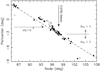 |
Fig. 1 Osculating values of the secular angles – longitude of node Ω (abscissa) and longitude of perihelion ϖ (ordinate) – for members in the Datura family (epoch MJD 60 000.0). The black symbols show multi-opposition orbits, gray symbols are for the singleopposition orbits; diamond symbol for (1270) Datura, the largest member. Larger/smaller relative values of the secular angles, measured with respect to (1270) Datura, are correlated with positive/negative shift in proper semimajor axis ∆aP (as explained by the arrows). Because the node drifts in a retrograde sense, while the perihelion drifts in the prograde sense, their trends are opposite to each other (thence anticorrelation of the two angles). Location of the exterior mean motion resonance M9/16 with Mars is mapped where the label shows. The dashed line with a slope −0.5 indicates the (anti-) correlation trend. The symbol indicated by a question mark shows projection of (429988) 2013 PZ36 (an object captured on a very chaotic orbit possibly in the exterior mean motion resonance E3/10 with Earth), whose association to the Datura family is uncertain. |
3.1 Very young families with large population of members
Datura. The cluster of asteroids about the largest member (1270) Datura is an archetype of very young families. In this sense it is comparable to the Karin family, which is an excellent example of a sizable young family having an age less than ≃10 Myr but secular angles distributed uniformly in the 0° to 360° interval. Not only is the Datura family the first example discovered in the very young family class (Nesvorný et al. 2006, see also Nesvorný & Vokrouhlický 2006), but its location in the inner part of the main belt allowed us to readily collect the physical parameters of the largest members and study the role of the very young families in a broader context of planetary science (e.g., Mothé-Diniz & Nesvorný 2008; Vernazza et al. 2009; Vokrouhlický et al. 2008, 2009, 2017a). The number of known members in the Datura family has also grown quickly from only 7 in 2006 to 17 in 2017.
Here we make use of the accelerating pace with which asteroids have been discovered during recent years and report a currently known Datura population of Nobs = 91 members (possibly even 94 members, see Table A.1). Importantly, NCSS = 60 of them has been also detected by CSS during its phase 2 operations. We note that Vokrouhlický et al. (2017a) already attempted to use CSS observations for their Datura population debiasing efforts. Our current work, however, surpasses the detail and accuracy of this earlier work. Vokrouhlický et al. (2017a) could use only the 13 largest members in the Datura family detected by CSS between 2005 and 2012. Thanks to the camera update by CSS in 2016, the six years of CSS operations between 2016 and 2022 has led to a much larger Datura population and an improved characterization of family member detection probabilities.
Before we turn our attention to the magnitude distribution of the Datura members, we use this family to exemplify some common features of very young clusters. They help to justify membership of given asteroids within the family, even without a further substantiation via a detailed study of their past orbital convergence using numerical integrations (see a brief discussion of this issue in the Appendix). A correlation between the osculating values of the secular angles, namely longitude of node Ω and longitude of perihelion ϖ, is a characteristic property of several very young families (unless the family is extremely young, such that Ω and ϖ are clustered within a degree or so, basically corresponding to their initial dispersal). Denoting ∆Ω and ∆ϖ as the angular difference with respect to the largest body in the family, the initial phase of the dispersal process is described by a linear approximation. Thus at time T, one has ∆Ω(T) ≃ CT + O(T2) and a similar equation for the longitude of perihelion, with C = (∂s/∂a) ∆a, where s is the proper nodal frequency and ∆a is the difference in semimajor axis with respect to the largest body produced by the initial velocity ejection. The smallest observed fragments in Datura have ∆a ≃ 2 × 10⁻³ au, corresponding to their ejection by ≃10 m s−1 (only slightly larger than the escape velocity from the parent body of the family). Together with (∂s/∂a) ≃ 40 arcsec yr−1 au−1, we can estimate their angular difference ∆Ω ≃ 11° in T ≃ 500 kyr (see Fig. 1). A similar analysis for ∆ϖ results in about half this value.
Given that in both ∆Ω and ∆ϖ the nonlinear terms in time T are still very small (those will be produced by the Yarkovsky drift in semimajor axis of the small members in the family; e.g., Vokrouhlický et al. 2009, 2017a), they are strongly correlated with a slope −0.5. The early dispersal phase of very young families is characterized by additional correlations between the osculating elements, namely (i) the eccentricity and longitude of perihelion, and (ii) the inclination and the longitude of node (see, e.g., data in the tables given in the Appendix). As mentioned above, these extra correlations between osculating orbital elements help to strengthen justification of the membership in the family.
The cumulative magnitude distribution N(< H) of Datura family members is shown in Fig. 2. The magnitudes H for the six lowest-numbered members were determined accurately using calibrated observations, and expressed at the mid-value of the lightcurve, by Vokrouhlický et al. (2009, 2017a). The magnitudes for other Datura members were taken from the MPC catalog. We show both the distribution of all known members (black symbols), and highlight also the sample of 60 members which have been detected by CSS (red symbols). Data for these asteroids may be used for debiasing of the Datura family population, since only for them we have the detection probability well characterized.
The bottom panel of Fig. 2 shows detection probability p(H) of Datura members as a function of their absolute magnitude. As explained above, this is a result based on an analysis of 10 000 synthetic orbits in the Datura family zone which makes p(H) very smooth. At the first sight, it might be surprising that p ≃ 1 up to magnitude 18, signaling that the population of the family members is complete up to that limit. This inference, however, is correct and a result of (i) a six year survey , (ii) the small value of Datura-like orbital inclinations, such that CSS fields-of-view did not miss an opportunity to detect the asteroids in the Datura family, and (iii) a typical 50% photometric detection limit of CSS in between 20.5 and 21.5 apparent magnitude (in the visual bands). Neglecting a small phase-angle correction in the Pogson’s relation between absolute H and apparent m magnitudes, we have H ≃ m − 5 log(r ∆), where r and ∆ are heliocentric and geocentric distances of the asteroid. At opposition, and near aphelion to cover the worst case situation, we have r ≃ 2.7 au and ∆ ≃ 1.7 au. As a result, the limiting magnitude m ≃ 21 translates to H ≃ 17.8. During the 6 yr period of CSS phase 2, the configuration eventually becomes favorable to detection, explaining the completion limit at H ≃ 18 magnitude. At the opposite end of things, the probability p has a tail to nearly 21 magnitude. This means CSS with its best nightly limits near the apparent 22 magnitude have a chance to detect small Datura members when they happen to be near the perihelion of their orbit at opposition.
In order to verify that the detection probability p(H) shown in Fig. 2 is reasonable, we also determined the expected mean rate r(H) of CSS phase 2 detections and compared it with the actual number of detections of all 60 identified Datura members. This result is presented in Fig. 3. The largest body (1270) Datura was found to be detected 18 times, and even members up to magnitude H = 18 were typically detected more than 10 times. This is a good verification of population completeness. Only after that limit does the number of detections decrease, with no Datura member having H > 20 magnitude detected. This outcome corresponds to the inferred detection probability: p < 0.1 for H > 20.
The mean value of the actual Datura-member detections computed using a running window of consecutive 7 asteroids is shown by the blue curve. The scatter of the number of detections about the predicted red line is not surprising because the latter has been computed as a mean value from 10 000 synthetic Datura members. The important point is that the blue curve, though computed as a mean over a much smaller number of cases (additionally having different H values), reasonably follows the predicted mean rate. This points to consistency in evaluation of the detection probability too.
Adelaide. The cluster of five small objects about the inner main belt asteroid (525) Adelaide was first reported by Novaković & Radović (2019). Apart from an approximate age of 500 kyr, few details were given in this paper. Carruba et al. (2020), while trying to search for secondary subclusters in the very young asteroid families, analyzed the Adelaide family and identified 19 of its members. The case was finally revisited by Vokrouhlický et al. (2021b), who noted a significant population increase to about 50 small asteroids in this family. They confirmed the earlier age estimate and considered a possibility of a causal link between formation of the Datura and Adelaide families (which they rejected). Novaković et al. (2022) identified already 72 members, and our current census of the Adelaide family population reveals Nobs = 79 members, yet another important increase. The population increase rate of the Adelaide family is among the largest of the very young families. A fortunate circumstance for our analysis is that NCSS = 63 of the members were also detected by CSS in its phase 2.
Figure 4 shows the osculating secular angles Ω and ϖ of the Adelaide family population from Table A.2. The Ω vs. ϖ correlation is weaker than that of the Datura-family members (Fig. 1). Vokrouhlický et al. (2021b), while analyzing behavior of the backward propagated orbits in the Adelaide family, noted a weak chaotic signature triggered by a conjoint effect of weak mean-motion resonances and distant encounters with Mars. We suspect they are also the origin of the observed scatter in the correlation between the secular angles seen in Fig. 4. Nevertheless, the orbits show a high degree of clustering even in the subspace of the secular angles, which in effect strengthens their membership in the family.
The cumulative magnitude distribution of the Adelaide members is shown in Fig. 5. Its extreme behavior has been already noted by Vokrouhlický et al. (2021b): (i) the largest remnant (525) Adelaide is separated from other members in the family by an unusually large gap of 6 magnitudes in the absolute magnitude H scale, and (ii) the small fragment population has an extremely steep H-distribution in between 18 and 19 (the local power-law N(< H) ∝ 10γH approximation requires γ ≃ 2 or even larger). This shape is characteristic of a cratering event on (525) Adelaide.
The bottom panel in Fig. 5 shows the mean detection probability p(H) of the Adelaide members. The range in which p(H) drops from one to zero, namely H ≃ 18.4 to H ≃ 20.4 magnitudes, is narrower than in the case of the Datura family (with the completion limit at even higher magnitude). This is readily explained by a smaller eccentricity of Adelaide-like orbits for nearly the same value of semimajor axis and inclination.
To further check our results, we also compared the number of CSS phase 2 detections of the 63 Adelaide members and their mean computed rate r(H) (Fig. 6). The largest asteroid (525) Adelaide has been detected 8 times, which conforms – within fluctuation – to the predicted rate of about 13. We note the decrease of r(H) for objects brighter than magnitude 13. This phenomenon in the CSS observations has to do with the saturation of the signal for bright objects, as they can become confused with stationary sources hiding their sky-plane motion. Such a configuration may occasionally happen when (525) Adelaide is at opposition near perihelion of its orbit. Small members then sample the tail of r(H) values with only few detections predicted. The running mean of detections (blue curve) appears to follow the predicted r(H) dependence reasonably well.
Hobson. Pravec & Vokrouhlický (2009) identified a small cluster of asteroids associated with the largest member (57738) 2001 UZ160 and set an upper age of 500 kyr for its formation event. They also noted a nearby asteroid (18777) Hobson, but were unsure about its relation to the cluster, mainly because Hobson and 2001 UZ160 have similar sizes, which they considered unusual for the outcome of a collisional fragmentation of the parent body. Rosaev & Plávalová (2016, 2017, 2018) then revisited the situation and proved that Hobson was associated with the cluster. They derived an age for the family of 365 ± 67 kyr. By 2018, their Hobson population consisted of nine members, which shortly improved to 11 by the work of Pravec et al. (2018). These latter authors also rejected the possibility of the Hobson family formation by rotation fission, and conducted valuable photometric observations of the two largest members Hobson and 2001 UZ160. The two similar-size largest remnants also intrigued Vokrouhlický et al. (2021a), who revisited the nature of the parent object of this family (counting already 45 Hobson members, and Novaković et al. (2022) reported another increase to 51 members). Using the SPH/N-body formation simulation, their results implied a very special impact and target combination was required. As a novel idea, they also argued the Hobson family may result from collisional fragmentation of a component in a parent binary. In this work we report Nobs = 60 members (likely even one more, see Table A.3), out of which NCSS = 33 were detected during the phase 2 of CSS operations.
The dispersion of the secular angles within about two degrees is a consequence of the very young age of the Hobson family. We thus turn our attention directly to the cumulative magnitude distribution of its members shown on Fig. 7. The two largest asteroids – (18777) Hobson and (57738) 2001 UZ160 – are its most outstanding feature. Their orbital convergence has been independently verified by Rosaev & Plávalová (2017, 2018) and Vokrouhlický et al. (2021a), while Pravec et al. (2018) determined the identical values of the V – R color index (compliant with the S-type taxonomy). As a result, their membership to the cluster appears to be solid.
The bottom panel on Fig. 7 shows the mean detection probability p(H) determined for the CSS phase 2 operations. It appears similar to that of the Datura family except for about a magnitude shift towards smaller H, which implies completion down to H ≃ 17.1 magnitude. This result is easily understood by a comparison with the Datura family; Hobson’s family has similar eccentricity and inclination values, but a larger set of semimajor axis values. The Hobson family resides in the central part of the main asteroid belt next to the J3/1 mean motion with Jupiter.
The inferred mean rate of detections r(H) for the phase 2 of CSS matches, within the statistical fluctuations, the actual number of detections of Hobson members (Fig. 8). The brightest two asteroids stand out with more than 15 detections, while members in the small-size tail typically have fewer than live detections.
Rampo. The core of this family, namely two small asteroids tightly clustered about (10321) Rampo, has been found by Pravec & Vokrouhlický (2009). Focusing on asteroid pairs, these authors reported a probable age between 0.5 and 1.1 Myr. About a decade later, Pravec et al. (2018) discovered another four small members in this family and used backward orbital integration to assess a more accurate age of  kyr. Finally, Novaković et al. (2022) revisited the Rampo family population and identified 36 small members around the largest remnant (10321) Rampo. Here we find the Rampo family population has increased to Nobs = 42 (possibly even 44, see Table A.4); NCSS = 26 of them were detected during CSS phase 2.
The correlation of the secular angles Ω and ϖ, shown in Fig. 9, is exemplary among the very young families. The family must be still in the dispersion regime that is linear with time (i.e., the same discussed for the Datura family). Similarly to the Datura case, the orbits of Rampo family members exhibit strong correlations in the pairs of orbital elements e vs. ϖ and I vs. Ω, providing us with a useful justification for their family membership.
The cumulative magnitude distribution of Rampo family members shares some similarities with the Datura cluster; compare Figs. 10 and 2. The small differences consist of: (i) a larger magnitude gap ∆H between the largest members and the second largest member (∆H ≃ 3.8 for Datura and ∆H ≃ 3.2 for Rampo), and (ii) a larger size of (1270) Datura over (10321) Rampo (by about a factor ≃2.15 accounting for a slight albedo difference Pravec et al. 2018, both being S-class spectral taxonomy). Similar to Datura, the former feature suggests that the family may have been formed by a large cratering event, though more work on this issue is required (e.g., Durda et al. 2007). The Rampo members have a detection probability p(H) computed for phase 2 of CSS transitions that go from one at H ≃ 18 to zero at H ≃ 20. This sharp transition is due to their small eccentricities. The completion limit is similar for both families because their aphelion distances are comparable (on the other hand, the perihelion distance is smaller for Datura orbits and thus its p(H) reaches to larger absolute magnitudes). As in all cases discussed in this paper, the number of CSS phase 2 detections of Rampo family members nicely follows the predicted rate r(H) (Fig. 11).
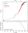 |
Fig. 2 Top panel: cumulative magnitude distribution N(< H) of the Datura family members. The black symbols are all 91 known members (including the largest asteroid (1270) Datura shown by the diamond, but disregarding (429988) 2013 PZ36, whose membership in the family is uncertain); the red symbols are 60 members detected by CSS during the phase 2 operations. The top abscissa indicates an approximate size computed from H with an assumption of pv = 0.24 value of the geometric albedo. Bottom panel: detection probability p(H) of Datura members as a function of H during the phase 2 operations of CSS based on analysis of geometric and photometric detection factors ran on a large synthetic population of Datura members. We find that p = 1 up to H ≃ 18 magnitude, which sets the limit where the Datura population is complete (dashed line on the upper panel). Beyond this limit p decreases to zero at about 21 magnitude. |
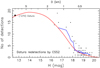 |
Fig. 3 Number of detections of the identified Datura family members during the phase 2 CSS operations: the largest body (1270) Datura shown by a diamond symbol and highlighted using a label, other 59 smaller members shown by black symbols. The red line is the theoretical prediction based on a large synthetic Datura population computed together with the detection probability p(H) from Fig. 2. The blue curve is a mean number of detections for the observed Datura members computed on a running window of 7 consecutive data-points. |
 |
Fig. 4 Osculating values of the secular angles – longitude of node Ω (abscissa) and longitude of perihelion ϖ (ordinate) – for members in the Adelaide family (epoch MJD 60 000.0). The black symbols show multiopposition orbits, gray symbols are for the singleopposition orbits; diamond symbol for (525) Adelaide, the largest member. The dashed line has the expected slope −0.5 (see, e.g., Figs. 1 and 9 for Datura and Rampo families), but the data are more scattered in the Adelaide case. This is likely due to Mars perturbation discussed in Vokrouhlický et al. (2021b). |
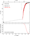 |
Fig. 5 Top panel: cumulative magnitude distribution N(< H) of the Adelaide family members. The black symbols are all 79 known members (including the largest asteroid (535) Adelaide shown by the diamond), the red symbols are 63 members detected by CSS during the phase 2 operations. The top abscissa indicates an approximate size computed from H with an assumption of pV = 0.24 value of the geometric albedo. Bottom panel: detection probability p(H) of Adelaide members as a function of H during the phase 2 operations of CSS based on analysis of geometric and photometric detection factors ran on a large synthetic population of Adelaide members. We find that p = 1 up to H ≃ 18.2 magnitude, which sets the limit where the Adelaide population is complete (dashed line on the upper panel). Beyond this limit p decreases to zero at about 20.4 magnitude. |
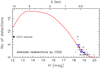 |
Fig. 6 Number of detections of the identified Adelaide family members during the phase 2 CSS operations: the largest body (525) Adelaide shown by a diamond symbol and highlighted using a label, other 62 smaller members shown by black symbols. The red line is the theoretical prediction based on a large synthetic Adelaide population computed together with the detection probability p(H) from Fig. 5. The blue curve is a mean number of detections for the observed Adelaide members computed on a running window of 9 consecutive data-points. |
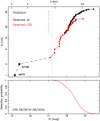 |
Fig. 7 Top panel: cumulative magnitude distribution N(< H) of the Hobson family members. The black symbols are all 60 known members (including the largest asteroids (18777) Hobson and (57738) 2001 UZ160 shown by the diamond), the red symbols are 33 members detected by CSS during the phase 2 operations. The top abscissa indicates an approximate size computed from H with an assumption of pV = 0.2 value of the geometric albedo. Bottom panel: detection probability p(H) of Hobson members as a function of H during the phase 2 operations of CSS based on analysis of geometric and photometric detection factors ran on a large synthetic population of Hobson members. We find that p = 1 up to H ≃ 17.2 magnitude, which sets the limit where the Hobson population is complete (dashed line on the upper panel). Beyond this limit p decreases to zero at about 19.5 magnitude. |
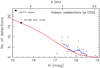 |
Fig. 8 Number of detections of the identified Hobson family members during the phase 2 CSS operations: the largest bodies (18777) Hobson and (57738) 2001 UZ160 shown by a diamond symbol and highlighted using a label, other 31 smaller members shown by black symbols. The red line is the theoretical prediction based on a large synthetic Hobson population computed together with the detection probability p(H) from Fig. 7. The blue curve is a mean number of detections for the observed Hobson members computed on a running window of 9 consecutive data-points. |
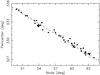 |
Fig. 9 Osculating values of the secular angles – longitude of node Ω (abscissa) and longitude of perihelion ϖ (ordinate) – for members in the Rampo family (epoch MJD 60 000.0). The black symbols show multiopposition orbits, gray symbols are for the singleopposition orbits; diamond symbol for (10321) Rampo, the largest member. Larger/smaller relative values of the secular angles, measured with respect to (10321) Rampo, correlated with positive/negative shift in proper semimajor axis. The node/perihelion trends are opposite, because the node drift in a retrograde sense, while the perihelion drifts in the prograde sense. The dashed line with a slope −0.5 indicates the correlation trend. |
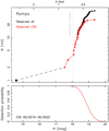 |
Fig. 10 Top panel: cumulative magnitude distribution N(< H) of the Rampo family members. The black symbols are all 42 known members (including the largest asteroid (10321) Rampo shown by the diamond), the red symbols are 26 members detected by CSS during the phase 2 operations. The top abscissa indicates an approximate size computed from H with an assumption of pV = 0.24 value of the geometric albedo. Bottom panel: detection probability p(H) of Rampo members as a function of H during the phase 2 operations of CSS based on analysis of geometric and photometric detection factors ran on a large synthetic population of Rampo members. We find that p = 1 up to H ≃ 18 magnitude, which sets the limit where the Rampo population is complete (dashed line on the upper panel). Beyond this limit p decreases to zero at about 20 magnitude. |
3.2 Extremely young asteroid families with small numbers of known members
Wasserburg. A very tight asteroid pair of two Hungaria objects (4765) Wasserburg and 2001 XO105 was reported by Vokrouhlický & Nesvorný (2008). Pravec et al. (2010), analyzing the formation process of asteroid pairs, included this couple in their sample and reported an approximate age larger than 90 kyr. Pravec et al. (2019), compiling the most detailed study of the asteroid pair population, noted a small asteroid 2016 GL253 accompanying the pair on a very close orbit and suggested the trio of asteroids may be the large-end tip of a very young family in the Hungaria population. Novaković et al. (2022) confirmed the trend, detecting six members in what they called the Wasserburg family. Here we find two more members in the family, completing the count at Nobs = 8. Interestingly, all of them were also detected during phase 2 of the CSS operations, thence NCSS = 8.
The cumulative magnitude distribution of the presently known members of the Wasserburg family is shown in Fig. 12. The bottom panel on the same figure provides the detection probability p(H) during CSS phase 2 operations. The completion limit is near H ≃ 18.5 magnitude, impressively large in spite of the high inclination of the Wasserburg family orbits (being part of the Hungaria zone). Some of these orbits may be missed by the fields-of-view of CSS. The situation improved after July 2016, however, with the wide field camera reaching well beyond the ±30° zone around the ecliptic. So the geometric losses are small, and the heliocentric proximity of the Hungaria region helped to detect even small asteroids. Indeed, the six smallest members in the Wasserburg family have an absolute magnitude near or even above the H = 19 limit.
As mentioned in the preamble of this section, the small number of identified members in this family does not permit a full-scale debiasing effort. Accordingly, we only conducted the simplest estimate to characterize the complete Wasserburg population using the following steps:
We considered the observed (biased) population of the family members and sorted their absolute magnitude values {Hi}, with i = 1,…, Nobs, from the smallest to the largest value;
By definition, the observed population increases by one when shifting along the list according to the ordered H-values; we assume the largest member in the family is bright enough such that p(H1) = 1;
The simplest estimate of the complete population is then obtained by again moving along the vector {Hi} of ordered absolute magnitudes, but now incrementing the population by 1/p(Hi) instead of one.
The result is shown by the blue curve at the top panel of Fig. 12. Since even the smallest Wasserburg fragment has p(H8) ≃ 0.71 (in other words, detection of even the smallest known fragments is expected), the complete population does not deviate too much from the observed population. Up to that point the cumulative magnitude distribution is very steep, locally approximated by a power law with an exponent of γ ≃ 1.4. This value is only slightly shallower than that observed in the case of the Adelaide family. From that similarity, we may tentatively conclude that Wasserburg family has resulted from a huge cratering event in (4765) Wasserburg itself, though again there are many additional possibilities (e.g., Durda et al. 2007).
However, an outstanding puzzle here is to explain why the current surveys have yet to detect any smaller fragments. This reason is because of the inferred steepness of the magnitude distribution, and the non-negligible detection probability p(H8) mentioned above. In other words, a fair number of the subsequent members in the Wasserburg family should have a detection probability ≃0.5, yet none have been detected. Does this mean that the magnitude distribution beyond the detected population suddenly becomes shallow. The answer to this question is left for future analysis.
Martes. Vokrouhlický & Nesvorný (2008) mentioned (5026) Martes and 2005 WW113 among their list of tight asteroid pairs. As also noted by these authors, some of these pairs were expected to be the two largest members in a collisionally born asteroid family (e.g., Wasserburg family). Recently, Novaković et al. (2022) reported a third member in the tight orbital region about Martes, namely 2010 TB155, while our census in this paper increases the number by three more small objects, with Nobs = 6 (Table A.6), with the last three asteroids associated with the Martes cluster discovered in Autumn 20225. Only the largest three members in the Martes family were detected by CSS, such that NCSS = 3. The Martes cluster is a part of a much larger Erigone family, whose age has been estimated to ≃280 Myr (e.g., Vokrouhlický et al. 2006; Spoto et al. 2015) or 130 ± 30 Myr by Bottke et al. (2015b). This association is justified by the objects having the same spectral taxonomic type Ch as the Erigone family and (5026) Martes (Polishook et al. 2014). The extremely clustered orbital elements of the Martes members suggest an unusually young age for the family. Indeed, Pravec et al. (2019) found 18 ± 1 kyr, a slight improvement on the result of Pravec et al. (2010). We find that the orbits of the smallest three members may also converge to this time window, further justifying the Martes age, but a detailed analysis would need to consider the thermal accelerations in the simulation. We leave this effort to a separate study, but conclude here that the Martes family has the youngest currently known age.
Figure 13 shows the absolute magnitude distribution of the Martes family members. Admittedly this distribution is an incomplete portion of the family population, and for that reason we do not attempt a serious debiasing effort. We only note the behavior of the detection probability p(H) determined for the phase 2 operations of CSS (bottom panel of Fig. 13). Martes-family orbits have the largest eccentricity among our sample, and this produces the largest stretch of H values in which p(H) decreases from 1 to 0. At magnitude H ≃ 20 we have p ≃ 0.1.
Taken at a face value, we would infer a large population of small members in the Martes family, such that every one of the three may represent in fact ≃ 1/p ≃ 10 asteroids. This logic might be flawed, however, because the three small members were not detected by phase 2 CSS. Strictly speaking, we should not use them to infer anything about Martes family magnitude distribution. Nevertheless, we believe our inferences may be close to reality. This is because all three smallest asteroids in the Martes family were detected by G96/CSS in September 2022. This time period is technically out of the phase 2 interval, but only by a small amount. It also shows the capability of G96 to detect them. The size of the Martes population at H ≃ 20 is left for future work.
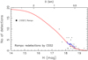 |
Fig. 11 Number of detections of the identified Rampo family members during the phase 2 CSS operations: the largest body (10321) Rampo shown by a diamond symbol and highlighted using a label, other 25 smaller members shown by black symbols. The red line is the theoretical prediction based on a large synthetic Rampo population computed together with the detection probability p(H) from Fig. 10. The blue curve is a mean number of detections for the observed Rampo members computed on a running window of 9 consecutive data-points. |
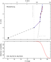 |
Fig. 12 Top panel: cumulative magnitude distribution N(< H) of the Wasserburg family members. The black symbols are all 8 known members (including the largest asteroid (4765) Wasserburg shown by the diamond), the blue symbols provide the simplest variant of the debiased population. This was obtained by incrementing the population by 1/p(Hi+1), when stepping from absolute magnitude Hi to Hi+1 (i = 1,…,Nobs); the observed (biased) population increments by one by definition. The gray line is an approximate local power-law representation N(< H) ∝ 10γH near H ≃ 19 with γ ≃ 1.4. The top abscissa indicates an approximate size computed from H with an assumption of pV = 0.3 value of the geometric albedo. Bottom panel: Detection probability p(H) of Wasserburg members as a function of H during the phase 2 operations of CSS based on analysis of geometric and photometric detection factors run on a large synthetic population of Wasserburg members. We find that p = 1 up to H ≃ 18.3 magnitude, which sets the limit where the Wasserburg population is complete (dashed line on the upper panel). Beyond this limit p decreases to zero at about 20.5 magnitude. |
3.3 Starving young asteroid families with only three known members and asteroid pairs
Lucascavin. This very tight cluster of three asteroids was discovered by Nesvorný & Vokrouhlický (2006), who also estimated its age to 300–800 kyr (the large uncertainty is due to small size of the two small members – see Table A.7 – and unconstrained magnitude of the thermal accelerations in their orbit). A decade later, Pravec et al. (2018) found the three original members were still the only ones in this cluster. They also calculated its age to be between 500 and 1000 kyr using a different method. Assuming the population is complete, these authors also argued that the estimated sizes of the Lucascavin members, and the ≃5.79 h rotation period, might be enough for rotation fission of the parent object to explain their origin (e.g., Pravec et al. 2010, 2019). The difference with respect to the population of pairs is that the assumption that the secondary, escaping from the primary after the fission event, would split into two components (namely the two small members (180255) 2003 VM9 and (209570) 2004 XL40). This possibility was theoretically predicted by Jacobson & Scheeres (2011). If, however, numerous smaller fragments are found in the Lucascavin family, this scenario would become less plausible. Therefore, unlike our study of other clusters in this paper, the goal of our analysis here is to “disprove” the existence of further fragments in the family. Obviously, we cannot meet this goal in an absolute manner, but we can set a lower limit on the absolute magnitude of a putative companion (or, in other words, an upper limit on its size).
Moving towards that goal, we note that all three known members in the Lucascavin family were detected during both phases 1 and 2 of the CSS operations (in our notation, we thus have Nobs = 3 and NCSS = 3)6. In order to use as much information as possible, we have combined data from both phases of the CSS operations. Given their different performance, we consider both phases as independent (and uncorrelated) sources of information. Denoting then the detection probability during the phase 1 by p1, and similarly the detection probability during the phase 2 by p2, the combined total detection probability p during both phases is
 (1)
(1)
Note that we first characterized the non-detection during both phases (the second term), and then take the complement to unity, which expresses detection in at least one of the CSS phases. Results are shown in Fig. 14.
We first briefly comment on the behavior of p1 and p2 (the blue and red curves). The interesting, and at the first sight puzzling, feature of p1 is that it does not reach a value of 1 even for rather bright objects (its maximum value is only about 0.9). This is not a mistake, but the result of the Lucascavin cluster’s semimajor axis. The synodic period of its motion with respect to an Earth observer is in an approximate 7:5 resonance over a year. As a result, for a survey spanning only a short period of time (such as little more than 3 yr of our CSS phase 1 operations), it may happen that Lucascavin objects with certain values of mean longitude in orbit λ never occur in the field-of-view (reasonable solar elongations on the night sky). Since this is a purely geometrical effect, it affects the detection probability of even very bright objects (see, e.g., Tricarico 2017, Fig. 2 for illustration of this effect for near-Earth object characterization). As the duration of the survey extends, this effect minimizes and even disappears. As a result, p2 in the 6 yr interval of CSS phase 2 (red curve) does not suffer from this problem. The overall detection probability p1 is smaller than p2, but both reach p1 ≃ p2 ≃ 0 at similar H ≃ 20.5. This outcome is because the apparent magnitude detection limit is similar for both phases.
Following the trend of the black curve of Fig. 14, p(H), we note that p(H) ≃ 1 up to H ≃ 18.3. Therefore the Lucascavin population is complete to this magnitude limit. This calculation is a conservative estimate because observations of other surveys may push this limit to higher values. The limit is about one magnitude larger than that of the two small members in the Lucascavin family (≃17.25). Our result may be therefore interpreted in two ways: either (i) it sets a constraint on Lucascavin family magnitude distribution, or (ii) it starts tracing the population void beyond the known set. The former case would imply at least a magnitude gap between the third and the fourth largest members in the family (this is not impossible, see, e.g., Fig. 2). The latter case may support the idea that the Lucascavin family formed by rotation fission, with the secondary disrupting into two pieces.
Rheinland and Kurpfalz. The pair of asteroids composed of a primary (6070) Rheinland and a secondary (54827) Kurpfalz is the best studied archetype in its class. This is because the two asteroids are rather large, namely the D1 ≃ 4.4 ± 0.6 km size primary and the D2 ≃ 2.2 ± 0.3 km size secondary (absolute magnitudes H1 = 14.17 ± 0.07 and H2 = 15.69 ± 0.04), and reside in the inner part of the asteroid belt. Their discoveries in 1991 and 2001, and prediscovery data extending to 1950 and 1991, imply a wealth of astrometric observations allowing accurate orbit determination. This has been noticed already by Vokrouhlický & Nesvorný (2008), who used this pair to demonstrate they could reach full convergence in Cartesian space of the two orbits in the past. From this result, they determined the pair had an age of ≃ 17 kyr. Later, Vokrouhlický et al. (2011, 2017b) conducted photometric observations of both asteroids with the goal to determine their rotation state, including pole orientation, and shape model. Intriguingly, the spin orientation at the likely moment of their formation has not been found to be parallel for the two components, but instead is slightly tilted by about 38°. The well confined spin state for both components in this pair allowed them to pin down the formation epoch to 16.34 + 0.04 kyr (see Vokrouhlický et al. 2017b). An interesting clue about the formation process, fission of a critically rotating parent body (e.g., Pravec et al. 2010, 2019), is also provided by spectroscopic observations of Rheinland and Kurpfalz: while the first has been found a typical S-class object, the taxonomy of the latter is either Sq- or even Q-class (see Polishook et al. 2014).
Similarly to the case of the Lucascavin family, we aim to determine the magnitude limit for nonexistence of a putative companion fragment following Rheinland and Kurpfalz on their heliocentric orbit. Since both Rheinland and Kurpfalz were detected during CSS phases 1 and 2, we may again combine detection probabilities p1 and p2 to obtain the total probability p according to the formula (1). Results are shown in Fig. 15.
In this case, p1 is comfortably close to unity even for the fainter component (54827) Kurpfalz7. However, p1 starts dropping to zero right after H2 of the secondary, such that limited useful information would have been reached if we only had the phase 1 data. Luckily, the power of the CSS phase 2 observations make extending the final detection probability p for the orbits in this pair to unity, even near H ≃ 18. We may thus conclude that the available observations rule out a companion fragment of this pair to this limit, which is ∆H ≃ 2.3 larger than H2 of the secondary. Assuming the same albedo, the hypothetical companion – if it exists – must have a size smaller than ≃ 10−0.2∆H D2 ≃ 0.8 km.
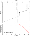 |
Fig. 13 Top panel: cumulative magnitude distribution N(< H) of the Martes family members. The black symbols are all 6 known members (including the largest asteroid (5026) Martes shown by the diamond). The top abscissa indicates an approximate size computed from H with an assumption of pV = 0.06 value of the geometric albedo (conforming the Ch-class taxonomy). Bottom panel: detection probability p(H) of Martes members as a function of H during the phase 2 operations of CSS based on analysis of geometric and photometric detection factors run on a large synthetic population of Martes members. We find that p = 1 up to H ≃ 17.5 magnitude, which sets the limit where the Martes population is complete (dashed line on the upper panel). Beyond this limit p decreases to zero at about 20.5 magnitude. At magnitude ≃20 p ≃ 0.1. This implies that the three very small members recently detected must represent a tiny sample of a much larger population having about the same size. |
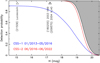 |
Fig. 14 Detection probability of an additional small fragment in the Lucascavin family: (i) the blue curve is p1 during the phase 1 of CSS operations, and (ii) the red curve is p2 during the phase 2 of CSS operations. The black curve is the combined probability p during both phases (Eq. (1)). The gray area allows the existence of an additional small body in the system, whose maximum probability of occurrence is complementary value to the probability p on the left ordinate. |
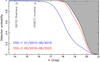 |
Fig. 15 Detection probability of a companion to Rheinland and Kurpfalz on their heliocentric orbit: (i) the blue curve is p1 during the phase 1 of CSS operations, and (ii) the red curve is p2 during the phase 2 of CSS operations. The black curve is the combined probability p during both phases (Eq. (1)). The gray area allows the existence of an additional small body in the system, whose maximum probability of occurrence is complementary value to the probability p on the left ordinate. |
4 Results
We now proceed towards a more advanced debiasing method than previously used in the case of the Wasserburg family. The four families introduced in Sect. 3.1 with large-enough known population of members – Datura, Adelaide, Rampo and Hobson – will serve us as our testbed cases.
The method, in essence similar to what has been used by Vokrouhlický et al. (2017a), goes as follows:
First, we consider the CSS phase 2 detected sample
 (i = 1,…, NCSS) of the family asteroids and we select a certain member
  for which
  (we call it a “branching point”). We assume that the population is complete up to the absolute magnitude of that member and becomes incomplete for magnitudes larger than
  . The cumulative magnitude distribution is therefore represented by the observed population until
  , where it has N1 members, and then continued with a synthetic (model) population as described below. We also denote the number of family members with magnitudes
  detected during the CSS phase 2 by
  .
.Second, we generated the total synthetic population of family members
 having absolute magnitudes in between
  and a certain value H2 sufficiently larger than
  with a statistical distribution of the tested magnitude distribution function (we use the sequence of ℳ models described below and always order the magnitude sequence from the smallest to the largest).
Third, we used the detection probability p(H) of the CSS observations to transform the total synthetic population to the biased synthetic population
 , such that each of
  is consulted as to its detectability. In practice, for each
  we evaluated
  and compared it to a uniformly random number r between 0 and 1, providing a rationale for detectability or non-detectability: (i) if
  , the asteroid is deemed detected and we record
  in the
  sequence, and (ii) if
  , the asteroid is deemed not detected and we proceed to the next
  value.
-
Fourth, we evaluated a chi-square type target function
 (2)
(2)comparing the modeled and biased magnitude distribution to the detected set
 by CSS beyond the branching magnitude
  .
.
For sake of simplicity, we (i) use σi; = 0.1 magnitude for all bodies, and (ii) adopt Gaussian statistics to judge the goodness-of-the-fit and set confidence limits on the adjusted parameters of the model needed to construct the complete (not-biased) synthetic population  . As for the synthetic population, we use the following sequence of power-law models:
Model ℳ1 – a straight single-slope power law N(< H) ∝ l0γH with one adjustable parameter γ (the absolute normalization for all ℳ-models is set by number N1 = N(< H1) of family asteroids at H1, because we make sure that the population is complete to that limit);
Model ℳ2 – a broken power-law model with one adjustable break-point at Hbreak (H1 ≤ Hbreak ≤ H2) and two adjustable slope exponents γ1 and γ2 for H values in the intervals (H1, Hbreak) and (Hbreak, H2) respectively;
Model ℳ3 – a broken power-law model with two adjustable break-points at Hbreak,1 and Hbreak,2 (H1 ≤ Hbreak,1 < Hbrea,2 ≤ H2) and three adjustable slope exponents γ1, γ2 and γ3 for H values in the intervals (H1, Hbreak,1), (Hbreak,1, Hbreak,2) and (Hbreak,2, H2) respectively;
and similarly for ℳi model with 2i − 1 parameters (i − 1 break-points and i slopes for the intermediate intervals of H). In practice, we limit ourselves to ℳ3 at maximum in this paper.
Denote p the set of model parameters (e.g., p = (Hbreak, γ1 ,γ2) for the ℳ2 model). Since χ2 = χ2(p) in (2), the usual goal is to minimize its value by selecting the best-fit p⋆ parameter choice. We use a simple Monte Carlo sampling of p space to find these values and to map χ2 behavior within some zone about the minimum value  . The confidence limits on p are found by choosing a certain domain with a threshold
  . For instance, the 99% confidence limit in one, three and five parametric degrees of freedom in ℳ1, ℳ2 and ℳ3 models corresponds to Δχ2 = 6.63, 11.3 and l5.1 respectively (e.g., Press et al. 2007). Similarly the measure of the goodness-of-fit is judged from the
  value using the incomplete gamma function as discussed in Press et al. (2007).
Datura. Considering the data in Fig. 1 we chose j = 9 in the case of the Datura family, namely taking the absolute magnitude  of the ninth family member as the branching point (i.e.,
  in this case). We will test the ℳ1 and ℳ2 models8.
In the former case, we find  (99% confidence level) and the best-fit solution having
  . In the latter case, we find
  , and
, and  (99% confidence level) and the best-fit solution having a significantly improved
  (the improvement for the ℳ3 model is already statistically insignificant).
The best-fit solutions of both models are shown in Fig. 16. While formally the minimum  values are both statistically justifiable using the Q-function measure (Press et al. 2007), the ℳ1 performs quite worse beyond H ≃ 19.5. This is because continuing the steep power-law distribution required by the magnitude distribution of the Datura members between H = 18 and 19 would keep pushing the detactable population high (given the only slow decay of the detection probability p(H) from Fig. 1). This problem is remedied by setting a break-point at which the distribution becomes shallower; this behavior is readily provided by the ℳ2 model. The upper abscissa on both panels of Fig. 16 is an estimate of Datura member size using the geometric albedo value pV = 0.24. The break-point magnitude Hbreak solution within the ℳ2 model maps onto a 0.3–0.5 km range of sizes.
Figure 17 provides more detailed information on the ℳ2 model parameter solution. In spite of weak correlations, the solution seems to be well-behaved. Interestingly, the slope exponents satisfy γ1 > 0.6 and γ2 < 0.6. The magnitude slope γ translates to an exponent α = −5γ of a cumulative size distribution (assuming constant albedo on a given interval of H-values). Therefore the threshold value 0.6 maps onto a critical size exponent −3: for shallower distributions the mass is dominated by the largest members, while for steeper distributions the mass is dominated by the smallest fragments.
In our ℳ2 solution for Datura members, the mass is dominated by the sizes at the breakpoint, while in the ℳ1 solution the fragment mass cannot be well constrained because it is dominated by the smallest members. Here we use the ℳ2 solution and estimate the total mass mfrag contained in Datura family members with absolute magnitudes between 16 and 20 from our complete model (i.e., excluding (1270) Datura itself). We also normalize mfrag by the mass mLF of (1270) Datura. The statistical distribution of this ratio, as mapped from the 99% confidence level parametric region shown in Fig. 17, is shown in Fig. 18. We find  . Unless the cumulative number of Datura members becomes significantly steeper somewhere beyond the magnitude limit 20, which is certainly possible (e.g., Durda et al. 2007), we estimate that their collective mass only represents ≃3.3% of the (1270) Datura mass. From this analysis, we suggest the family may have been formed from a large cratering event.
Adelaide. The extreme nature of the magnitude distribution in the Adelaide family (Fig. 4) makes us choose j = 2, therefore we associate the point to the first member next to (525) Adelaide with  . With that choice we have
  . In this case, we test ℳ1, ℳ2 and ℳ3 models.
We find that the single power-law model ℳ1 is incompatible with the family data. The formally best-fit slope γ ≃ 1.86 tries to compromise between the extremely steep part of the magnitude distribution between 18.18 and ≃ 18.75 and much shallower distribution beyond. However, none of the features is matched well and the formal  has to be statistically rejected. The basic inconsistency of such a model stems from the behavior of the detection probability p(H) shown in the bottom panel of Fig. 4. In simple words, p(H) is quite smooth and gradual even beyond ≃19 magnitude and does not resemble the sharp lack of detected fragments at ≃18.7 magnitude. In the Adelaide family case, we need some slope change even in the complete population, and this is provided by models ℳ2 and ℳ3.
In the former case, we find  (99% confidence level). The bestfit solution has
  . The model reflects a slope change from steep to shallow near 18.75. The minimum of χ2 reached in the ℳ2 model is fully acceptable, yet the left panel on Fig. 19 indicates the solution may still be improved (obviously at the expense of more parameters). This is provided by the ℳ3 model (the right panel on Fig. 19), which has
  (99% confidence level) and has
  .
.
Figure 20 shows 2D projections of the ℳ2 model parameters, resembling those for Datura family in Fig. 17, except for γ1 value significantly steeper. The ℳ3 model parameters are more correlated within each other, as many combinations for positions of the two breakpoints Hbreak,1 and Hbreak,2 and the intermediate slopes γ1 and γ2, are possible. Obviously, the solution of the faintest-slope γ3 is consistently shallow, even shallower than γ2 in model ℳ2 (see Fig. 20).
There is a robust, common result following from the ℳ2 and ℳ3 models: (i) the initial slope parameter in the 18.2–18.6 absolute magnitude range must be very steep (i.e., 2–3, and (ii) the final slope beyond absolute magnitude 19 must be rather shallow (i.e., 0.1–0.7). Given the shallow magnitude distribution at the limit of very small Adelaide members (for most part < 0.6), the bias-corrected fragment population mass is dominated by H ≃ 19 Adelaide members. We can thus repeat the computation performed for the Datura family, and compute the ratio mfrag/mLF of the Adelaide members with H > 18 (mfrag) and the mass of the largest asteroid (525) Adelaide itself (mLF). Obviously, we carry out this computation for the bias-corrected populations of the ℳ2 and ℳ3 models, rather than the observed population of the Adelaide family members.
The results, shown in Fig. 21, provide tight constraints on the complete population of the Adelaide members in the 18–20 magnitude range:  for the ℳ2 model, and
  for the ℳ3 model. If these estimates hold also for the population at the family origin (see Sect. 5 for an alternative option), the Adelaide family is an exemplary case of a large cratering event. We estimated the size of the expected crater on (525) Adelaide in Sect. 5.
Rampo. In this case, we use j = 4, corresponding to a  magnitude branching point (Fig. 10). Using that choice we have
  , slightly less data than for the Datura and Adelaide families. We tested the ℳ1 and ℳ2 models in this situation.
The best-fit with a single power-law ℳ1 model only reaches  (with the median slope parameter γ ≃ 1.44). Given
  data points, this solution is statistically unacceptable (the quality factor Q ≃ 0.067; see Press et al. 2007). Figure 22 illustrates the problem in a graphical way, namely the predicted population of fragments beyond magnitude 19 (blue dashed line on the left panel) becomes steep and incompatible with the single Rampo fragment detected by CSS. Things improve if the magnitude of the power-law model ℳ1 is shifted to
  (still within the assumed 0.1 magnitude uncertainty). This helps to straighten the sequence of observed members immediately after
  , where the detection probability is still close to 1. With that change, the single power-law model ℳ1 provides best match with
  (and, obviously, smaller slope γ ≃ 1.17). While not impressive, the solution is formally acceptable, but it suffers from the same problem in matching the faint end of the observed Rampo population using CSS.
The broken power-law model ℳ2 performs much better in this circumstance. It reaches  , and the parameter solution
  (99% confidence level; see Fig. 23). The overall median slope ≃1.17−1.44 is thus traded for a steeper leg initially, followed with a shallower part beyond Hbreak. The small
  conforms to the visually perfect match shown on the right panel of Fig. 22.
Figure 24 shows the model predicted mass in the Rampo members between magnitudes 18 and ≃ 19.5, namely  . However, since the γ2 slope beyond Hbreak tends to be steep (with value larger than 0.6 not excluded), the real fragment mass with respect to (10321) Rampo may be even larger. In any case, out of the three families analyzed so far, the Rampo family represents the most energetic collisional event.
Hobson. The record of observed Hobson members, both the total count and the subset detected by CSS, is comparable to the Rampo family. However, because of Hobson’s larger heliocentric distance, and its larger eccentricity, the predicted detection probability by CSS is shifted by nearly a magnitude towards small H values (see Figs. 7 and 10). This allows us to conduct the bias-correction on a shifted segment of Hobson member magnitudes/sizes if compared to Rampo, which explains the differences in results.
In this case, we use j = 3, corresponding to the  magnitude branching point (Fig. 7). Using that choice, we have N′CSS = 31. We tested the ℳl and ℳ2 models in this situation.
Given the aforementioned difference in detection probabilities for the Rampo and Hobson families, the ℳl model is currently sufficient to match the Hobson population between ≃ 17 and ≃ 19 magnitudes (Fig. 25). The best-fit simulation reaches  , while the simulations using the ℳ2 model were able to improve this value to
  . This is not enough of a statistically significant difference to justify the necessity of a broken power-law model for the Hobson population of members; the simple power-law model performs just as well. The slope parameter is
  (99% confidence level). Because this value is larger than 0.6, we cannot estimate the mass contained in the fragment population, (as the smallest asteroids still dominate the mass). We can only set a lower limit from the population available to us, and this gives mfrag/mLF ≥ 0.6. In this case, mLF contains the mass of the two largest asteroids, (18777) Hobson and (57738) 2001 UZ160. Clearly, the Hobson family results from the catastrophic disruption of a parent body.
 |
Fig. 16 Best-fit solution of the complete Datura population to the magnitude limit H2 = 20 and its comparison to the observed population. Left panel: the single power law ℳl model with the free parameter representing the slope γ. The best fit value is γ = 0.70, and the corresponding |


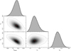 |
Fig. 17 Admissible parameter values of the ℳ2 broken power-law model approximating Datura family absolute magnitude distribution in the range H e (H1, H2) = (18.09, 20). There are three solved-for parameters in the model: (i) the break-point magnitude Hbreak, (ii) the power-law exponent γ1 for H ≤ Hbreak, and (iii) the power-law exponent γ2 for H ≥ Hbreak. Each of the panels shows a projection of the solution onto different 2D subspaces of the 3D space of parameters (Hbreak,γ1,γ2). The dashed line delimits 99% confidence limit zone of the solution, and the gray-scale is proportional to the probability density distribution of the solutions. The best-fit parameter combination is shown by red star symbol. The gray histograms are simply 1D probability density distributions for each of the parameters on the abscissa. The dotted line at γ1 or γ2 values of 0.6 is shown for reference. |
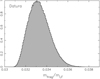 |
Fig. 18 Probability density distribution of the ratio mftag/mLF (normalized to unit at maximum), where mfrag is the mass/volume of all members up to absolute magnitude 20 without (1270) Datura, and mLF is the mass/volume of the largest member (1270) Datura. Solution using the broken power-law model ℳ2. |
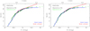 |
Fig. 19 Best-fit solution of the complete Adelaide population to the magnitude limit H = 20 and its comparison to the observed population. Left panel: the broken power-law model ℳ2 with three adjustable parameters (Hbreak, γ1, γ2). The best-fit values (red star in Fig. 20) are: Hbreak = 18.78, γ1 = 2.08, and γ2 = 0.47, and the corresponding |


 |
Fig. 20 Admissible parameter values of a ℳ2 broken power-law model approximating Adelaide family absolute magnitude distribution in the range H ∈ (H1, H2) = (18.2, 20). There are three solved-for parameters in the model: (i) the break-point magnitude Hbreak, (ii) the power-law exponent γ1 for H ≤ Hbreak, and (iii) the power-law exponent γ2 for H ≥ Hbreak. Each of the panels shows a projection of the solution onto different 2D subspaces of the 3D space of parameters (Hbreak, γ1, γ2). The dashed line delimits 99% confidence limit zone of the solution, and the gray-scale is proportional to the probability density distribution of the solutions. The best-fit parameter combination is shown by red star symbol. The gray histograms are simply 1D probability density distributions for each of the parameters on the abscissa; the dashed histograms along the distributions of the γ1 and γ2 exponents correspond to the first and the last exponent in the ℳ3 broken power-low models with two break-points (Hbreak,1, Hbreak,2; i.e., the first in the interval (18.2, Hbrκak,1), and the second in the interval (Hbreak,2, 20)). The dotted line at γ1 or γ2 values of 0.6 is shown for reference. |
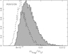 |
Fig. 21 Probability density distribution of the ratio mfrag/mLF (normalized to unit at maximum), where mfrag is the mass/volume of all members up to absolute magnitude 20 without (525) Adelaide, and mLF is the mass/volume of the largest asteroid (525) Adelaide. The solid/gray histogram for the ℳ2 model, the dashed histogram for the ℳ3 model (all models whose parameters p are within the 99% confidence level of the family population were used). |
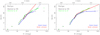 |
Fig. 22 Best-fit solution of the complete Rampo population to the magnitude limit H2 = 20 and its comparison to the observed population. Left panel: the single power law ℳl model with the free parameter representing the slope γ. The best fit value is γ ≃ 1.17, and the corresponding |


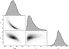 |
Fig. 23 Admissible parameter values of the ℳ2 broken power-law model approximating Rampo family absolute magnitude distribution in the range H ∊ (H1, H2) = (18.1, 20). There are three solved-for parameters in the model: (i) the break-point magnitude Hbreak, (ii) the power-law exponent γ1 for H ≤ Hbreak, and (iii) the power-law exponent γ2 for H ≥ Hbreak. Each of the panels shows a projection of the solution onto different 2D subspaces of the 3D space of parameters (Hbreak, γ1, γ2) The dashed line delimits 99% confidence limit zone of the solution, and the gray-scale is proportional to the probability density distribution of the solutions. The best-fit parameter combination is shown by red star symbol. The gray histograms are simply 1D probability density distributions for each of the parameters on the abscissa. The dotted line at γ1, or γ2 values of 0.6 is shown for reference. |
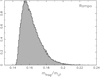 |
Fig. 24 Probability density distribution of the ratio mfrag/mLF (normalized to unit at maximum), where mfrag is the mass/volume of all members up to absolute magnitude 20 without (10321) Rampo, and mLF is the mass/volume of the largest asteroid (10321) Rampo. Solution using the broken power-law model ℳ2. |
5 Discussion and conclusions
Our work provides evidence for a break in the magnitude distribution in several of the very young families analyzed here. Before considering implications, however, we first must attempt to further justify the result and understand its meaning. We can think of at least two conventional reasons for what we see.
Missing halo of small members? The first possibility is that we were unable to identify small family members beyond Hbreak. Their deficit, quantitatively as shown by the shallow slope at faint magnitudes, may not be real, but instead represents a failure in our the clustering association. Perhaps, many of these small fragments were ejected with larger velocities and drifted farther from the core of the family. This scenario is a plausible situation for larger and older families in the main belt, which are identified in 3D proper element space by their large spatial densities of asteroids compared to the background population (see discussion in Nesvorný et al. 2015). For the very young families, however, clusters in the 5D space of osculating orbital elements, with additional tracers such as the correlated values of the secular angles Ω and ϖ (Sect. 3), help to minimize the problem of missing members (if identified in our catalogs). The nominal family-identification method, described in the Appendix, uses a very conservative search zone (followed by a control on the past convergence of the orbits). In order to demonstrate the margin we allow, we present a more in-depth test in the case of the Adelaide family here.
We use four nested boxes around the asteroid (525) Adelaide in osculating orbital elements (data from MPC catalog as of May 15, 2023), with the following parameters:
Box 1 defined by the following differences in semimajor axis a, eccentricity e, inclination I, longitude of node Ω, and argument of perihelion ω: (δa, δe, δI, δΩ,δω) = (±0.01, ±0.01, ±0.1°, 10°, 10°);
Box 2 defined by the following differences in semimajor axis a, eccentricity e, inclination I, longitude of node Ω, and argument of perihelion ω: (δa, δe, δI, δΩ,δω) = (±0.02, ±0.02, ±0.15°, 20°, 20°);
Box 3 defined by the following differences in semimajor axis a, eccentricity e, inclination I, longitude of node Ω, and argument of perihelion ω: (δa, δe, δI, δΩ,δω) = (±0.03, ±0.03, ±0.2°, 30°, 30°);
Box 4 defined by the following differences in semimajor axis a, eccentricity e, inclination I, longitude of node Ω, and argument of perihelion ω: (δa, δe, δI, δΩ,δω) = (±0.035, ±0.035, ±0.25°, 35°, 35°).
Our nominal procedure described in the Appendix uses Box 3, where we identified all 79 Adelaide family members listed in Table A.2. Here are the data of asteroid populations found in the subsequent boxes: (i) Box 1 contains 74 asteroids, all Adelaide family members and no background objects, (ii) Box 2 contains 84 asteroids, all 79 Adelaide family members and 5 background objects, (iii) Box 3 contains 105 asteroids, all 79 Adelaide family members and 26 background objects, and (iv) Box 4 contains 135 asteroids, all 79 Adelaide family members and 56 background objects. The identified members of the Adelaide family reside in the interior two boxes (for most part already in Box 1). The background population of asteroids slowly ramps from the Box 2 stage9. These statistics make us believe that we are not missing any distant (and small) Adelaide members. A similar situation applies to other families as well.
Collisional comminution of family members beyond Hbreak? The bias-corrected population of the family members, as follows from our analysis, tells us about the current population several hundreds of thousands of years after the origin of the clusters. This population may have experienced some degree of collisional evolution over that interval, enough to disrupt some family members. As a result, we must verify whether the transition to a shallower magnitude distribution beyond Hbreak in the case of the Datura, Adelaide and Rampo families is not simply produced by collisional comminution.
We note that the size distribution of the main belt becomes shallow below 1 km in diameter, and its equivalent steepness at ≃ 500 m may be as small as γ ≃ 0.3 (see Fig. 1 in Bottke et al. 2020). Any submerged population introduced into this vast population of projectiles, such as a volume-limited new family, tends to equilibrate with the background (assuming disruption laws are the same for the background and family objects). The crucial issue with young asteroid families is the timescale of this process: has enough time passed since the origin of the family to reach equilibrium for members that are hundreds of meters?
In order to explore this issue we performed the following numerical experiment. We used the well-tested Monte Carlo code Boulder (e.g., Morbidelli et al. 2009; Vernazza et al. 2018) to track the collisional evolution of multiple small-body populations. Here we simulated both the internal impact/cratering/disruption processes within each of the populations and also the mutual collisional interaction of the populations (i.e., objects in one population may serve as impactors for the other and vice versa). The code version we adopted models the size-frequency distribution for each of the populations but does not include the orbital dynamics of the population members.
We used two populations: (i) the background population of main belt asteroids taken from Bottke et al. (2015a), and (ii) the young family population. We were only interested in a briefinterval of time lasting ≤ 1 Myr (i.e., equal to the estimated age for the corresponding family).The origin of the simulation was the formation epoch of the family. The main belt population is effectively in equilibrium for the relevant sizes of about ten meters and larger, but the family population is expected to evolve with time; proving or disproving changes of the family size distribution at hundred meter and larger sizes was the goal of our simple test.
The initial size distribution of the family was equal to the best-fitting, bias-corrected solution from Sect. 4 with the following modification: we disregarded the breakpoint at Hbreak in the ℳ2 (and higher) class of solutions and continued the distribution with the power-exponent γ1 from the first magnitude interval (H1 , Hbreak). We considered 0.24 geometric albedo to convert absolute magnitude in Sect. 4 to sizes. Finally, we needed to specify parameters of the collisional interaction – intrinsic collisional probability pi and mean relative velocity  at impact – within each of the populations and across them. This was done as follows.
The intrinsic values of pi and  of the main belt population have been evaluated in many previous studies, and there is some small variation among them (related mostly to the smallest-size bodies used for their determination). We used pi = 2.9 × 10⁻¹⁸ km−2 yr−1 and
  = 5.3 km s−1 (see Sect. 2.1 in Bottke et al. 2015a). For simplicity, the same values were taken for main belt projectiles impacting the young asteroid family population. The latter was deemed to be negligible in the relevant sizes of ten meters and larger (see Fig. 27), which allowed us to neglect family members as a meaningful population of impactors for main belt asteroids.
The tricky part of the calculation was to determine the intrinsic collisional parameters for the family population. This is because pi and  depend on the orbital architecture of the family population, which experienced strong evolution immediately after the family formation event. The initially extremely compact cloud of fragments should first disperse in orbital mean anomaly (over a characteristic timescale of few thousands of years), and subsequently continues to disperse in longitude of node and perihelion (reaching about 20° interval for a ≃500 kyr old Datura family, e.g., Fig. 1). This highly dynamical situation implies that the intrinsic family values of pi and
  are also strongly time dependent. Importantly, because of the initial orbital similarity, the collision probabilities may also be very high.
Since assumptions of the most commonly used scheme to evaluate pi and  , notably the Öpik-Wetherill approach are not satisfied (see Öpik 1951; Wetherill 1967; Greenberg 1982), we used a more direct approach based on a numerical orbital integration of a finite sample of n bodies in the population (for details of the approach see, e.g., Marzari et al. 1996; Dahlgren 1998). Monitoring the orbits over a time interval ΔT, we recorded all mutual close encounters at a small-enough distance R (in our simulations we used R up to 0.002 au). The available number of pair combinations is npair = n(n − 1)/2. If N such encounters are found, we have an estimate
 (3)
(3)
Ideally, one should evaluate the whole congruence of encounters by varying the threshold distance R and verify that N(R) ∝ R2, such that pi converges to a constant value. We verified this behavior is satisfied in our experiment. More importantly, as the orbits in the family undergo their dynamical evolution, we find that pi changes as a function of time.
We considered the case of the Datura family as an exemplary case for our method. In order to track the characteristic orbital evolution of Datura members, we created a synthetic Datura family consisting of its 57 largest members (Table A.1). The initial configuration was created by propagating Datura’s orbit backward in time until the argument of perihelion was ω ≃ 0° and true anomaly f ≃ 150°. We assumed an isotropic and size-dependent velocity ejection field
 (4)
(4)
which allows us to create a configuration that, in the (a, e) and (a, i) planes, resembles the distribution of Datura members (e.g., Nesvorný & Vokrouhlický 2006; Vokrouhlický et al. 2017a; for instance semimajor axes spread ±0.001 au). We used symplectic-integrator rmvs3, part of a well-tested package swift10, and included perturbations from eight planets and the massive dwarf planets Ceres and Vesta. We also randomly assigned thermal accelerations (i.e., the Yarkovsky effect) to the family members in the transverse direction. The smallest members in our simulation were thus given semimajor axis drift rates up to da/dt ≃ ±0.0006 au Myr−1. We determined mutual distances of all simulated particles at every timestep of 3.6525 days, seeking very close encounters for determination of pi from Eq. (3) (determination of the encounter configurations was implemented on-line by seeking minima on the memory-sorted mutual distances), and propagated the synthetic family for a timespan of 500 kyr corresponding to the Datura age (e.g., Nesvorný et al. 2006; Vokrouhlický et al. 2009, 2017a).
We evaluated a “cumulative”  value by taking ΔT in Eq. (3) the current epoch in the integrated system and counting N from all encounters until that moment. The results are shown in Fig. 26. We find that
  peaks at ≃10 yr, representing three revolutions about the Sun. At that time the fragment configurations stay orbitally compact but encounters are beginning to decrease as the orbital angles begin to spread. The peak value
  is six orders of magnitude larger than the mean value over the main belt population. This value obviously rapidly decreases in time, but at 500 kyr, which is the current epoch for Datura family, it still attains
  , namely three orders of magnitude larger than the mean value for the main belt. At face value, using this value alone, one would think that post family-formation collisions cannot and should not be neglected.
However, the mean encounter velocities over the age of the Datura family are very small; we find  , with the full range of 0.3 to 500 m s−1. As much as these values are impressive11, one may anticipate whether internal or external (main belt) impactors would be more important for the Daturafamily collisional evolution. The intrinsic collisional probability of Datura members between each other is about three orders of magnitude larger than the probability being hit by background main belt projectiles. However, the main belt impactor population is about four orders of magnitude more numerous (Fig. 27). Therefore, we expect that main belt projectiles will dominate collisional evolution in the family.
Finally, it is useful to mention that catastrophic breakups are characterized by the critical impact specific energy  , namely the energy per unit target mass delivered by the projectile required for catastrophic disruption of the target (i.e., such that one-half the mass of the target body escapes). Many studies have dealt with this important quantity (see Bottke et al. 2015a, for review), but here we assume a simple relation (density ρ also in cgs units)
 (5)
(5)
whose constants have been adjusted provide a global stationary solution for the main belt asteroids (see also Bottke et al. 2020, for context). The critical size of a projectile able to catastrophically disrupt a target of size D scales as  D and this minimizes the role of internal collisions in young families because impact velocities
  are low.
We ran the Boulder code for a 500 kyr timespan and obtained results shown in Fig. 27. No change in the family size distribution for D > 50 m was recorded, likely because the evolution timespan was too short. In families, the change in their size frequency distribution propagates from small to larger sizes, and in 500 kyr it only reaches the ≃10 cm range within the Datura family. Similar results were obtained for Adelaide and Rampo families too.
Summing up the previous simulations, we conclude that collisional evolution over the timescales corresponding to the ages of the very young families is not capable of producing a transition to a shallower segment of the family size distribution at about 300–400 m. If true, the bias-corrected family population from the current-date observations correspond also to the population of members created at the family origin.
Further results and future outlooks. The estimated parameters of the magnitude distributions obtained above may serve for additional consistency checks. For instance, assuming the bias-corrected populations are representative of those generated right after disruption of the parent body of the family at the observed sizes, we may use the estimated mass in small members to determine further quantities. In the case of the Adelaide family we found mfrag/mLF ≃ 0.0085. With that number, we may estimate (the minimum) size of the crater on (525) Adelaide that has been formed. If we take crater depth to be ≃1/10–1/5 of its radius (e.g., Melosh 1989), and D525 ≃ 9.4 km the size of (525) Adelaide, a simple calculation shows that a crater with Dcrat ≃ 3.6–3.9 km would have about the same volume fraction in (525) Adelaide. This is still a reasonable number. Additionally, assuming crater to projectile size ratio of ≃10–20 (e.g., Bottke et al. 2020), we may estimate the projectile size to about dproj ≃ 180–390 m. The number of 10 km size asteroids in the inner main belt is N10 ≃ 300 (e.g., Masiero et al. 2011), and the number of 180–390 m objects in the main belt Nproj ≃ (1− 5) × 107 (e.g., Bottke et al. 2020). Considering the mean intrinsic collision probability in the main belt pi; ≃ 2.8 × 10⁻¹⁸ km−2 yr−1, we may estimate the frequency of 180–390 m projectiles impacting a 10 km inner main belt target to about f ≃ piR2NprojN10 ≃ (0.2–1) × 10−6 yr−1. This results in a characteristic timescale of ≃1–5 Myr, which is well comparable with the estimated age of the Adelaide family (about 540 kyr, e.g., Vokrouhlický et al. 2021b). While highly simplified, this reasoning points to rough consistency between the Adelaide family origin and the produced fragment population.
Very young asteroid families will certainly occupy interest of planetary scientists in the forthcoming decade. While theoretical studies will continue, perhaps even more important input is expected on the observational side. The planned powerful surveys, such as the Vera C. Rubin observatory (e.g., Schwamb et al. 2023), promise to increase the known inventory of these clusters by an order of magnitude, pushing the completeness near to the absolute magnitude 20 (at least for clusters in the inner main belt). Unlike the case of large and old asteroid families, the identification of the very young families may be still a straightforward task (profiting from the 5D arena of the osculating orbital elements and a possibility to recognize interlopers using backward orbital propagation). The magnitude distribution of a complete population of members may be set much more reliably, including the critical interval of H in between 19 and 20 magnitude.
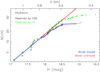 |
Fig. 25 Best-fit solution of the complete Hobson population to the magnitude limit H2 = 19 and its comparison to the observed population. The single power law ℳl model with the free parameter representing the slope γ. The best fit value is γ = 0.81, and the corresponding |


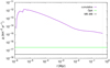 |
Fig. 26 Intrinsic collisional probability |


 |
Fig. 27 Initial and final size distribution of the asteroid main belt (blue) and the synthetic Datura family (cyan) from the 500 kyr lasting simulation of the Boulder code. Intrinsic collisonal probabilities and impact velocities as described in the text. The observed Datura family population from Table A.1 shown by the black curve. No evolution is seen in both populations over the tested timescale and for the sizes displayed. |
Acknowledgements
We thank the referee for very useful suggestions on the submitted version of the paper. We are grateful to the Catalina Sky Survey staff, Eric Christensen and Franck Shelly in particular, for providing us the CSS observations in between 2013 and 2022 in a user-friendly format and allowing us to use them for this research. This work was supported by the Czech Science Foundation (grant 21-11058S).
Appendix A Members of the very young families
Here we provide an information about membership in the very young asteroid families studied in this paper. Our approach to obtain these results is based on two criteria. First, we search for asteroids located in the vicinity of the largest member in the 5D space of osculating orbital elements (disregarding longitude in orbit λ): semimajor axis a, eccentricity e, inclination I, longitude of node Ω, and argument of perihelion ω. Unlike in Nesvorný & Vokrouhlický (2006), we do not use any specific metric function, but simply select all asteroids with orbits in a certain box. In particular, we let the orbital elements vary by the following limits: (i) semimajor axis by ±0.03 au, (ii) eccentricity by ±0.03, (iii) inclination by ±0.2°, and (iv) longitude of node and argument of perihelion both by ±30°. These values are larger than the short-period oscillations of these elements due to planetary perturbations, and conservative enough to sense the population even to the smallest currently detectable sizes (note that small members might have been ejected with larger velocity than the larger ones, constituting the family core). Given the large increase in number of discovered asteroids, there is a small but nonzero chance that such a simple selection method may associate background (unrelated) objects to the family even in the vast 5D space. For that reason, we perform in the second step a convergence control. We numerically integrate orbits of all identified asteroids backward in time for 2 Myr. To keep things simple, we use only nominal (best-fit) initial data at MJD epoch 60,000.0 and include only gravitational perturbations from all planets (disregarding thermal accelerations).12 The planetary configuration at the initial epoch is obtained from the JPL ephemerides file DE 421. As a result, the purpose of this simulation is not to accurately determine the age of the family, which is for most cases known from previous studies, but to eliminate possible interloping objects. We found that the secular angles in the interloper cases show a rapid divergence from the largest body in the family and may be easily identified. Obviously, we eliminated these objects from our analysis of the size distribution of the family members. There was only a limited amount of such objects found. The most crowded situation occurred for Datura family, where we eliminated 80 such objects, i.e., little less than the family members (who are strongly clustered in the simple 5D box of orbital elements that we considered for family-member search).
Datura family as of June 2023.
Adelaide family as of June 2023.
Hobson family as of June 2023.
Rampo family as of June 2023.
Wasserburg family as of June 2023.
Martes family as of June 2023.
Lucascavin family as of June 2023.
References
- Asphaug, E., Collins, G., & Jutzi, M. 2015, in Asteroids IV, eds. P. Michel, F. E. DeMeo, & W. F. Bottke, 661 [Google Scholar]
- Bottke, W. F., Brož, M., O’Brien, D. P., et al. 2015a, in Asteroids IV, eds. P. Michel, F. E. DeMeo, & W. F. Bottke, 701 [Google Scholar]
- Bottke, W. F., Vokrouhlický, D., Walsh, K. J., et al. 2015b, Icarus, 247, 191 [CrossRef] [Google Scholar]
- Bottke, W. F., Vokrouhlický, D., Ballouz, R. L., et al. 2020, AJ, 160, 14 [Google Scholar]
- Carruba, V., Ramos, L. G. M., & Spoto, F. 2020, MNRAS, 493, 2556 [NASA ADS] [CrossRef] [Google Scholar]
- Christensen, E., Africano, B., Farneth, G., et al. 2019, in EPSC-DPS Joint Meeting 2019, EPSC-DPS2019-1912 [Google Scholar]
- Dahlgren, M. 1998, A&A, 336, 1056 [NASA ADS] [Google Scholar]
- Durda, D. D., Bottke, W. F., Nesvorný, D., et al. 2007, Icarus, 186, 498 [NASA ADS] [CrossRef] [Google Scholar]
- Greenberg, R. 1982, AJ, 87, 184 [Google Scholar]
- Hirayama, K. 1918, AJ, 31, 185 [Google Scholar]
- Jacobson, S. A., & Scheeres, D. J. 2011, Icarus, 214, 161 [CrossRef] [Google Scholar]
- Jutzi, M., Holsapple, K., Wunneman, K., & Michel, P. 2015, in Asteroids IV, eds. P. Michel, F. E. DeMeo, & W. F. Bottke, 679 [Google Scholar]
- Marzari, F., Scholl, H., & Farinella, P. 1996, Icarus, 119, 192 [NASA ADS] [CrossRef] [Google Scholar]
- Masiero, J. R., Mainzer, A. K., Grav, T., et al. 2011, ApJ, 741, 68 [Google Scholar]
- Masiero, J. R., DeMeo, F. E., Kasuga, T., & Parker, A. H. 2015, in Asteroids IV, eds. P. Michel, F. E. DeMeo, & W. F. Bottke, 323 [Google Scholar]
- Melosh, H. J. 1989, Impact Cratering: A Geologic Process (Oxford: Oxford University Press) [Google Scholar]
- Michel, P., Richardson, D. C., Durda, D. D., Jutzi, M., & Asphaug, E. 2015, in Asteroids IV, eds. P. Michel, F. E. DeMeo, & W. F. Bottke, 341 [Google Scholar]
- Migliorini, F., Zappalà, V., Vio, R., & Cellino, A. 1995, Icarus, 118, 271 [NASA ADS] [CrossRef] [Google Scholar]
- Morbidelli, A., Bottke, W. F., Nesvorný, D., & Levison, H. F. 2009, Icarus, 204, 558 [Google Scholar]
- Mothé-Diniz, T., & Nesvorný, D. 2008, A&A, 486, L9 [NASA ADS] [CrossRef] [EDP Sciences] [Google Scholar]
- Nesvorný, D., & Vokrouhlický, D. 2006, AJ, 132, 1950 [Google Scholar]
- Nesvorný, D., Vokrouhlický, D., & Bottke, W. F. 2006, Science, 312, 1490 [Google Scholar]
- Nesvorný, D., Brož, M., & Carruba, V. 2015, in Asteroids IV, eds. P. Michel, F. E. DeMeo, & W. F. Bottke, 297 [Google Scholar]
- Nesvorný, D., Vokrouhlický, D., Shelly, F., et al. 2023, Icarus, submitted [Google Scholar]
- Novakovic, B., & Radovic, V. 2019, RNAAS, 3, 105 [NASA ADS] [Google Scholar]
- Novakovic, B., Vokrouhlický, D., Spoto, F., & Nesvorný, D. 2022, Celest. Mech. Dyn. Astron., 134, 34 [NASA ADS] [CrossRef] [Google Scholar]
- Öpik, E. J. 1951, Proc. R. Irish Acad. Sect. A, 54, 165 [Google Scholar]
- Polishook, D., Moskovitz, N., Binzel, R. P., et al. 2014, Icarus, 233, 9 [NASA ADS] [CrossRef] [Google Scholar]
- Pravec, P., & Vokrouhlický, D. 2009, Icarus, 204, 580 [NASA ADS] [CrossRef] [Google Scholar]
- Pravec, P., Vokrouhlický, D., Polishook, D., et al. 2010, Nature, 466, 1085 [NASA ADS] [CrossRef] [Google Scholar]
- Pravec, P., Fatka, P., Vokrouhlický, D., et al. 2018, Icarus, 304, 110 [Google Scholar]
- Pravec, P., Fatka, P., Vokrouhlický, D., et al. 2019, Icarus, 333, 429 [NASA ADS] [CrossRef] [Google Scholar]
- Press, W. H., Teukolsky, S. A., Vetterling, W. T., & Flannery, B. P. 2007, Numerical Recipes: The Art of Scientific Computing (Cambridge: Cambridge University Press) [Google Scholar]
- Rosaev, A., & Plávalová, E. 2016, ArXiv e-prints [arXiv:1612.04951] [Google Scholar]
- Rosaev, A., & Plávalová, E. 2017, Planet. Space Sci., 140, 21 [NASA ADS] [CrossRef] [Google Scholar]
- Rosaev, A., & Plávalová, E. 2018, Icarus, 304, 135 [Google Scholar]
- Schwamb, M. E., Jones, R. L., Yoachim, P., et al. 2023, ApJS, 266, 22 [NASA ADS] [CrossRef] [Google Scholar]
- Spoto, F., Milani, A., & Kneževic, Z. 2015, Icarus, 257, 275 [NASA ADS] [CrossRef] [Google Scholar]
- Tricarico, P. 2017, Icarus, 284, 416 [NASA ADS] [CrossRef] [Google Scholar]
- Vernazza, P., Binzel, R. P., Rossi, A., Fulchignoni, M., & Birlan, M. 2009, Nature, 458, 993 [NASA ADS] [CrossRef] [Google Scholar]
- Vernazza, P., Brož, M., Drouard, A., et al. 2018, A&A, 618, A154 [NASA ADS] [CrossRef] [EDP Sciences] [Google Scholar]
- Vokrouhlický, D. & Nesvorný, D. 2008, AJ, 136, 280 [CrossRef] [Google Scholar]
- Vokrouhlický, D., Brož, M., Bottke, W. F., Nesvorný, D., & Morbidelli, A. 2006, Icarus, 182, 118 [Google Scholar]
- Vokrouhlický, D., Nesvorný, D., & Bottke, W. F. 2008, ApJ, 672, 696 [Google Scholar]
- Vokrouhlický, D., Durech, J., Michalowski, T., et al. 2009, A&A, 507, 495 [NASA ADS] [CrossRef] [EDP Sciences] [Google Scholar]
- Vokrouhlický, D., Durech, J., Polishook, D., et al. 2011, AJ, 142, 159 [CrossRef] [Google Scholar]
- Vokrouhlický, D., Pravec, P., Durech, J., et al. 2017a, A&A, 598, A91 [Google Scholar]
- Vokrouhlický, D., Pravec, P., Durech, J., et al. 2017b, AJ, 153, 270 [CrossRef] [Google Scholar]
- Vokrouhlický, D., Brož, M., Novakovic, B., & Nesvorný, D. 2021a, A&A, 654, A75 [NASA ADS] [CrossRef] [EDP Sciences] [Google Scholar]
- Vokrouhlický, D., Novakovic, B., & Nesvorný, D. 2021b, A&A, 649, A115 [NASA ADS] [CrossRef] [EDP Sciences] [Google Scholar]
- Wetherill, G. W. 1967, J. Geophys. Res., 72, 2429 [Google Scholar]
The first attempt of the method has been carried out by Vokrouhlický et al. (2017a), who applied it to the case of Datura family. However, both (i) the precise detection efficiency characterization of the older set of Catalina survey observations, and (ii) mainly the Datura family known population, were significantly smaller than in the present paper.
We used 10 000 synthetic orbits characteristic to the family and λ uniformly distributed in its definition interval to determine the mean value of p(H).
Obviously, a second criterion of their selection is that CSS detected a significant fraction of known members in these families during its phase 2 operations.
All three of them were pre-covered on CCD images taken by Pan-STARRS in 2011, and also detected in 2014 by a 4-m Victor M. Blanco telescope on Cerro Tololo, using the Dark Energy Camera, which can reach much fainter objects than the 1.5-m G96 telescope.
The smaller members, (180255) 2003 VM9 and (209570) 2004 XL40, were detected only 1 and 4 times during the phase 1, though.
In fact, (6070) Rheinland has been detected 8 and 26 times during the phases 1 and 2, while (54827) Kurpfalz has been detected 8 and 21 times the phases 1 and 2.
Results discussed in this section do not include (429988) 2013 PZ36 among the family members. However, our tests showed that they are robust. By including this body, we observe only a statistically insignificant change of the solution, the largest for  parameter of the ℳ2 model.
Taken very naively, namely just multiplying dimensions of the box in all searched orbital elements, the “volume” of the Box 4 is ≃2.3 larger than that of the Box 3. The number of background asteroids increased by a factor of 56/26 ≃ 2.15. This may indicate roughly uniform, but very sparse, population of background population at the location of the Adelaide family.
We found it interesting to present some details of this numerical experiment, since we are not aware of a similar work previously published. It might be used as a template for studies of other very young families in the future.
We use a well-tested and publicly available integration package swift (http://www.boulder.swri.edu/~hal/swift.html) with a short timestep of 2 d. We output the asteroid heliocentric state vectors every 5 yr and monitor convergence of the secular angles Ω and ϖ toward the reference values of the largest member in the family.
All Tables
All Figures
|
Fig. 1 Osculating values of the secular angles – longitude of node Ω (abscissa) and longitude of perihelion ϖ (ordinate) – for members in the Datura family (epoch MJD 60 000.0). The black symbols show multi-opposition orbits, gray symbols are for the singleopposition orbits; diamond symbol for (1270) Datura, the largest member. Larger/smaller relative values of the secular angles, measured with respect to (1270) Datura, are correlated with positive/negative shift in proper semimajor axis ∆aP (as explained by the arrows). Because the node drifts in a retrograde sense, while the perihelion drifts in the prograde sense, their trends are opposite to each other (thence anticorrelation of the two angles). Location of the exterior mean motion resonance M9/16 with Mars is mapped where the label shows. The dashed line with a slope −0.5 indicates the (anti-) correlation trend. The symbol indicated by a question mark shows projection of (429988) 2013 PZ36 (an object captured on a very chaotic orbit possibly in the exterior mean motion resonance E3/10 with Earth), whose association to the Datura family is uncertain. |
| In the text | |
|
Fig. 2 Top panel: cumulative magnitude distribution N(< H) of the Datura family members. The black symbols are all 91 known members (including the largest asteroid (1270) Datura shown by the diamond, but disregarding (429988) 2013 PZ36, whose membership in the family is uncertain); the red symbols are 60 members detected by CSS during the phase 2 operations. The top abscissa indicates an approximate size computed from H with an assumption of pv = 0.24 value of the geometric albedo. Bottom panel: detection probability p(H) of Datura members as a function of H during the phase 2 operations of CSS based on analysis of geometric and photometric detection factors ran on a large synthetic population of Datura members. We find that p = 1 up to H ≃ 18 magnitude, which sets the limit where the Datura population is complete (dashed line on the upper panel). Beyond this limit p decreases to zero at about 21 magnitude. |
| In the text | |
|
Fig. 3 Number of detections of the identified Datura family members during the phase 2 CSS operations: the largest body (1270) Datura shown by a diamond symbol and highlighted using a label, other 59 smaller members shown by black symbols. The red line is the theoretical prediction based on a large synthetic Datura population computed together with the detection probability p(H) from Fig. 2. The blue curve is a mean number of detections for the observed Datura members computed on a running window of 7 consecutive data-points. |
| In the text | |
|
Fig. 4 Osculating values of the secular angles – longitude of node Ω (abscissa) and longitude of perihelion ϖ (ordinate) – for members in the Adelaide family (epoch MJD 60 000.0). The black symbols show multiopposition orbits, gray symbols are for the singleopposition orbits; diamond symbol for (525) Adelaide, the largest member. The dashed line has the expected slope −0.5 (see, e.g., Figs. 1 and 9 for Datura and Rampo families), but the data are more scattered in the Adelaide case. This is likely due to Mars perturbation discussed in Vokrouhlický et al. (2021b). |
| In the text | |
|
Fig. 5 Top panel: cumulative magnitude distribution N(< H) of the Adelaide family members. The black symbols are all 79 known members (including the largest asteroid (535) Adelaide shown by the diamond), the red symbols are 63 members detected by CSS during the phase 2 operations. The top abscissa indicates an approximate size computed from H with an assumption of pV = 0.24 value of the geometric albedo. Bottom panel: detection probability p(H) of Adelaide members as a function of H during the phase 2 operations of CSS based on analysis of geometric and photometric detection factors ran on a large synthetic population of Adelaide members. We find that p = 1 up to H ≃ 18.2 magnitude, which sets the limit where the Adelaide population is complete (dashed line on the upper panel). Beyond this limit p decreases to zero at about 20.4 magnitude. |
| In the text | |
|
Fig. 6 Number of detections of the identified Adelaide family members during the phase 2 CSS operations: the largest body (525) Adelaide shown by a diamond symbol and highlighted using a label, other 62 smaller members shown by black symbols. The red line is the theoretical prediction based on a large synthetic Adelaide population computed together with the detection probability p(H) from Fig. 5. The blue curve is a mean number of detections for the observed Adelaide members computed on a running window of 9 consecutive data-points. |
| In the text | |
|
Fig. 7 Top panel: cumulative magnitude distribution N(< H) of the Hobson family members. The black symbols are all 60 known members (including the largest asteroids (18777) Hobson and (57738) 2001 UZ160 shown by the diamond), the red symbols are 33 members detected by CSS during the phase 2 operations. The top abscissa indicates an approximate size computed from H with an assumption of pV = 0.2 value of the geometric albedo. Bottom panel: detection probability p(H) of Hobson members as a function of H during the phase 2 operations of CSS based on analysis of geometric and photometric detection factors ran on a large synthetic population of Hobson members. We find that p = 1 up to H ≃ 17.2 magnitude, which sets the limit where the Hobson population is complete (dashed line on the upper panel). Beyond this limit p decreases to zero at about 19.5 magnitude. |
| In the text | |
|
Fig. 8 Number of detections of the identified Hobson family members during the phase 2 CSS operations: the largest bodies (18777) Hobson and (57738) 2001 UZ160 shown by a diamond symbol and highlighted using a label, other 31 smaller members shown by black symbols. The red line is the theoretical prediction based on a large synthetic Hobson population computed together with the detection probability p(H) from Fig. 7. The blue curve is a mean number of detections for the observed Hobson members computed on a running window of 9 consecutive data-points. |
| In the text | |
|
Fig. 9 Osculating values of the secular angles – longitude of node Ω (abscissa) and longitude of perihelion ϖ (ordinate) – for members in the Rampo family (epoch MJD 60 000.0). The black symbols show multiopposition orbits, gray symbols are for the singleopposition orbits; diamond symbol for (10321) Rampo, the largest member. Larger/smaller relative values of the secular angles, measured with respect to (10321) Rampo, correlated with positive/negative shift in proper semimajor axis. The node/perihelion trends are opposite, because the node drift in a retrograde sense, while the perihelion drifts in the prograde sense. The dashed line with a slope −0.5 indicates the correlation trend. |
| In the text | |
|
Fig. 10 Top panel: cumulative magnitude distribution N(< H) of the Rampo family members. The black symbols are all 42 known members (including the largest asteroid (10321) Rampo shown by the diamond), the red symbols are 26 members detected by CSS during the phase 2 operations. The top abscissa indicates an approximate size computed from H with an assumption of pV = 0.24 value of the geometric albedo. Bottom panel: detection probability p(H) of Rampo members as a function of H during the phase 2 operations of CSS based on analysis of geometric and photometric detection factors ran on a large synthetic population of Rampo members. We find that p = 1 up to H ≃ 18 magnitude, which sets the limit where the Rampo population is complete (dashed line on the upper panel). Beyond this limit p decreases to zero at about 20 magnitude. |
| In the text | |
|
Fig. 11 Number of detections of the identified Rampo family members during the phase 2 CSS operations: the largest body (10321) Rampo shown by a diamond symbol and highlighted using a label, other 25 smaller members shown by black symbols. The red line is the theoretical prediction based on a large synthetic Rampo population computed together with the detection probability p(H) from Fig. 10. The blue curve is a mean number of detections for the observed Rampo members computed on a running window of 9 consecutive data-points. |
| In the text | |
|
Fig. 12 Top panel: cumulative magnitude distribution N(< H) of the Wasserburg family members. The black symbols are all 8 known members (including the largest asteroid (4765) Wasserburg shown by the diamond), the blue symbols provide the simplest variant of the debiased population. This was obtained by incrementing the population by 1/p(Hi+1), when stepping from absolute magnitude Hi to Hi+1 (i = 1,…,Nobs); the observed (biased) population increments by one by definition. The gray line is an approximate local power-law representation N(< H) ∝ 10γH near H ≃ 19 with γ ≃ 1.4. The top abscissa indicates an approximate size computed from H with an assumption of pV = 0.3 value of the geometric albedo. Bottom panel: Detection probability p(H) of Wasserburg members as a function of H during the phase 2 operations of CSS based on analysis of geometric and photometric detection factors run on a large synthetic population of Wasserburg members. We find that p = 1 up to H ≃ 18.3 magnitude, which sets the limit where the Wasserburg population is complete (dashed line on the upper panel). Beyond this limit p decreases to zero at about 20.5 magnitude. |
| In the text | |
|
Fig. 13 Top panel: cumulative magnitude distribution N(< H) of the Martes family members. The black symbols are all 6 known members (including the largest asteroid (5026) Martes shown by the diamond). The top abscissa indicates an approximate size computed from H with an assumption of pV = 0.06 value of the geometric albedo (conforming the Ch-class taxonomy). Bottom panel: detection probability p(H) of Martes members as a function of H during the phase 2 operations of CSS based on analysis of geometric and photometric detection factors run on a large synthetic population of Martes members. We find that p = 1 up to H ≃ 17.5 magnitude, which sets the limit where the Martes population is complete (dashed line on the upper panel). Beyond this limit p decreases to zero at about 20.5 magnitude. At magnitude ≃20 p ≃ 0.1. This implies that the three very small members recently detected must represent a tiny sample of a much larger population having about the same size. |
| In the text | |
|
Fig. 14 Detection probability of an additional small fragment in the Lucascavin family: (i) the blue curve is p1 during the phase 1 of CSS operations, and (ii) the red curve is p2 during the phase 2 of CSS operations. The black curve is the combined probability p during both phases (Eq. (1)). The gray area allows the existence of an additional small body in the system, whose maximum probability of occurrence is complementary value to the probability p on the left ordinate. |
| In the text | |
|
Fig. 15 Detection probability of a companion to Rheinland and Kurpfalz on their heliocentric orbit: (i) the blue curve is p1 during the phase 1 of CSS operations, and (ii) the red curve is p2 during the phase 2 of CSS operations. The black curve is the combined probability p during both phases (Eq. (1)). The gray area allows the existence of an additional small body in the system, whose maximum probability of occurrence is complementary value to the probability p on the left ordinate. |
| In the text | |
|
Fig. 16 Best-fit solution of the complete Datura population to the magnitude limit H2 = 20 and its comparison to the observed population. Left panel: the single power law ℳl model with the free parameter representing the slope γ. The best fit value is γ = 0.70, and the corresponding |
| In the text | |
|
Fig. 17 Admissible parameter values of the ℳ2 broken power-law model approximating Datura family absolute magnitude distribution in the range H e (H1, H2) = (18.09, 20). There are three solved-for parameters in the model: (i) the break-point magnitude Hbreak, (ii) the power-law exponent γ1 for H ≤ Hbreak, and (iii) the power-law exponent γ2 for H ≥ Hbreak. Each of the panels shows a projection of the solution onto different 2D subspaces of the 3D space of parameters (Hbreak,γ1,γ2). The dashed line delimits 99% confidence limit zone of the solution, and the gray-scale is proportional to the probability density distribution of the solutions. The best-fit parameter combination is shown by red star symbol. The gray histograms are simply 1D probability density distributions for each of the parameters on the abscissa. The dotted line at γ1 or γ2 values of 0.6 is shown for reference. |
| In the text | |
|
Fig. 18 Probability density distribution of the ratio mftag/mLF (normalized to unit at maximum), where mfrag is the mass/volume of all members up to absolute magnitude 20 without (1270) Datura, and mLF is the mass/volume of the largest member (1270) Datura. Solution using the broken power-law model ℳ2. |
| In the text | |
|
Fig. 19 Best-fit solution of the complete Adelaide population to the magnitude limit H = 20 and its comparison to the observed population. Left panel: the broken power-law model ℳ2 with three adjustable parameters (Hbreak, γ1, γ2). The best-fit values (red star in Fig. 20) are: Hbreak = 18.78, γ1 = 2.08, and γ2 = 0.47, and the corresponding |
| In the text | |
|
Fig. 20 Admissible parameter values of a ℳ2 broken power-law model approximating Adelaide family absolute magnitude distribution in the range H ∈ (H1, H2) = (18.2, 20). There are three solved-for parameters in the model: (i) the break-point magnitude Hbreak, (ii) the power-law exponent γ1 for H ≤ Hbreak, and (iii) the power-law exponent γ2 for H ≥ Hbreak. Each of the panels shows a projection of the solution onto different 2D subspaces of the 3D space of parameters (Hbreak, γ1, γ2). The dashed line delimits 99% confidence limit zone of the solution, and the gray-scale is proportional to the probability density distribution of the solutions. The best-fit parameter combination is shown by red star symbol. The gray histograms are simply 1D probability density distributions for each of the parameters on the abscissa; the dashed histograms along the distributions of the γ1 and γ2 exponents correspond to the first and the last exponent in the ℳ3 broken power-low models with two break-points (Hbreak,1, Hbreak,2; i.e., the first in the interval (18.2, Hbrκak,1), and the second in the interval (Hbreak,2, 20)). The dotted line at γ1 or γ2 values of 0.6 is shown for reference. |
| In the text | |
|
Fig. 21 Probability density distribution of the ratio mfrag/mLF (normalized to unit at maximum), where mfrag is the mass/volume of all members up to absolute magnitude 20 without (525) Adelaide, and mLF is the mass/volume of the largest asteroid (525) Adelaide. The solid/gray histogram for the ℳ2 model, the dashed histogram for the ℳ3 model (all models whose parameters p are within the 99% confidence level of the family population were used). |
| In the text | |
|
Fig. 22 Best-fit solution of the complete Rampo population to the magnitude limit H2 = 20 and its comparison to the observed population. Left panel: the single power law ℳl model with the free parameter representing the slope γ. The best fit value is γ ≃ 1.17, and the corresponding |
| In the text | |
|
Fig. 23 Admissible parameter values of the ℳ2 broken power-law model approximating Rampo family absolute magnitude distribution in the range H ∊ (H1, H2) = (18.1, 20). There are three solved-for parameters in the model: (i) the break-point magnitude Hbreak, (ii) the power-law exponent γ1 for H ≤ Hbreak, and (iii) the power-law exponent γ2 for H ≥ Hbreak. Each of the panels shows a projection of the solution onto different 2D subspaces of the 3D space of parameters (Hbreak, γ1, γ2) The dashed line delimits 99% confidence limit zone of the solution, and the gray-scale is proportional to the probability density distribution of the solutions. The best-fit parameter combination is shown by red star symbol. The gray histograms are simply 1D probability density distributions for each of the parameters on the abscissa. The dotted line at γ1, or γ2 values of 0.6 is shown for reference. |
| In the text | |
|
Fig. 24 Probability density distribution of the ratio mfrag/mLF (normalized to unit at maximum), where mfrag is the mass/volume of all members up to absolute magnitude 20 without (10321) Rampo, and mLF is the mass/volume of the largest asteroid (10321) Rampo. Solution using the broken power-law model ℳ2. |
| In the text | |
|
Fig. 25 Best-fit solution of the complete Hobson population to the magnitude limit H2 = 19 and its comparison to the observed population. The single power law ℳl model with the free parameter representing the slope γ. The best fit value is γ = 0.81, and the corresponding |
| In the text | |
|
Fig. 26 Intrinsic collisional probability |
| In the text | |
|
Fig. 27 Initial and final size distribution of the asteroid main belt (blue) and the synthetic Datura family (cyan) from the 500 kyr lasting simulation of the Boulder code. Intrinsic collisonal probabilities and impact velocities as described in the text. The observed Datura family population from Table A.1 shown by the black curve. No evolution is seen in both populations over the tested timescale and for the sizes displayed. |
| In the text | |
Current usage metrics show cumulative count of Article Views (full-text article views including HTML views, PDF and ePub downloads, according to the available data) and Abstracts Views on Vision4Press platform.
Data correspond to usage on the plateform after 2015. The current usage metrics is available 48-96 hours after online publication and is updated daily on week days.
Initial download of the metrics may take a while.