| Issue |
A&A
Volume 681, January 2024
|
|
|---|---|---|
| Article Number | A75 | |
| Number of page(s) | 9 | |
| Section | Astrophysical processes | |
| DOI | https://doi.org/10.1051/0004-6361/202347241 | |
| Published online | 18 January 2024 | |
Tayler–Spruit dynamo simulations for the modeling of radiative stellar layers
1
LERMA, Observatoire de Paris, PSL Research University, CNRS, Sorbonne Université,
Paris,
France
e-mail: This email address is being protected from spambots. You need JavaScript enabled to view it.
2
Université Côte d’Azur, Inria, CNRS, LJAD,
France
e-mail: This email address is being protected from spambots. You need JavaScript enabled to view it.
3
LPENS, Laboratoire de Physique de l’École Normale Supérieure, ENS, Université PSL, CNRS, Institut Universitaire de France,
Paris,
France
e-mail: This email address is being protected from spambots. You need JavaScript enabled to view it.
4
LPENS Laboratoire de Physique de l’École Normale Supérieure, ENS, Université PSL, CNRS,
Paris,
France
Received:
20
June
2023
Accepted:
18
October
2023
Abstract
Context. Maxwell stresses exerted by dynamo-generated magnetic fields have been proposed as an efficient mechanism to transport angular momentum in radiative stellar layers. Numerical simulations are still needed to understand its trigger conditions and the saturation mechanisms.
Aims. The present study follows up on a recent paper where we reported on the first simulations of Tayler-Spruit dynamos. Here we extend the parameter space explored to assess in particular the influence of stratification on the dynamo solutions. We also present numerical verification of theoretical assumptions made previously that were instrumental in deriving the classical prescription for angular momentum transport implemented in stellar evolution codes.
Methods. A simplified radiative layer is modeled numerically by considering the dynamics of a stably stratified, differentially rotating, magnetized fluid in a spherical shell.
Results. Our simulations display a diversity of magnetic field topologies and amplitudes depending on the flow parameters, including hemispherical solutions. The Tayler-Spruit dynamos reported here are found to satisfy magnetostrophic equilibrium and achieve efficient turbulent transport of angular momentum, following Spruit’s heuristic prediction.
Key words: instabilities / dynamo / stars: kinematics and dynamics / turbulence / magnetic fields / magnetohydrodynamics (MHD)
© The Authors 2024
 Open Access article, published by EDP Sciences, under the terms of the Creative Commons Attribution License (https://creativecommons.org/licenses/by/4.0), which permits unrestricted use, distribution, and reproduction in any medium, provided the original work is properly cited.
This article is published in open access under the Subscribe to Open model. This email address is being protected from spambots. You need JavaScript enabled to view it. to support open access publication.
1 Introduction
Understanding the transport of angular momentum (AM) and chemical elements in stellar interiors is a cornerstone of stellar evolution models (Maeder & Meynet 2000). In recent years, asteroseismic data from space-born missions, namely the CoRoT (Baglin et al. 2009), Kepler, and TESS (Borucki et al. 2010; Aguirre et al. 2020; Rauer et al. 2014) missions, have provided unprecedented insight into the dynamics of internal layers by constraining the rotation rates of the envelope and core of thousands of stars (Aerts et al. 2019). In particular, these observations show that considerable spin-down occurs in the radiative cores of evolved stars through a process that is not explained by current stellar evolution models (Ceillier et al. 2013; Christophe et al. 2018; Van Reeth et al. 2018; Eggenberger et al. 2019; Bugnet 2020).
While AM transport is expected to be influenced by a diversity of physical mechanisms, including stellar winds, contraction and dilatation, meridional circulation, internal gravity waves, and magnetic fields, the last in particular are thought to play a major role as their parameterization in stellar codes has been shown to strongly suppress differential rotation (Eggenberger et al. 2005). However, while surface magnetic fields have been detected in the radiative envelopes of many massive and intermediate-mass stars (Wade et al. 2016), magnetic fields in the radiative cores of post-MS stars are still notoriously difficult to constrain despite the promising detection of magnetic signatures on rotational splittings (Prat et al. 2020; Van Beeck et al. 2020; Mathis et al. 2021). Therefore, the parameterization of magnetically driven AM transport in 1D stellar codes relies on theoretical predictions and on direct numerical simulations to characterize magnetic fields and the condition for their generation in radiative layers.
Magnetic fields can be generated and sustained against ohmic dissipation in the star internal layers through a dynamo instability, whereby a fraction of the kinetic energy of plasma motions is converted into magnetic energy. In radiative zones however, the mechanisms for dynamo action are poorly understood due to the scarcity of numerical simulations. So far, the only theoretical models for radiative dynamo that have been parameterized in stellar codes are driven by magneto-rotational instability (MRI) and Tayler instability (Wheeler et al. 2015; Griffiths et al. 2022). These parameterizations have shown that, while MRI is found to strongly enhance chemical mixing, the most efficient at transporting AM is arguably the Tayler–Spruit dynamo mechanism put forward by Spruit (2002; see also Eggenberger et al. 2022).
In this model, dynamo action results from a constructive feedback loop between the winding up of poloidal magnetic fields into toroidal fields by differential rotation (the Ω-effect) on the one hand, and a strong toroidal magnetic field becoming unstable to a pinch-type instability (Tayler 1973) on the other hand. In Spruit (2002), a scenario for magnetic field amplification is suggested, where differential rotation generates a strong, axisymmetric toroidal field out of an arbitrarily weak poloidal magnetic field, until the former breaks into nonaxisymmetric modes upon reaching a critical amplitude, thus initiating the dynamo loop. This scenario however was never reproduced in numerical simulations despite numerous attempts, so that the possibility for Tayler–Spruit dynamos to operate in radiative stellar layers had remained somewhat controversial (Zahn et al. 2007). Moreover, even assuming that the classical Tayler–Spruit mechanism is indeed relevant for radiative zones, the rotation rates of subgiant stars was shown to remain unaccounted for (Cantiello et al. 2014; Salmon et al. 2022), motivating investigation of alternative, possibly more efficient saturation mechanisms for this dynamo (Fuller et al. 2019). In a forthcoming paper (Daniel et al. 2023), we report that the turbulence induced by the dynamo discussed here produces an additional contribution to angular momentum transport via the Reynolds stress tensor. This could significantly affect the profile of rotation, as for some RGB we show that it could be up to one order of magnitude more important than the magnetic torque applied on the flow.
In a recent paper (Petitdemange et al. 2023), we reported the first numerical evidence of such dynamo solutions in simulated radiative layers of stars. The initialization of the dynamo loop was found to somewhat differ from the original prediction of Spruit (2002), in that the excitation of the Tayler–Spruit dynamo was nonlinearly achieved through the prior excitation of a weaker, shear-driven dynamo instability. Extensive numerical simulations are still needed to fully understand its trigger conditions and the saturation mechanisms, and the first aim of the present paper is to clarify the dominant balances at play in the simulated Tayler–Spruit dynamos at steady state. We then extend our exploration of the parameter space, and report the existence of various dynamo topologies, depending on the stratification regime, and in particular the corresponding hydrodynamic configuration of the base flow.
2 Methods
Our numerical model is presented in detail in the supplementary material of Petitdemange et al. (2023); we briefly recall it here for clarity. In order to considerably reduce costs, our numerical approach focuses on modeling a star’s radiative (stably stratified) layer, without solving for the complicated couplings with the innermost core regions or the external stellar layers that determine the radial shear profile. Instead, we consider a simple numerical setup where differential rotation in the flow is achieved through entrainment by rigid boundaries. In our model, an electrically conducting fluid with magnetic diffusivity η and molecular viscosity v fills the gap between two spherical shells rotating about a common axis at different speeds, where Ω and Ω + ∆Ω are the angular velocities of the outer and inner spheres, respectively. The calculations are performed in the rotating frame of reference where the outer sphere is at rest. The parameters controlling diffusivities are far from realistic due to computational limitations, but we tend to determine systematic behaviors. In addition, it is important to note that the values of effective diffusivities can be increased by several orders of magnitude in strongly turbulent systems such as the tachocline region.
No-slip boundary conditions are applied on both spheres, along with electrically insulating boundary conditions on the outer sphere, whereas the inner sphere has the same conductivity as the fluid. Stable stratification is achieved inside the fluid by prescribing a positive temperature difference ∆T between the inner and outer shells, whose temperatures are fixed. The aspect ratio between the inner and outer spheres radii χ = ri/ro is set to 0.35 throughout the study. We use the Boussinesq approximation to neglect variations in the fluid density except in the buoyancy term, leading to the following magnetohydrodynamic (MHD) equations:
 (1)
(1)
 (2)
(2)
 (3)
(3)
 (4)
(4)
 (5)
(5)
where v, P, B, and T are respectively the velocity field, pressure field, magnetic field, and temperature field; Θ is the temperature fluctuation accounting for density fluctuations in the buoyancy term, ez the unit vector along the rotation axis, and er the local radial unit vector. The physical properties of the fluid are determined by its magnetic permeability µ0, its mean density ρ, its thermal expansion coefficient a, and its thermal diffusivity κ; 𝑔0 denotes the gravitational acceleration at the outer shell.
In terms of numerical control parameters, the flow regime is entirely described by means of five independent, dimensionless parameters: the Ekman number  quantifying the ratio between viscous force and Coriolis acceleration, the Rayleigh number
  measuring the intensity of thermal forcing (hence the strength of the stratification), the Reynolds number Re = riro∆Ω|v measuring the ratio of inertial to viscous effects, the magnetic Reynolds number Rm = riro∆Ω/η comparing the respective effects of induction and ohmic dissipation, and the Prandtl number Pr = v|κ comparing molecular and thermal diffusivities. It is important to note that the extreme flow regimes found in astrophysical flows remain far beyond the reach of numerical simulations, due to their formidable computational cost. In particular, the Ekman number E is of order E ~ 10−15 in stellar interiors, whereas the most intensive highperformance direct numerical simulations (DNSs) currently only reach E ≳ 10−7 − 10−8 (Schaeffer et al. 2017). Simulations in the strongly stratified regime also require a very high spatial resolution as stratification decreases the size of flow structure in the radial direction, and the timestep must be decreased in order to take into account the possibility of internal gravity waves. Nevertheless, 3D DNSs can now achieve fully turbulent strongly stratified flow regimes, due to the ever-increasing availability of numerical resources. Moreover, our simulations systematically span a large range of parameters in order to determine useful scaling laws.
The numerical resolution chosen is large enough so that physical viscosity always dominates over grid viscosity in our nonideal simulations, and our results are therefore independent of the resolution. All the simulations reported in this study were carried out using the PARODY-JA code (Dormy et al. 1998; Aubert et al. 2008) coupled with the ShTns library (Schaeffer 2013). PARODY-JA uses finite-difference discretization in the radial direction and spherical harmonic decomposition.
The number of radial gridpoints (nr) used in the fluid domain is 288 < nr < 360, and the maximum degree (lmax) and order (mmax) of the spherical harmonic decomposition are 128 < lmax < 198 and 58 < mmax < 128, respectively.
3 Comment on hydrodynamic states
Before turning to the dynamo problem, it is worth briefly considering the geometry of the (purely hydrodynamic) base flow, which depends on the rotation and stratification parameters. Weakly stratified, rapidly rotating flows are dominated by a force balance between Coriolis acceleration and pressure gradient, a situation referred to as the geostrophic equilibrium. This dominant balance results in the flow being (at lowest order) invariant along cylinders coaxial with the rotation axis (Proudman 1956). In spherical Couette flow (and below the shear instability threshold), the fluid located outside the notional tangent cylinder encompassing the inner sphere at the equator is co-rotating with the outer sphere. Inside the tangent cylinder (and far from both the boundaries), the fluid rotates at the rate Ω + ∆Ω/2. The velocity jump across the tangent cylinder is accomodated through a series of nested, free shear layers, known as the Stewartson layers (Stewartson 1966), whose thicknesses scale as powers of the rotation parameter E (see Marcotte et al. 2016, who provide a complete description of this problem). When the shear parameter becomes sufficiently large, destabilization of a Stewartson shear layer results in breaking the flow axisymmetry, while invariance along the rotation axis remains largely preserved.
Strongly stratified, slowly rotating flows, on the other hand, exhibit a spherical geometry due to the leading effect of buoyancy; this corresponds to the typical regime where the shellular approximation is meaningful, or in other words, that the angular velocity can be considered (at leading order) invariant in the horizontal direction (Zahn 1992). The transition in flow geometry depends on the relative importance of stratification and global rotation. However, as shown by Philidet et al. (2019), the critical parameter is not the frequency ratio N/Ω between the buoyancy frequency N = (α𝑔∆T/(ro − ri))1/2 and the global rotation rate Ω, but the quantity  , which is equivalently expressed here as Q = E2Ra/(1 − χ). This numerical result of Philidet et al. (2019) can be retrieved with a simple dimensional analysis of the problem. Balancing Coriolis acceleration and buoyancy in the equatorial plane yields
 (6)
(6)
where uϕ and Θ are typical values for the azimuthal velocity and the thermal perturbation, respectively. In the Boussinesq approximation, we can estimate the thermal perturbation at steady state as
 (7)
(7)
where ur is a typical radial velocity; furthermore, the azimuthal component of Eq. (1) in the equatorial plane provides
 (8)
(8)
Combining Eqs. (6)–(8) yields
 (9)
(9)
This qualitative argument further suggests that the crossover regime corresponds to Q of order unity, which happens to be relevant for example in the case of the solar radiative zone due to the smallness of the Prandtl number Pr (with QSun ~ 1.3).
Figure 1 shows that increasing the stratification (controled by the Rayleigh number Ra) when the rotation parameter E and the thermal Prandtl number Pr are fixed tends to stabilize the non-axisymmetric shear instability, which also develops at decreasing wavenumbers. Unsurprisingly, the stability threshold Rec scales as  , which is equivalent to a Richardson number Ri of order unity (Richardson 1920):
 (10)
(10)
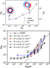 |
Fig. 1 Stratification influence on the onset of shear instability in a spherical shell. Top: evolution of the critical Reynolds number Rec (or equivalently the Rossby number Roc) as a function of stratification intensity (quantified by the Rayleigh number Ra). When Re > Rec (red upward triangles), nonaxisymmetric modes are maintained in time. Conversely, when Re < Rec (dark downward triangles), the kinetic energies of nonaxisymmetric modes exponentially decay with time. The insets highlight the pattern of unstable modes close to the threshold via color maps of the radial velocity in the equatorial plane. Simulations parameters: E = 10−5, Pr = 0.1. Bottom: critical Reynolds number Rec for the onset of hydrodynamic instability with increasing stratification, for various thermal and rotation parameters. |
4 Stratification, rotation, and dynamo morphology: A route to Tayler–Spruit dynamos
The hydrodynamic base states described above are found to power a diversity of self-sustained radiative dynamos, depending on the stratification-to-rotation ratio on the one hand, and on the initial condition for the magnetic field on the other hand. The variety (both in amplitude and in structure) of the dynamo-generated magnetic fields is exemplified by the diagram in Fig. 2, which summarizes the study of the dynamo bifurcation for fixed diffusivity ratios Pr = 0.1, Pm = 1 and rotation parameter E = 10−5, when the Rayleigh number controlling the degree of stratification is varied over four orders of magnitudes. The dynamo morphology can be mainly classified into three categories (see Fig. 3): toroidal, dipolar, and hemispheric dynamos. Toroidal dynamos are characterized here by a strongly dominant axisymmetric toroidal component (representing more than 80% of the magnetic energy), and a largely subdominant, nonaxisymmetric poloidal component dominated by the azimuthal mode m = 1. These dynamos correspond to Tayler–Spruit dynamos (Spruit 2002), numerically reproduced for the first time in Petitdemange et al. (2023) and presented in detail therein. Dipolar dynamos on the other hand refer to dynamos where the poloidal energy only slightly dominates over the toroidal energy, but the former is dominated by the axial dipole. Finally, hemispherical dynamos are characterized by a strong asymmetry between the two hemispheres.
The dipolar dynamos are observed at sufficiently low Ra, where stratification has a minor influence on the MHD flow; these dynamos are similar to those reported in Guervilly & Cardin (2010) without stratification. In this low-Ra regime neither the magnetic field morphology nor its amplitude are found to depend on the initial conditions. The relative weakness of the dynamo-generated magnetic fields results in the flow not being significantly affected by the dynamo: although the total kinetic energy is slightly reduced, the dominant nonaxisymmetric component of the velocity field remains unchanged compared to the purely hydrodynamic simulations.
Stratification effects become nonnegligible as Ra increases to Ra = 108. In Fig. 2 two distinct branches of dynamo solutions can be observed depending on the magnetic seed field prescribed initially. Specifically, tiny random magnetic fields are amplified and evolve toward saturated dipolar dynamos (dashed line with circles), whereas systems initialized with a stronger, well-chosen magnetic field spontaneously evolve toward a new equilibrium, corresponding to a toroidal (Tayler–Spruit) dynamo (dashed line with stars). These two branches appear as soon as Re/Rec becomes slightly greater than one, meaning that both solutions require the hydrodynamic instability to set in for a magnetic field to be maintained by dynamo action. For Re < Rec, the magnetic energy and the kinetic energy of all nonaxisymmetric modes eventually undergo exponential decay whatever the tested initial condition. Moreover, the amplitude of the saturated magnetic field is more than one order of magnitude larger for Tayler–Spruit dynamos than for dipolar dynamos (and almost three orders of magnitude for Re/Rec < 1.5). As a consequence, Tayler–Spruit dynamos are observed to trigger MHD turbulence, whereas dipolar solutions are not. As shown in Petitdemange et al. (2023), the associated transport of angular momentum tends to suppress the shear in the bulk of the flow where magnetic activity is most intense.
The rich dynamo topology of this moderately stratified regime is further illustrated by the emergence of hemispherical dynamo solutions. Figure 3 shows meridional maps of the angular velocity and magnetic fields. In these dynamo solutions, magnetic activity is nearly absent from one hemisphere, and the flow corresponds to that of the hydrodynamic state, with columnar vortices aligned with the tangent cylinder. In the other hemisphere, a strong, large-scale axisymmetric toroidal magnetic field builds up at mid-latitudes. In comparison, the radial component has a typical length scale that is smaller, and it is dominated by its nonaxisymmetric components. The field strength for these dynamos is strong enough to considerably modify the flow structure in the hemisphere influenced by the magnetic field: the cylindrical symmetry of the flow is broken and the nonaxisymmetric components of the radial velocity exhibit the same spatial distribution as the magnetic field.
As Ra further increases, however, a crucial feature of Tayler– Spruit dynamos is that some strong magnetic fields can be maintained, not only below the linear instability threshold for dynamo action, but even below the shear instability threshold (Petitdemange et al. 2023). In the Ra = 109 series presented in Fig. 2 for example, no initially weak magnetic fields are amplified up to Re/Rec ~ 1.75. Above this threshold, initially weak seed fields are amplified by dynamo action and develop into strong, toroidal fields, which in turn promote turbulent fluid motions. We note that all the series shown in this particular figure correspond to Pm = 1. Another type of dynamo, morphologically similar to the Tayler–Spruit dynamos presented here, but considerably weaker and essentially laminar, can be obtained at lower Pm and was reported in Petitdemange et al. (2023). These strong dynamo-generated fields could be maintained down to Re ~ 0.5Rec, modifying the flow so as to sustain the turbulent motions that power them even below the (hydrodynamic) instability threshold. In Daniel et al. (2023), we show by a Pm study that the relevant criterion controlling how low the system can go before losing dynamo action (in terms of differential rotation) is actually a constant magnetic Reynolds number, whose value is fixed by the global rotation and stratification, in very good agreement with what was proposed by Spruit (2002). It is therefore likely that in a real star, as the Rm number is large, Tayler–Spruit dynamos could flatten rotation profiles across the radiative zone and still operate even when the shear becomes comparatively weak.
This subcriticality of the Tayler–Spruit mechanism was certainly instrumental to numerically reproduce these particular dynamo solutions, and may explain why they have long eluded numerical investigation. Tayler–Spruit dynamos here can be obtained from initially weak, random seed fields only when the shear is sufficiently strong and the base flow axisymmetry is broken by the hydrodynamic instability, meaning that  . While this is never a restrictive condition in a (real) stellar interior, where the expected Reynolds numbers are of order Re ~ 1010 or larger, it certainly is restrictive for numerical simulations, for which the computational cost associated with the shear-unstable regime rapidly becomes overwhelming at large Ra (strong stratification). In other words, attempting to grow a numerical Tayler–Spruit dynamo directly out of weak, random magnetic fields using, for example, a solar-like ratio N/Ω ~ 100 and a reasonably small rotation parameter E ≪ 1 is practically impossible. This may seem particularly surprising since Tayler–Spruit’s theory predicts dynamo action out of vanishingly small initial perturbations, due to prior amplification through the Ω-effect; while this scenario may apply in true radiative stellar layers, the required flow regimes might not permit such a scenario in numerical simulations.
In our approach, instead, we exploit the subcriticality of Tayler–Spruit dynamos to reach high N/Ω regimes by first addressing the computationally more accessible supercritical flow regime (Re > Rec) for N/Ω = O(1). Once a dynamo builds up, the resulting magnetic and velocity fields at steady state are used to initialize a new simulation, where the control parameters defining the flow regime are slightly modified. Once the fields have adjusted to the new flow conditions and settled into a steady state, the latter is used to initialize a new simulation where the control parameters are further modified, and so on. Following the dynamo manifold requires that the control parameters vary slowly while exploring the parameter space, due to the subcritical nature of the dynamo. Despite the numerical constraints, we find that Tayler–Spruit dynamos are surprisingly robust and actually span a wide spectrum of flow regimes. While many simulations here are performed with low N/Ω ratios that are relevant for rapid rotators, it was possible to obtain a few simulations with N/Ω up to 20 and 50, thus approaching the solar ratio (N/Ω|Sun ~ 100). These simulations correspond to Q = 62 and Q = 246, respectively, meaning that the base flow has very clear spherical symmetry. The velocity and magnetic maps shown in Fig. 4, both corresponding to Tayler–Spruit simulations, exemplify the clear emergence of this symmetry as Q increases and the robustness of the dynamo mechanism with respect to the flow geometry.
It is important to note that, while our simulations present a few typical properties indicating that a Tayler instability is at work to generate the nonaxisymmetric fluctuations whose nonlinear interactions close the dynamo loop, the possibility for the azimuthal field to become destabilized through azimuthal magnetorotational instability (AMRI) in some parameter regimes, and thus to feed the dynamo cannot be ruled out. For example, simulations by Guseva et al. (2017) have shown that AMRI can drive a dynamo and sustain MHD turbulence in a cylindrical shear flow. Motivated by the design of experiments, the stability of an azimuthal, background magnetic field has been investigated in cylindrical geometry, considering different radial variations of the background magnetic and velocity field (Kirillov et al. 2014; Rüdiger et al. 2018). These studies have shown that purely azimuthal fields can trigger both Tayler instability and AMRI, and that their instability domains actually overlap in some regions of the parameter space, making the distinction between the two mechanisms somewhat difficult. In the present case, several indicators point toward the Tayler instability. As we show in Petitdemange et al. (2023; Fig. 2), the secondary energy growth characterizing the onset of strong, toroidal dynamo action occurs at the time where the local stability criterion for Tayler instability is met, as quantified using the local Elsasser number. Secondly, at high Pm, Daniel et al. (2023) find that the minimum shear rate (controlled by the Rossby number) required to maintain these strong dynamo solutions is in good agreement with the predictive scaling of Spruit (2002). Finally, the radial profile of the corresponding axisymmetric, azimuthal magnetic field is shown in Fig. 5 (top), where the magnetic Rossby number  measures the local steepness of the axisymmetric component of the azimuthal field
  . A comparison with the meridional map of nonaxisymmetric magnetic fluctuations in Fig. 5 (bottom) reveals that the latter develop only when the large-scale field increases sufficiently quickly in radius, as in Spruit’s scenario. More specifically, non-axisymmetric fluctuations take place in the region, relatively close to the inner sphere, where Rb > 0; this is always found to promote Tayler instability in the setups considered by Kirillov et al. (2014). Conversely, the flow domain where Rb < −0.5, which is a priori expected to be prone only to AMRI following Kirillov et al. (2014), remains well off the dynamo active region. Some caution is needed when interpreting the present simulations in light of these studies, which consider unstratified fluids and a different geometry, and it would be desirable to investigate how these results pertain to the stratified case and spherical geometry in a future work.
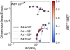 |
Fig. 2 Time-averaged magnetic energy for dynamo simulations performed with different parameters and initial conditions for the magnetic field. The stars correspond to models in which the axisymmetric toroidal magnetic component exceeds 80% of the total magnetic energy (toroidal dynamos). The fixed simulation parameters are E = 10−5, Pr = 0.1, Pm = 1. |
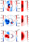 |
Fig. 3 Meridional sections of the axisymmetric components of azimuthal magnetic Bϕ, radial magnetic field Br, and angular velocity Ω⋆ (normalized by ΔΩ). Top: weakly stratified dipolar dynamo at E = 10−5, Ra = 107, Re = 5000, Pr = 0.1, Pm = 1. Middle: hemispherical dynamo at E = 10−5, Ra = 108, Re = 12000, Pr = 0.1, Pm = 1. Bottom: strong toroidal (Tayler–Spruit) dynamo at E = 10−5, Ra = 1010, Re = 3.104, Pr = 0.1, Pm = 1. |
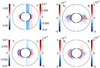 |
Fig. 4 Meridional sections of axisymmetric latitudinal and radial components of the velocity field (left) and magnetic field (right). Parameters: Re = 2.75 × 10⁴ and Ra = 109 (uppel panel; Q = 0.15); Re = 3.104 and Ra = 1010 (lower panel; Q = 1.5). The other control parameters are fixed as in Fig. 3. |
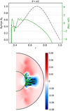 |
Fig. 5 Distribution of axisymmetric and nonaxisymmetric magnetic components. Top: radial profile of the magnetic Rossby number Rb and the axisymmetric azimuthal field |


5 Saturation of the Tayler–Spruit dynamo and angular momentum transport
A major consequence for the possible existence of Tayler–Spruit dynamos in radiative stellar layers is the resulting enhancement of angular momentum (AM) transport. Quantitative prediction of AM transport, however, requires understanding the saturation processes at play in the Tayler–Spruit dynamo loop. In the seminal paper Spruit (2002), the author derives a theoretical prediction for quantifying the azimuthal Maxwell stress T ~ BrBϕ/µ using dimensional analysis. The derivation can be summarized as follows. First, the azimuthal component of the induction equation at steady state provides a balance between the amplification of the azimuthal field by the Ω-effect on the one hand, and its (effective) damping through Ohmic diffusion on the other hand. At leading order,
 (11)
(11)
where lr is the typical radial (vertical) lengthscale for magnetic activity, Br and Bϕ are the typical amplitudes of the radial and azimuthal dynamo-generated field, and ηeff is the effective (i.e., turbulent) magnetic diffusivity. Simple dimensional arguments stemming from mixing length theory suggest that  , where
  is the growth rate of the Tayler instability Spruit (2002), such that
 (12)
(12)
where we follow Spruit’s notation for the dimensionless shear rate q = r∂rΩ/Ω. The typical radial scale for dynamo activity can be chosen as the largest unstable length scale with respect to the Tayler instability:
 (13)
(13)
The scaling above derives from the consideration that stratification suppresses instability at the largest scales, and is obtained for the case κ = 0. A classical way of reinstating thermal diffusivity when κ ≫ η ≠ 0 is to observe, since thermal diffusion acts on a shorter timescale than the dynamo, that its effect is merely to partly suppress temperature gradients, thus decreasing the effective buoyancy frequency  (Zahn 1974).
A last equation is needed to close the system and evaluate T. For this, Spruit (2002) considers the rate at which the radial magnetic field is generated from the axisymmetric azimuthal field by Tayler-unstable displacements to write
 (14)
(14)
Since Bϕ is slowly varying in r, this can be obtained by noting
 (15)
(15)
where τ is the production timescale of Br through the Tayler instability, and ur the radial velocity associated with unstable displacements. Combined together, Eqs. (12)–(14) yield the predictive scaling law for the Maxwell stress in the diffusionless case:
 (16)
(16)
The arguments used to derive Eq. (16) in Spruit (2002) have been largely debated (e.g., Zahn et al. 2007) owing to the fact that the most unstable azimuthal wavenumber with respect to the Tayler instability is not m = 0 but m = 1. As a result, the radial field Br produced in Eq. (15) should be dominated by the m = 1 component, which can hardly (directly) replenish the axisymmetric Bϕ through Ω-effect in Eq. (12). This is not a theoretical obstacle in a turbulent flow, however, since nonlinear interactions between small-scale velocity and magnetic fluctuations can produce the required axisymmetric fields through the mean-field effect (Moffatt 1978). The scaling Eq. (14) could also be recovered using an alternative argument, that Br can only grow through the Tayler instability until the latter is quenched by magnetic tension (Fuller et al. 2019). Further investigation is certainly needed to clarify the complicated saturation mechanisms of the Tayler instability (Ji et al. 2023). However, a sufficient requirement for the AM transport prediction in Eq. (16) to hold is, rather than Eqs. (13) and (14) being independently satisfied, that their combination be true:
 (17)
(17)
Replacing Eq. (17) in the induction equation dominant balance in Eq. (12) is sufficient in order to derive Eq. (16). The scaling law in Eq. (17) turns out to be satisfied in our turbulent Tayler– Spruit dynamo simulations: Fig. 6 (upper panel) shows the ratios Br/Bϕ versus  , as crudely estimated from the time- and volume-averaged magnetic energy contained in the poloidal and toroidal axisymmetric magnetic field components, respectively. Even though both ratios vary by only one order of magnitude throughout all the simulations, the scaling law in Eq. (17) was found to hold over more than two decades in the magnetic field amplitude. It is rather more delicate to accurately assess the robustness of scaling Eq. (13) in our simulations, due to the difficulty of finding an objective (and automatic) criterion to precisely measure the width of the most active dynamo region. Despite this caveat, the typical width is always found to be on the order of 0.1 dimensionless units in our simulations (e.g., Fig. 4), which, given the unknown geometric prefactors in the various scaling laws, is roughly compatible with the magnitude of the ratio
  .
.
Importantly, the Tayler–Spruit dynamo simulations presented here and in Petitdemange et al. (2023) are found to be in good agreement with Eq. (16), as illustrated in Fig. 6 (bottom panel). To test the scaling law against our simulations, we measure the dimensionless magnetic torque
 (18)
(18)
with S(r) the sphere of radius r centered at the origin, in the fluid region of the most intense magnetic activity and compare it with the scaling law
 (19)
(19)
where uϕ is the axisymmetric azimuthal velocity at radius r. The numerical procedure used to calculate Gmag from our simulations is detailed in the Supplementary Material of Petitdemange et al. (2023). The equivalence between Eq. (19) and Spruit’s prediction in Eq. (16) is made possible because we use the following estimate of the dimensionless shear rate q,
 (20)
(20)
which we replace in Eq. (16) to obtain
 (21)
(21)
and thus Eq. (19). One may wonder why q is not constructed instead on the difference in rotation rates between the inner and outer sphere (i.e., the Rossby number):
 (22)
(22)
This is because our modeling choice of differentially rotating rigid boundaries to prescribe a sheared velocity profile across the fluid domain, while numerically convenient, comes with a caveat: most of the shear is accomodated in the (very) thin viscous boundary layer attached to the inner sphere. However, the peak of magnetic field intensity is found well away from the boundary, in a region where viscous effects are negligible. As a result, the shear that is effectively left across the dynamo region is significantly smaller than the total shear q′. It is almost completely accommodated through this region, for which the typical lengthscale of the Tayler instability in Eq. (13) provides a natural width assessment (and one that is consistent with our simulations).
When flow motions are governed by magnetostrophic equilibrium, these considerations dealing with the relevant shear estimates may be easily bypassed. The radial component of the Navier-Stokes equation becomes at leading order, where the Coriolis acceleration balances the Lorentz force:
 (23)
(23)
Combining Eqs. (23) and (17) readily provide the alternative scaling in Eq. (21) for the Maxwell stress:
 (24)
(24)
 (25)
(25)
We note that in Eq. (23) we assume that the dominant term in the Lorentz force is associated with the large-scale axisymmetric (and slowly varying in radius) Bphi rather than a fluctuation field δBϕ (which would vary over a scale lr). While in our simulations the former is indeed largely dominant, further investigation is required to determine whether the latter could affect the governing balance at saturation in a (real) stellar interior. Our simulations turn out to fully satisfy magnetostrophic equilibrium: in Fig. 7 the ratio of magnetic to kinetic energies obtained from our dataset is shown as a function of the Rossby number Ro = ∆Ω/Ω = Re E/χ. As proposed by data-inferred scaling laws put forward in different astrophysical contexts (Dormy 2016; Augustson et al. 2016; Dormy et al. 2018; Seshasayanan & Gallet 2019; Raynaud et al. 2020), our strongly stratified Tayler– Spruit dynamos follow the magnetostrophic law, where the ratio Emag/Ekin (calculated by averaging energies over the full fluid domain) is proportional to Ro−1. This ratio is much lower for the dipolar dynamos obtained with weaker stratification. Hemispherical dynamos also follow the strong-field scaling law when the ratio Emag/Ekin is only calculated in the hemisphere where dynamo action takes place. We note that the magnetostrophic scaling holds as the Rossby number varies over more than one decade and the ratio Emag/Ekin over two decades. For the lowest value of Ro considered in our study, the magnetic energy exceeds the kinetic energy by more than one order of magnitude. This situation is reminiscent of the observations made for convection-driven dynamo simulations at low Ekman numbers (Schaeffer et al. 2017; Raynaud et al. 2020).
Finally, it is important to note that, although our simulations use a finite thermal diffusivity κ ≫ η, the magnetic torque is still found to scale as Spruit’s diffusionless prescription in Eq. (16). In other words, the transport of angular momentum achieved by Tayler–Spruit dynamos corresponds to fully developed MHD turbulence and no longer depends on the fluid’s molecular properties (kinematic, thermal, or ohmic diffusivities; Petitdemange et al. 2023; Daniel et al. 2023).
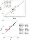 |
Fig. 6 Validity of analytical prescriptions. Top: dimensionless ratios Br/Bϕ versus |

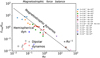 |
Fig. 7 Ratio of magnetic to kinetic energies as a function of the global shear parameter (dimensionless Rossby number) showing magnetostrophic scaling. |
6 Conclusions
Dynamo action in simplified models of radiative stellar layers can exhibit a rich diversity of magnetic field amplitudes and morphologies, including hemispherical dynamos. In particular, the dynamos found in the (sufficiently) strongly stratified regime are governed by magnetostrophic turbulence and achieve efficient AM transport, with measured Maxwell stresses in agreement with the diffusionless predictive scaling law of Spruit (2002). The existence of a dynamo similar to the Tayler–Spruit mechanism is observed in the computationally challenging regime of Rayleigh number up to Ra = 1010, confirming that the results reported in Petitdemange et al. (2023) pertain to even stronger stratification. Finally, intermediate scaling laws arising in the derivation of Spruit (2002) are carefully tested against our simulation results to assess the validity of the heuristic arguments in estimating magnetic stresses at saturation.
It should be pointed out, however, that our simulations provide a picture that is relatively far from the idealized situations considered in previous theoretical studies. The fundamental role of turbulent fluctuations or the presence of complex magnetic field geometry considerably complicates the interpretation within the framework of these theories. Although the results reported here reproduce many of the predictions of the Tayler–Spruit dynamo, we believe that our turbulent simulations describe a more general scenario, relevant to stellar interiors, but for which the canonical Tayler–Spruit or AMRI descriptions are only asymptotic limiting cases.
Full exploration of the parameter space is beyond the scope of the present study. The simulations presented here represent several millions of CPU hours, partly due to the necessity to integrate MHD equations over long times to rule out transient states, partly due to the computationally demanding flow regimes. Nevertheless, our numerical results already suggest that Tayler–Spruit dynamos pertain to a wider parameter regime as expected from the original theory: in particular, the analysis in Spruit (2002) relies on the hypothesis that N ≫ Ω, so that shellular approximation applies. The fact that our simulations with ratios Q of order unity or below still agree with Spruit’s original prescription is rather unexpected and shows the robustness of the Tayler–Spruit mechanism for rapid rotators. Whether this scaling law is modified or not at extreme values of the Reynolds, Rayleigh, or Ekman numbers, or for different ordering in the diffusivity ratios, remains to be discovered, however, and it would certainly be desirable to continue the numerical exploration of the parameter space as far as possible toward realistic parameter values.
Acknowledgements
The authors wish to thank Sacha Brun, Jim Fuller, Daniel Lecoanet, Frank Stefani and Miguel-Angel Aloy Toras for useful discussions. This work was granted access to the HPC resources of MesoPSL funded by the Region Île-de-France and the project Equip@Meso (reference ANR-10-EQPX-29-01) of the programme Investissements d’Avenir supervised by the Agence Nationale pour la Recherche. L.P. acknowledges financial support from “Programme National de Physique Stellaire” (PNPS) of CNRS/INSU, France. F.M. acknowledges financial support from the French program ‘T-ERC’ managed by Agence Nationale de la Recherche (Grant ANR-19-ERC7-0008-01). C.G. acknowledges financial support from the French program ‘JCJC’ managed by Agence Nationale de la Recherche (Grant ANR-19-CE30-0025-01).
References
- Aerts, C., Mathis, S., & Rogers, T. M. 2019, ARA&A, 57, 35 [Google Scholar]
- Aguirre, V. S., Stello, D., Stokholm, A., et al. 2020, ApJ, 889, L34 [Google Scholar]
- Aubert, J., Aurnou, J., & Wicht, J. 2008, Geophys. J. Int., 172, 945 [Google Scholar]
- Augustson, K. C., Brun, A. S., & Toomre, J. 2016, ApJ, 829, 92 [Google Scholar]
- Baglin, A., Auvergne, M., Barge, P., et al. 2009, in Transiting Planets, 253, eds. F. Pont, D. Sasselov, & M. J. Holman, 71 [NASA ADS] [Google Scholar]
- Borucki, W. J., Koch, D., Basri, G., et al. 2010, Science, 327, 977 [Google Scholar]
- Bugnet, L. 2020, PhD thesis, Université de Paris, France [Google Scholar]
- Cantiello, M., Mankovich, C., Bildsten, L., Christensen-Dalsgaard, J., & Paxton, B. 2014, ApJ, 788, 93 [Google Scholar]
- Ceillier, T., Eggenberger, P., García, R. A., & Mathis, S. 2013, A&A, 555, A54 [NASA ADS] [CrossRef] [EDP Sciences] [Google Scholar]
- Christophe, S., Ballot, J., Ouazzani, R. M., Antoci, V., & Salmon, S. J. A. J. 2018, A&A, 618, A47 [NASA ADS] [CrossRef] [EDP Sciences] [Google Scholar]
- Daniel, F., Petitdemange, L., & Gissinger, C. 2023, Phys. Rev. Fluids, 8, 123701 [NASA ADS] [CrossRef] [Google Scholar]
- Dormy, E. 2016, J. Fluid Mech., 789, 500 [NASA ADS] [CrossRef] [Google Scholar]
- Dormy, E., Cardin, P., & Jault, D. 1998, Earth Planet. Sci. Lett., 160, 15 [CrossRef] [Google Scholar]
- Dormy, E., Oruba, L., & Petitdemange, L. 2018, Fluid Dyn. Res., 50, 011415 [NASA ADS] [CrossRef] [Google Scholar]
- Eggenberger, P., Maeder, A., & Meynet, G. 2005, A&A, 440, L5 [Google Scholar]
- Eggenberger, P., Deheuvels, S., Miglio, A., et al. 2019, A&A, 621, A66 [NASA ADS] [CrossRef] [EDP Sciences] [Google Scholar]
- Eggenberger, P., Moyano, F. D., & den Hartogh, J. W. 2022, A&A, 664, A16 [NASA ADS] [CrossRef] [EDP Sciences] [Google Scholar]
- Fuller, J., Piro, A. L., & Jermyn, A. S. 2019, MNRAS, 485, 3661 [NASA ADS] [Google Scholar]
- Griffiths, A., Eggenberger, P., Meynet, G., Moyano, F., & Aloy, M.-Á. 2022, A&A, 665, A147 [NASA ADS] [CrossRef] [EDP Sciences] [Google Scholar]
- Guervilly, C., & Cardin, P. 2010, Geophys. Astrophys. Fluid Dyn., 104, 221 [NASA ADS] [CrossRef] [Google Scholar]
- Guseva, A., Hollerbach, R., Willis, A. P., & Avila, M. 2017, Phys. Rev. Lett., 119, 164501 [NASA ADS] [CrossRef] [Google Scholar]
- Ji, S., Fuller, J., & Lecoanet, D. 2023, MNRAS, 521, 5372 [NASA ADS] [CrossRef] [Google Scholar]
- Kirillov, O. N., Stefani, F., & Fukumoto, Y. 2014, J. Fluid Mech., 760, 591 [NASA ADS] [CrossRef] [Google Scholar]
- Maeder, A., & Meynet, G. 2000, ARA&A, 38, 143 [Google Scholar]
- Marcotte, F., Dormy, E., & Soward, A. 2016, J. Flurid Mech., 803, 395 [NASA ADS] [CrossRef] [Google Scholar]
- Mathis, S., Bugnet, L., Prat, V., et al. 2021, A&A, 647, A122 [EDP Sciences] [Google Scholar]
- Moffatt, H. K. 1978, Magnetic Field Generation in Electrically Conducting Fluids (Cambridge: Cambridge University Press) [Google Scholar]
- Petitdemange, L., Marcotte, F., & Gissinger, C. 2023, Science, 379, 300 [NASA ADS] [CrossRef] [Google Scholar]
- Philidet, J., Gissinger, C., Lignières, F., & Petitdemange, L. 2019, Gerophys. Astrophys. Fluid Dyn., 0, 1 [Google Scholar]
- Prat, V., Mathis, S., Neiner, C., et al. 2020, A&A, 636, A100 [NASA ADS] [CrossRef] [EDP Sciences] [Google Scholar]
- Proudman, I. 1956, J. Fluid Mech., 1, 505 [NASA ADS] [CrossRef] [Google Scholar]
- Rauer, H., Catala, C., Aerts, C., et al. 2014, Exp. Astron., 38, 249 [Google Scholar]
- Raynaud, R., Guilet, J., Janka, H.-T., & Gastine, T. 2020, Sci. Adv., 6, eaay2732 [NASA ADS] [CrossRef] [Google Scholar]
- Richardson, L., F. 1920, Proc. R. Soc. Lond., A97, 354 [NASA ADS] [Google Scholar]
- Rüdiger, G., Gellert, M., Hollerbach, R., Schultz, M., & Stefani, F. 2018, Physics Reports, 741, 1 [CrossRef] [Google Scholar]
- Salmon, S. J., Moyano, F. D., Eggenberger, P., Haemmerlé, L., & Buldgen, G. 2022, A&A, 664, L1 [NASA ADS] [CrossRef] [EDP Sciences] [Google Scholar]
- Schaeffer, N. 2013, Geochem. Geophys. Geosyst., 14, 751 [NASA ADS] [CrossRef] [Google Scholar]
- Schaeffer, N., Jault, D., Nataf, H.-C., & Fournier, A. 2017, Geophys. J. Int., 211, 1 [NASA ADS] [CrossRef] [Google Scholar]
- Seshasayanan, K., & Gallet, B. 2019, J. Fluid Mech., 864, 971 [NASA ADS] [CrossRef] [Google Scholar]
- Spruit, H. C. 2002, A&A, 381, 923 [CrossRef] [EDP Sciences] [Google Scholar]
- Stewartson, K. 1966, J. Fluid Mech., 26, 131 [NASA ADS] [CrossRef] [Google Scholar]
- Tayler, R. J. 1973, MNRAS, 161, 365 [CrossRef] [Google Scholar]
- Van Beeck, J., Prat, V., Van Reeth, T., et al. 2020, A&A, 638, A149 [NASA ADS] [CrossRef] [EDP Sciences] [Google Scholar]
- Van Reeth, T., Mombarg, J. S. G., Mathis, S., et al. 2018, A&A, 618, A24 [NASA ADS] [EDP Sciences] [Google Scholar]
- Wade, G. A., Neiner, C., Alecian, E., et al. 2016, MNRAS, 456, 2 [Google Scholar]
- Wheeler, J. C., Kagan, D., & Chatzopoulos, E. 2015, ApJ, 799, 85 [NASA ADS] [CrossRef] [Google Scholar]
- Zahn, J.-P. 1974, Symp. Int. Astron. Union, 59, 185 [NASA ADS] [CrossRef] [Google Scholar]
- Zahn, J.-P. 1992, A&A, 265, 115 [NASA ADS] [Google Scholar]
- Zahn, J.-P., Brun, A. S., & Mathis, S. 2007, A&A, 474, 145 [NASA ADS] [CrossRef] [EDP Sciences] [Google Scholar]
All Figures
|
Fig. 1 Stratification influence on the onset of shear instability in a spherical shell. Top: evolution of the critical Reynolds number Rec (or equivalently the Rossby number Roc) as a function of stratification intensity (quantified by the Rayleigh number Ra). When Re > Rec (red upward triangles), nonaxisymmetric modes are maintained in time. Conversely, when Re < Rec (dark downward triangles), the kinetic energies of nonaxisymmetric modes exponentially decay with time. The insets highlight the pattern of unstable modes close to the threshold via color maps of the radial velocity in the equatorial plane. Simulations parameters: E = 10−5, Pr = 0.1. Bottom: critical Reynolds number Rec for the onset of hydrodynamic instability with increasing stratification, for various thermal and rotation parameters. |
| In the text | |
|
Fig. 2 Time-averaged magnetic energy for dynamo simulations performed with different parameters and initial conditions for the magnetic field. The stars correspond to models in which the axisymmetric toroidal magnetic component exceeds 80% of the total magnetic energy (toroidal dynamos). The fixed simulation parameters are E = 10−5, Pr = 0.1, Pm = 1. |
| In the text | |
|
Fig. 3 Meridional sections of the axisymmetric components of azimuthal magnetic Bϕ, radial magnetic field Br, and angular velocity Ω⋆ (normalized by ΔΩ). Top: weakly stratified dipolar dynamo at E = 10−5, Ra = 107, Re = 5000, Pr = 0.1, Pm = 1. Middle: hemispherical dynamo at E = 10−5, Ra = 108, Re = 12000, Pr = 0.1, Pm = 1. Bottom: strong toroidal (Tayler–Spruit) dynamo at E = 10−5, Ra = 1010, Re = 3.104, Pr = 0.1, Pm = 1. |
| In the text | |
|
Fig. 4 Meridional sections of axisymmetric latitudinal and radial components of the velocity field (left) and magnetic field (right). Parameters: Re = 2.75 × 10⁴ and Ra = 109 (uppel panel; Q = 0.15); Re = 3.104 and Ra = 1010 (lower panel; Q = 1.5). The other control parameters are fixed as in Fig. 3. |
| In the text | |
|
Fig. 5 Distribution of axisymmetric and nonaxisymmetric magnetic components. Top: radial profile of the magnetic Rossby number Rb and the axisymmetric azimuthal field |
| In the text | |
|
Fig. 6 Validity of analytical prescriptions. Top: dimensionless ratios Br/Bϕ versus |
| In the text | |
|
Fig. 7 Ratio of magnetic to kinetic energies as a function of the global shear parameter (dimensionless Rossby number) showing magnetostrophic scaling. |
| In the text | |
Current usage metrics show cumulative count of Article Views (full-text article views including HTML views, PDF and ePub downloads, according to the available data) and Abstracts Views on Vision4Press platform.
Data correspond to usage on the plateform after 2015. The current usage metrics is available 48-96 hours after online publication and is updated daily on week days.
Initial download of the metrics may take a while.