| Issue |
A&A
Volume 695, March 2025
|
|
|---|---|---|
| Article Number | A183 | |
| Number of page(s) | 17 | |
| Section | Astrophysical processes | |
| DOI | https://doi.org/10.1051/0004-6361/202451337 | |
| Published online | 18 March 2025 | |
Tayler-Spruit dynamo in stably stratified rotating fluids: Application to proto-magnetars
1
Université Paris-Saclay, Université Paris Cité, CEA, CNRS, AIM, 91191 Gif-sur-Yvette, France
2
Observatoire de Genève, Université de Genève, 51 Ch. Pegasi, 1290 Versoix, Switzerland
3
Université Paris Cité, Université Paris-Saclay, CNRS, CEA, AIM, 91191 Gif-sur-Yvette, France
4
Max Planck Institute for Gravitational Physics (Albert Einstein Institute), D-14476 Potsdam, Germany
⋆ Corresponding author; This email address is being protected from spambots. You need JavaScript enabled to view it.
Received:
1
July
2024
Accepted:
13
February
2025
Abstract
The formation of highly magnetized young neutron stars, called magnetars, is still a strongly debated topic. One promising scenario invokes the amplification of the magnetic field by the Tayler-Spruit dynamo in a proto-neutron star (PNS) that is spun up by fall-back. Our previous numerical study supports this scenario by demonstrating that this dynamo can generate magnetar-like magnetic fields in stably stratified Boussinesq models of a PNS interior. To further investigate the Tayler-Spruit dynamo, we performed 3D magnetohydrodynamic (MHD) numerical simulations with the MagIC code, varying the ratio between the Brunt-Väisälä frequency and the rotation rate. We first demonstrated that a self-sustained dynamo process can be maintained for a Brunt-Väisälä frequency about four times higher than the angular rotation frequency. The generated magnetic fields and angular momentum transport follow the scaling laws derived in prior analytical investigations, confirming our earlier results. We also report, for the first time, the existence of an intermittent Tayler-Spruit dynamo. For a typical PNS Brunt-Väisälä frequency of 1 kHz, the axisymmetric toroidal and dipolar magnetic fields range between 1.2 × 10¹⁵–2 × 10¹⁶ G and 1.4 × 10¹³–3 × 10¹⁵ G, for rotation periods of 1 − 10 ms. Moreover, the total magnetic field remains ≳1014 G for periods of ≲60 ms. Thus, our results suggest that our scenario is promising to form classical fast-rotating magnetars and magnetars with weaker magnetic dipoles for slower rotations. We offer a calibration of the analytical scaling laws based on our simulations, with a dimensionless normalisation factor of the order of 10−2. As the Tayler-Spruit dynamo is often invoked for the angular momentum transport in stellar radiative zones, our results are of particular significance to asteroseismology as well.
Key words: dynamo / magnetohydrodynamics (MHD) / methods: numerical / stars: magnetars / stars: magnetic field / supernovae: general
© The Authors 2025
 Open Access article, published by EDP Sciences, under the terms of the Creative Commons Attribution License (https://creativecommons.org/licenses/by/4.0), which permits unrestricted use, distribution, and reproduction in any medium, provided the original work is properly cited.
This article is published in open access under the Subscribe to Open model. This email address is being protected from spambots. You need JavaScript enabled to view it. to support open access publication.
1. Introduction
Soft gamma repeaters and anomalous X-ray pulsars are two classes of neutron stars (NSs) that exhibit a wide variety of high-energy emissions, from short chaotic bursts during outbursts phases (e.g. Gotz et al. 2006; Younes et al. 2017; Coti Zelati et al. 2018, 2021) to giant flares (Evans et al. 1980; Hurley et al. 1999, 2005; Svinkin et al. 2021), which are the brightest events observed in the Milky Way. These neutron stars are called magnetars because their emissions have been shown to be powered by the dissipation of their ultra-strong magnetic fields (Kouveliotou et al. 1994). Indeed, these emissions show that they rotate with periods of 2 − 12 s and have stronger rotation braking than typical NSs (e.g. Rea et al. 2012; Olausen & Kaspi 2014). If the spin-down is due to the extraction of rotational energy by a magnetic dipole, we can infer that most magnetars exhibit a surface magnetic dipole of 1014–1015 G, namely, the strongest known in the Universe. Three magnetars, however, display weaker magnetic dipoles of 6 × 10¹²–4 × 10¹³ G (Rea et al. 2010, 2012, 2013, 2014), but absorption lines detected in the X-ray spectra of two of these magnetars suggest the presence of stronger non-dipolar magnetic fields of 2 × 10¹⁴–2 × 10¹⁵ G (Tiengo et al. 2013; Rodríguez Castillo et al. 2016). These ‘low-field’ magnetars therefore demonstrate that an ultra-strong surface magnetic dipole is not necessary for a NS to produce magnetar-like emission.
Magnetars are also suspected to be the central engine of extreme events. In combination with a millisecond rotation period, magnetars in their proto-neutron star (PNS) stage may power magnetorotational supernova (SN) explosions which are more energetic than typical neutrino-driven SNe (e.g. Burrows et al. 2007; Dessart et al. 2008; Takiwaki et al. 2009; Kuroda et al. 2020; Bugli et al. 2020, 2021, 2023; Obergaulinger & Aloy 2020, 2021, 2022). The formation of a millisecond magnetar is a popular scenario to explain super-luminous SNe (Woosley 2010; Kasen & Bildsten 2010; Dessart et al. 2012; Inserra et al. 2013; Nicholl et al. 2013) and hypernovae, the latter of which are associated to long gamma-ray bursts (GRBs ; Duncan & Thompson 1992; Zhang & Mészáros 2001; Woosley & Bloom 2006; Drout et al. 2011; Nomoto et al. 2011; Gompertz & Fruchter 2017; Metzger et al. 2011, 2018). In the case of binary NS mergers, the NS remnant may be a magnetar whose magnetic fields power the plateau phase observed in short GRBs afterglows (e.g. Lü & Zhang 2014; Gompertz et al. 2014; Kiuchi et al. 2024).
Recently, the observation of the fast radio burst FRB 200428 was associated to X-ray bursts of the magnetar SGR 1935+2154 (Bochenek et al. 2020; CHIME/FRB Collaboration 2020; Mereghetti et al. 2020; Zhu et al. 2023; Tsuzuki et al. 2024), which supports magnetar-powered emission scenarios to explain at least a fraction of FRBs. To better understand these phenomena, it is thus essential to investigate the question of magnetar formation and especially the origin of their ultra-strong magnetic fields. The association of a few magnetars with SN remnants suggests that they are born during core-collapse SNe (Vink & Kuiper 2006; Martin et al. 2014; Zhou et al. 2019). The magnetic fields could be amplified during the core-collapse due to the magnetic flux conservation (Ferrario & Wickramasinghe 2006; Hu & Lou 2009; Schneider et al. 2019; Shenar et al. 2023). However, the magnetic field of the iron core of the progenitor star is not constrained by observations and it is uncertain whether this scenario can explain the whole magnetar population (Makarenko et al. 2021). A second type of scenario invokes a dynamo action in the newly formed PNS to generate strong large-scale magnetic fields. Three mechanisms have been studied: the convective dynamo (Thompson & Duncan 1993; Raynaud et al. 2020, 2022; Masada et al. 2022; White et al. 2022), the magnetorotational instability (MRI)-driven dynamo (Obergaulinger et al. 2009; Mösta et al. 2014; Rembiasz et al. 2017; Reboul-Salze et al. 2021, 2022; Guilet et al. 2022), and the Tayler-Spruit dynamo (Barrère et al. 2022, 2023).
The two former dynamos have been shown to form magnetar-like magnetic fields in the case of fast rotation. In the framework of the millisecond magnetar model, these mechanisms are therefore promising to explain the formation of the central engine extreme explosions. Nevertheless, two uncertainties remain. First, SN remnants associated with magnetars show typical explosion energy of ∼1051 erg. This implies that most magnetars were born in standard core-collapse supernovae (CCSNe), which requires slower rotation, with periods of at least 5 ms (Vink & Kuiper 2006). Second, the rotation is assumed to stem from a fast-rotating progenitor core. It is unclear whether there is a large enough fraction of these progenitors to explain the entire magnetar population, which constitutes ∼10% of young NSs.
To address these points, in Barrère et al. (2022), we developed a new formation scenario in which the PNS rotation is determined by the fall-back, namely, the matter that is initially ejected by the SN explosion before eventually falling back onto the PNS. In particular, 3D CCSNe numerical simulations have shown that the fall-back accretion can significantly spin up the PNS surface (Chan et al. 2020; Stockinger et al. 2020; Janka et al. 2022). We argued that the differential rotation caused by this spin-up triggers the development of the Tayler-Spruit dynamo. This dynamo mechanism is driven by the combination of the differential rotation and the Tayler instability, which is an instability triggered by perturbations of a purely toroidal magnetic field (Tayler 1973; Goossens & Tayler 1980; Ma & Fuller 2019; Skoutnev & Beloborodov 2024a,b). Studies in stellar evolution (e.g. Eggenberger et al. 2005; Cantiello et al. 2014; Eggenberger et al. 2019a,b; den Hartogh et al. 2020; Griffiths et al. 2022) often rely on this mechanism to explain the strong angular momentum transport (AMT) inferred via asteroseismology in sub-giant and red giant stars (e.g. Mosser et al. 2012; Deheuvels et al. 2014, 2015; Gehan et al. 2018). Like our model in Barrère et al. (2022), these works use analytical prescriptions to model the AMT produced by the large-scale magnetic fields in stellar radiative zones. Two distinct analytical models of the Tayler-Spruit dynamo have been used: the original model of Spruit (2002) and the revised one of Fuller et al. (2019), which tackles previous criticisms of the original model. The prescriptions, however, cannot take into account the strong non-linearity behind the dynamo mechanism, which calls for numerical investigations of its 3D complex dynamics to better characterize its effects in both astrophysical contexts.
Petitdemange et al. (2023, 2024), Daniel et al. (2023) performed 3D direct numerical simulations of dynamo action in a stably stratified Couette flow in the context of stellar radiative layers, in which the inner core rotates faster than the outer layer. They argued that the dynamo was driven by the Tayler instability and found scaling laws in agreement with the prescriptions of Spruit (2002). In our numerical study Barrère et al. (2023), the set-up is different, with an outer sphere rotating faster than the core, which is relevant to our magnetar formation scenario. We demonstrated the existence of more complex dynamics with two Tayler-Spruit dynamo branches, which have distinct magnetic field strengths and geometries: the weaker branch shows a hemispherical field, while the strongest one displays a dipolar symmetry. Furthermore, the former follows the analytical scaling of Spruit (2002), while the latter is in agreement with the predictions of Fuller et al. (2019). Lastly, the dipolar dynamo could reach axisymmetric toroidal and dipole magnetic fields up to ∼2 × 10¹⁵ G and ∼3 × 10¹⁴ G, respectively. Although such intensities seem relevant to form magnetars, these models considered only a fixed ratio of the Brunt-Väisälä to the surface angular frequency N/Ωo = 0.1, whereas it is expected to cover the range of N/Ωo ∈ [0.1, 10] in real PNSs (N ∼ 1 × 10³ s−1 and Ωo ∼ 102–104 rad s−1).
Therefore, this article is aimed at investigating the impact of the stratification N/Ωo on the dipolar Tayler-Spruit dynamo discovered in Barrère et al. (2023). The study of the hemispherical dynamo will lead to another paper that will be more focused on the complex physics behind the Tayler-Spruit dynamos. In the following, Sect. 2 describes the governing equations and the numerical set-up of our simulations. We present the results in Sect. 3, which will be applied to the question of magnetar formation in Sect. 4. Finally, we discuss the results and conclude in Sect. 5 and Sect. 6, respectively.
2. Numerical set-up
2.1. Governing equations
As in Barrère et al. (2023), we used an idealised model of the PNS meant to approximately represent the conditions prevailing at times later than 5-10 s after core bounce, when the fall-back accretion is taking place. The PNS has a mass of M = 1.4 M⊙ and a radius of ro = 12 km, which corresponds to the typical PNS radius after the contraction phase (e.g. Hüdepohl 2014; Pascal et al. 2022). Its interior consists of a stably stratified and electrically conducting fluid evolving between two concentric spheres, which rotate at constant rotation rates. For the sake of simplicity and computational efficiency, we adopted the Boussinesq approximation (see Sect. 5.4 for a discussion), which assumes a constant background density profile with ρ = 3.8 × 10¹⁴ g cm−3, but takes into account the buoyancy force due to entropy and electron fraction perturbations. In the reference frame rotating with the surface at the angular velocity Ωo = Ωoez, the Boussinesq magnetohydrodynamic (MHD) equations are expressed as:
 (1)
(1)
 (2)
(2)
 (3)
(3)
 (4)
(4)
 (5)
(5)
where B is the magnetic field, v is the velocity field, p′ is the non-hydrostatic pressure, ρ is the mean density of the PNS, and α ≡ ρ−1(∂Tρ)p is the thermal expansion coefficient. Also, ez and er are the unit vectors of the axial and the spherical radial directions, respectively. Θ is the buoyancy variable defined by
 (6)
(6)
where g = gor/ro is the gravitation field consistent with a constant density profile. ρ′ is the density perturbation due to the combined effect of the electron fraction and entropy perturbations and
 (7)
(7)
is the Brunt-Väisälä frequency with the electron fraction, Ye, and the entropy, S, respectively.
In the above equations, we assume that the magnetic diffusivity, η, the kinematic viscosity, ν, and the “thermal” diffusivity, κ are constant. We also assume that the thermal and lepton number diffusivities are equal, which allows us to describe the buoyancy associated with both entropy and lepton number gradients with the use of a single buoyancy variable Θ (Guilet et al. 2015).
Apart from the magnetic diffusivity which relates to the electrical conductivity of electrons, the physical interpretation of the other transport coefficients can lead to different estimates, depending on whether or not neutrinos are considered to be the main source of diffusive processes (see Sect. 1.3 of the supplementary materials in Barrère et al. 2023).
The inner boundary condition is a sphere with a radius of radius ri = 3 km. This inner sphere does not exist in a PNS but enables us to control the fluid differential rotation. We leave an investigation of the influence of using a larger domain or a full sphere for future study. The forcing of the differential rotation, in the so-called spherical Taylor-Couette configuration, is controlled by no-slip boundary conditions with fixed rotation rate at each boundary. This is a crude proxy of the spin-up due to accretion and does not take into account the growth of the surface rotation rate at the beginning of the fall-back phase, nor the evolution of the fall-back accretion rate (see Sect. 5.3 for a discussion). Finally, we applied electrically insulating and fixed buoyancy variable boundary conditions on both spheres.
2.2. Numerical methods
We used the open source pseudo-spectral code MagIC1 (Wicht 2002; Gastine & Wicht 2012; Schaeffer 2013) to integrate Eqs. (1)–(5) into 3D spherical geometry. To satisfy the solenoidal conditions (1) and (5), the velocity and magnetic fields must be decomposed in poloidal and toroidal components (Mie representation),
 (8)
(8)
 (9)
(9)
where W and Z (b and aj) are the poloidal and toroidal potentials for the velocity (magnetic) field. The whole system of equations is then solved in spherical coordinates by expanding the scalar potentials in Chebyshev polynomials in the radial direction and spherical harmonic functions in the angular directions. The time-stepping scheme used is the implicit/explicit Runge-Kutta BPR353 (Boscarino et al. 2013). We refer to the MagIC online documentation2 for an exhaustive presentation of the numerical techniques.
2.3. Input parameters
The resistivity is controlled by the magnetic Prandtl number Pm ≡ ν/η. Although its realistic value in PNSs (Pm ∼ 1011, Barrère et al. 2023) cannot be reached by numerical simulations, we can remain in the Pm ≥ 1 regime by imposing Pm ∈ [1, 4].
The imposed stable stratification is characterized by the Brunt-Väisälä frequency N (Eq. (7)). In our parameter study, the ratio N/Ωo was varied between 0.1 and 10 and so, we were able to cover the PNS regime. In practice, this ratio is related to the Rayleigh number Ra ≡ −(N/Ω)2Pr/E2, which is negative in the regime of stable stratification.
We kept the other dimensionless control parameters fixed: the shell aspect ratio χ ≡ ri/ro = 0.25 and width d ≡ ro − ri, Ekman number E ≡ ν/(d2Ωo) = 10−5, thermal Prandtl numbers Pr ≡ ν/κ = 0.1, and the Rossby number Ro ≡ 1 − Ωi/Ωo = 0.75, which controls the imposed differential rotation. Finally, the resolution was set at (nr, nθ, nϕ) = (257, 256, 512) for all the runs.
The simulations were initialized either from a nearby saturated state or a strong toroidal axisymmetric field with a dipolar equatorial symmetry, namely, equatorially symmetric3 with l = 2, m = 0. We note that the saturated state of the dynamo does not depend on the initial magnetic field if it is above the threshold for dynamo action (see Appendix A). We define a turbulent resistive time  , where
  is the typical value of the average harmonic degree of the time-averaged magnetic energy spectrum. In the following, we will term a solution ‘transient’ when a steady state is sustained for a time interval
  , and ‘stable’ for
  .
.
We start with the run named ‘Ro0.75s’ from Barrère et al. (2023), where the stratification is N/Ωo = 0.1. The saturated state of this dynamo is used to initialise the next simulation with a stronger stratification. The whole set of simulations is initiated similarly using the nearby saturated state of a less stratified run. With this procedure, N/Ωo is increased gradually in order to study the evolution of the dynamo branch.
2.4. Output parameters
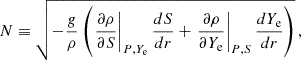
We first characterized our models by computing the time average of the kinetic and magnetic energy densities (after filtering out any initial transient). The latter is expressed in terms of the viscous Elsasser number Λν ≡ Λ/Pm = Brms2/(4πρνΩo) and used to compute different root-mean-square (RMS) estimates of the magnetic field. In addition to the total field, we distinguish the poloidal and toroidal fields based on the Mie representation (Sect. 2.2), while the dipole field refers to the l = 1 poloidal component.
3. Results
The following sections present the different results we obtain from the set of numerical simulations listed in Appendix C. We first describe the global dynamics of the dipolar Tayler-Spruit dynamo in the parameter space in Sect. 3.1. Then, we analyse the influence of stratification on the modes of Tayler instability and on the generated axisymmetric magnetic fields in their saturated state in Sects. 3.3 and 3.4, respectively. We also present the angular momentum transport by both Reynolds and Maxwell stresses due to the dynamo and compare the efficiencies of mixing and angular momentum transport in Sect. 3.5. Finally, we examine a new intermittent behaviour of the Tayler-Spruit dynamo at N/Ωo ≥ 2, which is observed for the first time (see Sect. 3.6).
3.1. Subcritical dynamo sustained at PNS-like stratifications
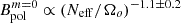
Figure 1 shows that a self-sustained Tayler-Spruit dynamo can be maintained up to N/Ωo = 1 for Pm = 1. For a stronger stratification, we have to increase Pm (i.e. decrease the resistivity) to maintain the dynamo. For Pm = 4, the stationary state was self-sustained up to N/Ωo = 4 and we obtained transient states up to N/Ωo = 10. The self-sustained dynamo is therefore present below the threshold for the fluid to be hydrodynamically stable at N/Ωo ∼ 1.5. This confirms the subcritical nature of the Tayler-Spruit dynamo, which was already observed in previous studies (Petitdemange et al. 2023; Barrère et al. 2023). We did not simulate fluids at greater Pm values for reasons of numerical costs. Given the trend with Pm observed in our simulations as well as theoretical expectations on the Tayler instability threshold, we would expect the Tayler-Spruit dynamo to exist at still higher values of N/Ω for the higher values of Pm relevant to a PNS.
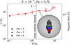 |
Fig. 1. Viscous Elsasser number (and RMS magnetic field) as a function of the ratio of the Brunt-Väisälä frequency to the rotation rate at the outer sphere. Filled and empty markers represent self-sustained and transient dynamos, respectively. The black dashed vertical line and arrow indicate the zone in which the fluid is hydrodynamically unstable. The inset represents a 3D plot of the radial velocity (violet and green isosurfaces are the positive and negative values, respectively) and the radial magnetic field (red and blue isosurfaces are the positive and negative values, respectively) in a run at Pm = 2 and N/Ωo = 2. The grey arrow points to the run location in the diagram. |
3.2. Impact on the differential rotation
The meridional slices of the angular rotation frequency Ω illustrate the impact of stable stratification on the rotation profile: we see that the shear concentrates closer to the inner sphere and increases with N/Ωo. At the same time, the rotation profile smoothly transits from a quasi-cylindrical to a spherical geometry, which is an effect already observed in stably stratified flows. Analytical and numerical studies of these flows (e.g. Barcilon & Pedlosky 1967a,b,c; Gaurat et al. 2015; Philidet et al. 2020) indicate that this transition is controlled by the dimensionless parameter Q ≡ Pr(N/Ωo)2, which varies between 10−3 and 10 in our set of runs. The change in the flow geometry is therefore explained by a transition from a case where neither the rotation nor the buoyancy dominate (E2/3 < Q < 1) to a buoyancy-dominated flow (Q ≫ 1).
3.3. Impact on the Tayler modes
As seen in Fig. 3, the unstable magnetic modes are located close to the poles where the latitudinal gradient of Bϕ is positive, which is a first indication supporting the presence of Tayler modes. To confirm this assumption, we can use the geometrical criterion of Goossens & Tayler (1980) for the stability of m = 1-modes,
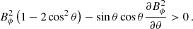 (10)
(10)
The stability regions displayed by the hatched zones in Fig. 3 match very well regions where the unstable modes are absent. This confirms that the Tayler instability is clearly identifiable, no matter the values of N/Ωo.
Moreover, the impact of stratification on the mode structure is striking. The stable stratification tends to stabilise displacements in the radial direction, as we can see looking at the non-axisymmetric radial velocity vrm ≠ 0 field in Fig. 2. As a consequence, the radial length scale of the instability strongly decreases for increasing values of N/Ωo. This feature is not surprising because Spruit (1999) already constrained the mode maximum radial length scale
 |
Fig. 2. Meridional slices of the angular frequency and the non-axisymmetric radial velocity (left and right slices respectively) for different values of N/Ωo at t = 5650 Po, t = 7792 Po, t = 2967 Po, and t = 287 Po, respectively, with Po ≡ 2π/Ωo. Ω and vrm ≠ 0 are scaled by Ωo and roΩo, respectively. |
 |
Fig. 3. Meridional slices of the axisymmetric azimuthal and the s = r sin θ-component of the magnetic field (respective left and right slices) for increasing values of N/Ωo at t = 5650 Po, t = 7792 Po, t = 2967 Po, and t = 287 Po, respectively, with Po ≡ 2π/Ωo. The magnetic field is scaled by |

 (11)
(11)
where  is the Alfvén frequency. We note that a lower limit due to resistivity is also predicted
 (12)
(12)
The length scales measured in our models are compared to these constraints in Fig. 4. Since thermal diffusion can mitigate the effect of stratification, we can also define an effective Brunt-Väisälä frequency,
 (13)
(13)
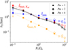 |
Fig. 4. Length scale of the Tayler instability mode measured in the simulations (black stars) as a function of N/Ωo. The theoretical lower (lmin in blue) and upper boundaries of the length scale are also plotted using the classical (lmax, N in orange) and the effective (lmax, Neff in red) Brunt-Väisälä frequencies. Filled and empty markers represent self-sustained and transient dynamos, respectively. |
and so,
 (14)
(14)
thereby taking this effect into account (Spruit 2002). The Tayler modes in our simulations have length scales ranging from ro/4 = 3 km at N/Ωo = 0.1 to ro/80 = 0.15 km at N/Ωo = 10. This implies that resolving the Tayler-Spruit dynamo requires higher and higher resolutions as the stratification increases. The measured lTI follows very well the upper limit lmax, Neff (red points in Fig. 4), but is around one order of magnitude larger than lmax, N. This demonstrates the importance of including the mitigation of the stratification by diffusion. The minimum length scale lmin (Eq. (12)) is almost equal to lTI from N/Ωo = 0.5 to N/Ω = 4, which indicates that we are close to the instability threshold. For N/Ωo ≥ 6, however, lmin ∼ 2lmax, Neff ∼ 2 − 3lTI. The fluid is therefore stable, which is consistent with the transient state we find in our simulations. Thus, the analytical limits for the Tayler modes to develop are validated by our numerical simulations and suggest that the Tayler-Spruit dynamo could be maintained for N/Ωo ∈ [6, 10] with Pm ≳ 16 − 36.
In addition to the decrease of the radial length scale lTI, the Tayler instability modes are strongly affected by high values of N/Ωo. The time and volume averaged spectra of the magnetic energy in Fig. 5 show that the energy of the large-scale (l = 1 − 10) non-axisymmetric modes (solid lines) drop by two orders of magnitude between N/Ω = 0.25 and at N/Ω = 2 compared to the energy of the dominant axisymmetric toroidal component (blue dotted line). This difference is represented more quantitatively by comparing the total non-axisymmetric magnetic field  to
to  in Fig. 6. The ratio drops from ∼1 to ∼2 × 10⁻³ and follows a power law
 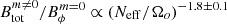 . Fuller et al. (2019) analytically derived that the ratio between the magnetic field generated by the Tayler instability (noted
  ) and
) and  scales as ωA/Ωo. Since ωA ∝ (Neff/Ωo)−1/3 (Fuller et al. 2019, and our Sect. 3.4), our simulations therefore do not match this analytical prediction. Fuller et al. (2019) derived the ratio by equating the Tayler instability growth rate and a turbulent damping rate ωA2/Ωo ∼ δvA/r, where
 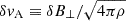 . As the growth rate of the Tayler instability is robust (Zahn et al. 2007; Ma & Fuller 2019) and well verified in numerical simulations (Ji et al. 2023), our study then questions the estimate of the turbulent damping rate.
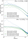 |
Fig. 5. Time- and volume-averaged spectra of the magnetic energy for the parameters Pm = 1, N/Ωo = 0.25 (top), and Pm = 2, N/Ωo = 2 (bottom). The magnetic energy is normalized by the energy of the dominant (ℓ = 2, m = 0)-mode of the toroidal component. |
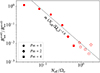 |
Fig. 6. Ratio of the RMS non-axisymmetric magnetic field to the RMS axisymmetric toroidal magnetic field. The dotted line shows the best fit for a power law of Neff/Ωo. The filled and empty markers represent self-sustained and transient dynamos, respectively. |
3.4. Magnetic field saturation
As in Barrère et al. (2023), we confronted the saturated large-scale magnetic fields in our simulations to the analytical predictions. To this end, we first measure the impact of the stratification on the local shear rate, q, which influences the magnetic field saturation. Indeed, the rotation profiles of Fig. 2 show that the shear concentrates closer to the inner sphere and increases with N/Ωo. The quantification of this effect is described in Appendix B. These larger values of q explain the increase of the magnetic energy with N/Ωo observed in Fig. 1.
To study the relation of the magnetic field components with Neff/Ωo while taking into account the variation of q, we use the analytical prescriptions derived by Fuller et al. (2019):
 (15)
(15)
 (16)
(16)
The exponents of q are all the more robust as they are confirmed by numerical simulations (Barrère et al. 2023). We define dimensionless magnetic field components compensated for the effect of the shear in the following way:
 (17)
(17)
 (18)
(18)
These compensated dimensionless components are plotted in Fig. 7 as a function of Neff/Ωo. The theoretical scaling laws (dotted black lines) qualitatively match our data. Since the point at Neff/Ωo = 3 × 10⁻² diverges from the scalings due to the weaker effect of stable stratification, we exclude it while calculating the best fits. We obtain the following power-laws  ,
,  , and Bdip ∝ (Neff/Ωo)−1.5 ± 0.1. While
  and
and  follow power-laws slightly less steep than predicted in Eqs. (15) and (16), Bdip is in good agreement with Eq. (16).
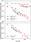 |
Fig. 7. RMS toroidal and poloidal axisymmetric magnetic fields (top), and RMS magnetic dipole (bottom) compensated with the measured shear rate as a function of the ratio between the effective Brunt-Väisälä frequency to the rotation rate at the outer sphere Neff/Ωo. The magnetic field is rendered dimensionless and compensated for the effect of the shear using Eqs. (17) and (18). Dotted lines show the best fits of the data with Fuller’s theoretical scaling laws (Eqs. (15) and (16)) within a multiplying factor. Filled and empty markers represent self-sustained and transient dynamos, respectively. |
This agreement with the theory is also found for the ratio  (Spruit 2002; Fuller et al. 2019), as seen in Fig. 8. Our data is fitted by the power law
 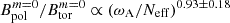 , which is very close to the prediction. On the other hand, the ratio of the magnetic dipole to the axisymmetric toroidal field follows a somewhat steeper scaling law
  .
.
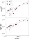 |
Fig. 8. Ratio between the RMS axisymmetric poloidal (top) and the RMS dipolar (bottom) magnetic fields to the axisymmetric toroidal magnetic field. Dotted lines show the best fits to the data with Fuller’s theoretical scaling law Br/Bϕ ∼ ωA/Neff, within a multiplying factor. Filled and empty markers represent self-sustained and transient dynamos, respectively. |
3.5. Angular momentum transport and mixing
The angular momentum transport due to the large-scale magnetic field and turbulence in our simulations is also consistent with the theory of Fuller et al. (2019), as shown in Fig. 9. For the Maxwell torque, TM, we find BsBϕ ∝ (Neff/Ωo)−1.8 ± 0.1 and  , depending on whether we take the non-axisymmetric components into account in TM. We note that the torque is more and more dominated by the axisymmetric magnetic fields as Neff/Ωo increases. This dominance was assumed by Fuller et al. (2019) and can be expected given the results of Sect. 3.3. The Reynolds torque values are more dispersed as a function of the stratification, but fit the power laws
  and
and  . Despite some scattering at high values of Neff/Ωo in the points corresponding to transient dynamos, our data therefore follow the analytical predictions TM ∝ (Neff/Ωo)−2 and TR ∝ (Neff/Ωo)−10/3 (dotted lines in Fig. 9) quite well. Moreover, we find TM ∼ 102–103 TR, so the magnetic field is much more efficient than turbulence at transporting angular momentum.
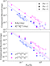 |
Fig. 9. RMS Maxwell (top) and Reynolds (bottom) torques compensated with the measured shear rate as a function of the ratio between the effective Brunt-Väisälä frequency to the rotation rate at the outer sphere. Dotted lines show the best fits obtained with Fuller’s theoretical scaling laws. Filled and empty markers represent self-sustained and transient dynamos, respectively. |
The mixing processes are also a crucial question in astrophysics, especially for stars. The Tayler-Spruit dynamo is expected to produce a very limited mixing efficiency compared to the angular momentum transport (Spruit 2002; Fuller et al. 2019). To measure this effect in our simulations, we define the effective angular momentum transport diffusivity νAM ≡ TM/(ρqΩo) and roughly approximate the effective mixing diffusivity as νmix ≡ q−5/3vm ≠ 0lTI, with the RMS turbulent velocity  calculated from the mean non-axisymmetric energy
  . We divided by the power law q5/3 in the expression of νmix to take into account the variation of q (as in Figs. 7 and 9).
The ratio νmix/νAM plotted in Fig. 10 demonstrates that our data are in fair agreement with the scaling νmix/νAM ∝ Neff/Ωo−5/3 of Fuller et al. (2019). The power law νmix/νAM ∝ Neff/Ωo−1.2 ± 0.2 best fits our data, which is mildly less steep than predicted. Moreover, our simulations also confirm that νmix/νAM ∼ 10−6–10−3 ≪ 1 for Tayler-Spruit dynamo. The use of passive scalars evolving in the velocity field in our simulations could help measure νmix more precisely, even though the approximation we used is satisfactory as a first analysis.
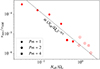 |
Fig. 10. Ratio of the effective mixing diffusivity, νmix, to the effective angular momentum diffusivity, νAM, as a function of Neff/Ωo. Filled and empty markers represent self-sustained and transient dynamos, respectively. |
Table 1 sums up the comparisons we have done between our data and the different scalings derived by Fuller et al. (2019). Our results thus consolidate the validity of Fuller et al. (2019)’s formalism for the saturation of large-scale magnetic fields and angular momentum transport. Besides, our simulations are not compatible with the analytical prescriptions of Spruit (2002), which are expressed as
 (19)
(19)
 (20)
(20)
 (21)
(21)
Theoretical and measured scaling laws of the different quantities discussed in Sects. 3.4 and 3.5, and the dimensionless normalisation factor α defined by Fuller et al. (2019) and Eq. (22).
While our simulations support the scaling law of Fuller et al. (2019), we can also constrain the dimensionless normalisation factor (noted α in Fuller et al. 2019), that parametrises the saturated strength of the axisymmetric toroidal magnetic field:
 (22)
(22)
We inferred the value of α by fitting our data by the theoretical scaling law. The measurements are listed in the last column of Table 1 and we find a mean value of α ∼ 10−2. This value is small compared to those inferred by adjusting α in 1D stellar evolution models to the asteroseismic observations of sub- and red giants, which is ∼0.25 − 1 (Fuller et al. 2019; Fuller & Lu 2022; Eggenberger et al. 2019b). Either way, our numerical simulations provide a more physically motivated value of α that could be implemented in 1D stellar evolution codes, including the Tayler-Spruit dynamo to transport angular momentum.
3.6. Intermittency
When N/Ωo ≥ 2, we find that the Tayler-Spruit dynamo displays an intermittent behaviour. This is clearly visible in the time series of Fig. 11, where the non-axisymmetric magnetic energy drops and increases cyclically by two orders of magnitude. This corresponds to the loss and growth of the Tayler instability. The same cycle also occurs for the axisymmetric Br and Bθ, which illustrates the loss of the dynamo. Those two cycles show a very short lag of ∼2.4 s. We then notice that the oscillations of the axisymmetric toroidal and poloidal magnetic energies are in antiphase. This is also observed in the butterfly diagrams in which Bϕ decreases locally, and so in the volume average when Br is the strongest. These cycles can be interpreted qualitatively as follows:
-
(i)
 is close but above the critical strength for the Tayler instability derived by combining Eqs. (11) and (12)
 (23)
(23)and the dynamo is acting to generate Brm = 0 ;
-
(ii)
 decreases slightly below the critical strength due to turbulent dissipation, which kills the Tayler instability and so the dynamo loop;
 -
(iii)
the axisymmetric poloidal magnetic energy drops and the axisymmetric toroidal component increases because of the winding and the lack of turbulent dissipation;
-
(iv)
 exceeds the critical strength and the dynamo is active again.
An intermittent Tayler-Spruit dynamo was already proposed by Fuller & Lu (2022) to explain the angular momentum transport in stellar radiative regions with a low shear.
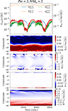 |
Fig. 11. Top: Time series of the magnetic energy. Bottom: Butterfly diagram showing the latitudinal structure time evolution of different axisymmetric magnetic field components averaged between the radii r = 5 and r = 6 km, and the axisymmetric radial magnetic field at the surface r = ro = 12 km. |
Quantitatively, we find  –2.1 × 10¹⁵ G for the models with N/Ωo ∈ [2, 10], which is very close to the maximum values
  –3 × 10¹⁵ G measured in the same models. The proximity to the instability threshold supports our interpretation. To characterise the time evolution of the intermittency, we measured its duty cycle αcyc; namely, the ratio of the time when the dynamo is active to the period of the cycle. We find that it varies between 0.38 and 0.66, with a tendency to decrease with N/Ωo as seen in Fig. 12. The same trend is observed for the period of these cycles Pcyc, which ranges between 3 s and 30 s. This is consistent with the fact that we get closer and closer to the dynamo threshold.
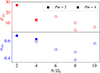 |
Fig. 12. Period of the cycle Pcyc (top) and the duty cycle αcyc (bottom) of the intermittent dynamo as a function of the input N/Ωo. Filled and empty markers represent self-sustained and transient dynamos, respectively. |
4. Application to magnetar formation
In this section, we apply our numerical results to the magnetar formation scenario proposed by Barrère et al. (2022), whose semi-analytical modelling was based on the formalism by Fuller et al. (2019). To this end, the magnetic field is converted into physical units by fixing the following parameters to typical values in PNSs: the PNS radius of ro = 12 km, mass of M = 1.4 M⊙ corresponding to a constant PNS density of ρ ∼ 3.8 × 10¹⁴ g cm−3, and Brunt-Väisälä frequency of N = 1 kHz. This value is a good proxy as it is consistent with 1D CCSNe simulations at 10 seconds after the core bounce (e.g. Hüdepohl 2014; Pascal et al. 2022). We note that it is lower than the one assumed in Barrère et al. (2022), which refers to earlier times. The accretion may be expected to heat the PNS surface (see e.g. Wijnands et al. 2017, for accretion on evolved NSs in X-ray binaries) and so change the value of N near the surface. Part of the energy of accretion heating will be radiated away by neutrino emission (Akaho et al. 2024). Improved models of PNS evolution similar to Hüdepohl (2014), Pascal et al. (2022), but including heating by fall-back accretion, would be needed for a more precise determination of the Brunt-Väisälä frequency. Finally, we note that all the simulations were performed with the same Ekman number E = 10−5. Therefore, fixing N implies that the diffusivities vary between the simulations.
Figure 13 shows the obtained magnetic field strength as a function of the angular frequency of the PNS surface, for the axisymmetric toroidal and poloidal components ( ,
,  , upper panel) and for the dipolar component Bdip (lower panel). The red markers correspond to the magnetic field measured in the simulations, while the blue markers correspond to the values extrapolated to q = 1 (as was assumed in Barrère et al. 2022). This plot can be compared to Fig. 5 in Barrère et al. (2022), the main difference being that here we define a low-field magnetar as a magnetar, with
  but Bdip < 4.4 × 10¹³ G. The magnetic field intensity show a similar trend with rotation frequency as was predicted by Barrère et al. (2022): the axisymmetric toroidal magnetic field increases as ∝Ω1.2 (∝Ω4/3 in Barrère et al. 2022), while the poloidal and dipolar components increase as ∝Ω2.4 (∝Ω8/3 in Barrère et al. 2022). This agreement is linked to the fact that the magnetic field in our numerical simulations aptly follows the Fuller et al. (2019) scaling law, as shown in the previous sections. The main difference is that the saturated magnetic field in our simulations is ∼17 times weaker than in the model in Barrère et al. (2022). This difference mainly comes from the assumptions in Barrère et al. (2022) of a stratification unaffected by diffusion and a dimensionless normalisation factor α = 1, while our simulations indicate α ≃ 0.01 (see Table 1).
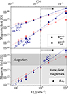 |
Fig. 13. Magnetic strength of the axisymmetric toroidal, |


The weaker magnetic field in our numerical simulations shifts the upper limit of the rotation period to form magnetar-like magnetic fields to P ≲ 6 ms (to be compared to P ≲ 28 ms in Barrère et al. 2022). This new limit corresponds to an accreted fall-back mass limit of M ≳ 5 × 10⁻² M⊙, which is higher than in Barrère et al. (2022) but still consistent with recent supernova simulations (see the discussion in Barrère et al. 2022). By assuming that all the rotational energy of the PNS is converted into kinetic energy of the explosion, the observations of SN remnants associated to magnetars constrained a minimum initial PNS rotation period of P0 ≳ 5 ms (Vink & Kuiper 2006). This value is close to our new constraint of the period upper limit to form magnetars through our scenario, which would leave only a small parameter space for the formation of magnetars by the Tayler-Spruit dynamo (5 ms < P < 6 ms). However, we argue that our simulations may underestimate the strength of magnetic fields that would be generated in a realistic PNS because of the high diffusivities used for numerical reasons (see Sect. 5.1).
For rotation periods longer than 6 ms, the magnetic dipole is too weak to form a classical magnetar, but the Tayler-Spruit dynamo still produces strong total magnetic fields above 1014 G. We suggest that these could correspond to the formation of low-dipolar field magnetars. Indeed, the observations of absorption lines in the X-ray spectra of low-field magnetars (Tiengo et al. 2013; Rodríguez Castillo et al. 2016) and 3D numerical simulations of magnetic field long-term evolution in NSs (Igoshev et al. 2021) suggest that such strength is enough to produce magnetar-like luminous activity. Furthermore, our recent simulations of NS magneto-thermal evolution confirm the link between the Tayler-Spruit dynamo and low-dipolar field magnetars (Igoshev et al. 2025).
5. Discussion
Here, we discuss the simplifications we used for the modelling of the PNS interior evolution: the diffusion processes (Sect. 5.1), the initial magnetic field (Sect. 5.2), the mechanism to force the differential rotation (Sect. 5.3), and the Boussinesq approximation (Sect. 5.4). In Sect. 5.5, we finally compare our results on the Tayler-Spruit dynamo (Barrère et al. 2023, this article) and the Tayler-Spruit dynamo obtained in other numerical simulations (Petitdemange et al. 2023; Daniel et al. 2023; Petitdemange et al. 2024).
5.1. Dependence on diffusion processes
As is usual in astrophysical fluid dynamics, one of the most important limitations of our simulations is that they are far from the realistic regime for the different diffusivities. This is particularly true for the magnetic Prandtl number Pm, which reaches Pm ∼ 1011, assuming a neutrino viscosity (Pm ∼ 104 assuming a shear viscosity) in PNSs ∼1010 s after the core bounce (see the section on supplementary materials in Barrère et al. 2023). The thermal diffusivity is also much larger than the resistivity in a PNS, which implies a small effective Brunt-Väisälä frequency of Neff = 2.2 × 10⁻⁸ N, assuming a neutrino viscosity (Neff = 8 × 10⁻⁴ N assuming a shear viscosity). The high-Pm regime and the alleviation of the stable stratification favour most likely the development of the dynamo and stronger magnetic fields. The extrapolation of our results to the high Pm regime is an important open question, as it is unclear whether the theoretical scalings will hold in this regime.
5.2. Initial magnetic field and dynamo threshold
The numerical simulations in this paper were initialised with a nearby saturated state, except for the simulation at N/Ωo = 0.1 (named ‘Ro0.75s’ in Table. C.1), which started from a strong axisymmetric toroidal field that is already unstable to the Tayler instability. Using the nearby saturated state has the advantage to follow more easily the dynamo branch through the parameter space without losing the dynamo despite its subcritical nature (see e.g. Raynaud & Tobias 2016; Petitdemange et al. 2023). Starting from a strong axisymmetric toroidal field (Λν ∼ 10), which allows the fluid to become unstable, in line with the Tayler instability, and causes it to skip the initial growth phase to reach the critical strength  (Eq. (23)). We have checked in a few cases that the saturated state does not depend on the initial magnetic field as long as the dynamo operates. An example is given in Appendix A, in which the numerical simulations initialised with a pure magnetic dipole or a strong toroidal field saturate both at the same magnetic energies.
Furthermore, as discussed in the previous section, the resistivity in our simulations is much larger than in a realistic PNS. As a consequence, the critical magnetic field for the Tayler instability and so, the dynamo threshold, is more difficult to reach in our simulations ( –2.1 × 10¹⁵ G) than in a PNS (
 ; see Sect. 2.2. of Barrère et al. 2022); in the latter, the threshold could be easily reached by shearing a magnetic dipole stemming from the progenitor star. Moreover, Barrère et al. (2022) predicted that the growth of the Tayler mode becomes significant (i.e. faster than the growth due to the shear) only when the toroidal field is two orders of magnitude stronger than both the instability threshold and the radial magnetic field (for Bϕ ∼ 5 × 10¹⁴ G). This justifies the use of a strong toroidal field as an initial condition for our simulations.
5.3. Forcing of the differential rotation
To force the differential rotation, we chose to use a spherical Taylor-Couette configuration, in which a constant rotation rate is imposed on both inner and outer spheres. In this set-up, the rotation profile is free to evolve as the angular momentum is transported by turbulence and large-scale magnetic fields. The imposed rotation of the outer sphere is meant to roughly mimics the maintenance of the surface rotation due to fall-back accretion, once the PNS surface is already spun up significantly. We note, however, that this idealised boundary condition neglects the time evolution of the fall-back accretion. Therefore, the rotation profile evolution does not describe the beginning of the accretion, when the surface is spun up and the differential rotation (initially concentrated close to the surface) is transported in the PNS interior.
Maintaining the rotation on both spheres allows us to inject energy into the flow and try to control the shear rate. As noted in Sect. 3.4 and further quantified in Appendix B, the stable stratification does end up significantly changing the shear rate. This complicates the measure of the respective scaling exponents with N/Ωo and q independently. In addition, we observe in Fig. 2 that most of the shear is concentrated closer and closer to the inner sphere. As confirmed by our simulations, this restricts significantly the domain in which the Tayler-Spruit dynamo can operate and act to make the dynamo more difficult to sustain. Thus, to investigate stronger stratification regimes, it will be necessary to change the forcing method and perhaps opt for a volumetric forcing, as applied, for instance, by Meduri et al. (2024).
Finally, strongly asymmetric and localised accretion could also lead to angle dependent differential rotation on the PNS surface, which might change the magnetic field geometry near the surface. Therefore, more realistic outer boundary conditions to force differential rotation could be implemented in future work by using the results of 3D MHD simulations of accretion. Moreover, the formation of mounds due to accretion may bury the magnetic field and so reduce the magnetic dipole (Priymak et al. 2011; Suvorov & Melatos 2020), but MHD instabilities in the mound may strongly reduce the burial efficiency for large accreted masses (Mukherjee et al. 2013; Mukherjee 2017).
5.4. Validity of the Boussinesq approximation
To model the PNS interior, we used the Boussinesq approximation, which reduces the numerical cost and allows us to produce a few tens of models to better understand the physics of the Tayler-Spruit dynamo. Despite the importance of the density gradient, this approximation is reasonable in the case of PNS interior:
-
(i)
The sound speed is close to the speed of light cs ∼ 1010 cm s−1 (Hüdepohl 2014; Pascal 2021, private communication), so vA/cs ≲ vϕ/cs ≲ 10−2, where va ≡ roωA and vϕ are the typical Alfvén and azimuthal speeds.
-
(ii)
The density perturbation associated to the buoyancy term is small compared to the PNS mean density: δρ/ρ = θN2/g ≲ 9 × 10⁻², with N = 103 s−1, g ∼ GM/ro ∼ 1.3 × 1013 cm s−2, and θ ≲ ro is the buoyancy variable (Eq. 6).
The impact of density gradient on the Tayler-Spruit dynamo has never been investigated so far in numerical simulations. According to 1D CCSN models, ∼10 s after the core bounce, the PNS interior density is almost constant in the core but drops in the ∼2 km below the surface. This may change the results and motivates future work to consider more realistic PNS density profiles. Reboul-Salze et al. (2022) compare the numerical results of the MRI in a PNS with and without a density gradient. The main differences are the appearance of a reversing axisymmetric toroidal magnetic field and a magnetic field that is concentrated in low-density regions, while the magnetic field strength remains similar.
5.5. Comparison with other numerical models
In the literature, only a few other studies have carried out numerical investigations of the Tayler-Spruit dynamo (Petitdemange et al. 2023, 2024; Daniel et al. 2023). The main difference between our set-up and theirs is the opposite shear; namely, in their set-up, the inner boundary rotates faster than the outer one. As we have, they did find a subcritical bifurcation at the Tayler instability threshold to a self-sustained state with a dominant axisymmetric toroidal magnetic field. However, many differences have been noted:
-
The generated magnetic structure in their simulations has a smaller scale and is localized near the inner sphere in the equatorial plane. The impact of stable stratification on the length scale of these modes may deserve a deeper analysis. It is still unclear why a dynamo-generated magnetic field is so different for positive and negative shear, although existing theories of the Tayler-Spruit dynamo do not depend on the sign of the shear (Spruit 2002; Fuller et al. 2019). It would be interesting to investigate whether it could be related to the potential interaction with the magnetorotational instability (which is stable for positive shear, but potentially unstable for negative shear).
-
As in Barrère et al. (2023), a hemispherical dynamo solution is also found by Petitdemange et al. (2024) as they move from a laminar dynamo solution to the strong Tayler-Spruit dynamo by increasing N/Ωo. However, they do not find bistability between the hemispherical and the strong solutions as in Barrère et al. (2023).
-
While the dipolar and hemispherical dynamos we found in Barrère et al. (2023) are in good agreement with the predictions of Fuller et al. (2019) and Spruit (2002), respectively, all their models, including those of the hemispherical solution, are in agreement with the analytical model of Spruit (2002).
Therefore, the few numerical studies of the Tayler-Spruit dynamo indicate a much more complex physics than anticipated analytically, with the existence of a wide variety of dynamo solutions. So far, only Daniel et al. (2023) propose a non-linear model of the subcritical transition to the Tayler-Spruit dynamo of Petitdemange et al. (2023). To include the other solutions we discovered, we must further investigate the dynamics of the dynamo using tools from dynamic system theory.
6. Conclusions
6.1. Summary
Following our previous study Barrère et al. (2023) of the Tayler-Spruit dynamo with a fixed ratio of rotation to Brunt-Väisälä frequency, we performed numerical simulations of the dipolar Tayler-Spruit dynamo to investigate its dependence on the level of stratification. The main results can be summarized as follows:
-
We find self-sustained Tayler-Spruit dynamos for stratifications up to N/Ωo = 4 (and up to N/Ωo = 10 for transient dynamos). The dynamo also becomes intermittent as the saturated
 is close to the Tayler instability threshold for N/Ωo ≥ 2.
 -
We observed a good agreement with the scaling laws of Fuller et al. (2019) for large-scale magnetic fields and the angular momentum transport, the latter of which is dominated by Maxwell torques.
-
With increasing N/Ωo, the Tayler modes have reduced radial length scales as expected but their energy decreases faster than theoretically predicted, which may indicate an underestimation of the turbulent dissipation by the analytical models.
-
By measuring an approximate mixing diffusivity, we also determined the efficiency of the mixing process due to the Tayler-Spruit dynamo. We find that mixing is far less efficient than the angular momentum transport, as analytically predicted.
-
Finally, as in the study of Fuller et al. (2019), we have defined a dimensionless normalisation factor α parameterising the scaling law of
 and numerically constrained its value to α ∼ 10−2. Therefore, the large-scale magnetic fields in our simulations are weaker than theoretically foreseen.
Applying these results to the magnetar formation scenario of Barrère et al. (2022), the rotation threshold to form classical magnetar-like dipoles is found to be more constraining than derived in Barrère et al. (2022), with a rotation period of P ≲ 6 ms (compared to P ≲ 28 ms in Barrère et al. 2022). This value corresponds to an accreted fall-back mass of M ≳ 5 × 10⁻² M⊙, which is still reasonable according to CCSN simulations (e.g. Sukhbold et al. 2016, 2018; Chan et al. 2020; Janka et al. 2022). This new constraint is close to the minimum initial PNS period derived from the kinetic energy of SN remnants associated to magnetars (Vink & Kuiper 2006), suggesting some tension with observations. We note, however, that these conclusions are likely to be quantitatively affected by a number of simplifications made in our approach and discussed in Sect. 5. In particular, the too high diffusivities of our simulations compared to a realistic PNS regime may lead us to underestimate the magnetic field intensity, which could alleviate the tension with observations for the formation of classical magnetars (Sect. 5.1).
Furthermore, the total magnetic field remains very strong (≳1014 G) for slow rotation periods (≲60 ms), which makes our scenario a promising mechanism behind the formation of magnetars with weaker magnetic dipoles, as demonstrated by our recent numerical study (Igoshev et al. 2025).
6.2. Long-term evolution of the magnetic field
After ∼100 s, the fall-back accretion becomes too weak to maintain the differential rotation in the PNS. The newly formed strong large-scale magnetic fields transport the angular momentum efficiently, which damps the differential rotation and the dynamo will eventually stop. The magnetic field is expected to enter a relaxation phase in which its structure changes to reach a stable configuration. The exact shape of this magnetic field is still an open question and, more generally, the magnetic relaxation problem in astrophysics remains a matter of debate (e.g. Braithwaite 2006; Duez & Mathis 2010; Duez et al. 2010; Akgün et al. 2013; Becerra et al. 2022a,b). It is, however, widely acknowledged that the magnetic configuration is complex, mixing both large-scale poloidal and toroidal components. Thus, 3D numerical simulations including thermal and density stratifications and rotation are required to investigate this stage of the PNS evolution.
On longer timescales of ∼1–100 kyr, the remaining strong toroidal magnetic fields located in the NS crust are prone to Hall diffusion and instability (Rheinhardt & Geppert 2002), which modifies their structures and so can influence the magnetar emission. In a recent numerical study (Igoshev et al. 2025), we investigated the NS magneto-thermal evolution of a NS harbouring a magnetic field generated by the Tayler-Spruit dynamo. The results suggest that the formation of hot spots at the footpoint of 1014 G-magnetic arches explains the observational properties of low-dipolar field magnetars. Moreover, the strong magnetic field-induced stresses cause failures or plastic deformations, which are strongly suspected to explain the origin of magnetar bursts (e.g. Thompson & Duncan 1995; Perna & Pons 2011; Lander et al. 2015; Lander & Gourgouliatos 2019). This investigation strongly motivates further studies that could also include the relaxation of the dynamo-generated magnetic field to a stable configuration before the PNS becomes a cooled stable NS.
6.3. Interaction with a remaining fall-back disc
The magnetic dipole generated by the dipolar Tayler-Spruit dynamo may not be strong enough to spin the magnetar down to the observed 8–12 s via the magnetic spin-down mechanism. A good alternative would be the propeller mechanism (e.g. Gompertz et al. 2014; Beniamini et al. 2019; Lin et al. 2021; Ronchi et al. 2022). This operates when the magnetosphere is large enough to interact with the remaining fall-back disc, that is, when the Alfvén radius is larger than the corotation radius. In the propeller regime, the inner disk matter is accelerated to super-Keplerian velocity, which produces an outflow and so an angular momentum transfer from the magnetar to the disc. If this mechanism is operating in some magnetars, the magnetic dipole (which is inferred from the values of the NS rotation period and its associated derivative) will be overestimated. Our model of PNS-disc interaction in Igoshev et al. (2025) indicates that a 1012 G-magnetic dipole is sufficient to explain the rotation of low-dipolar field magnetars. This implies an overestimation of ∼40 of the magnetic dipole by the classical magnetic dipole spin-down formula. It thus fosters numerical studies of the fall-back matter in 3D simulations of CCSNe and investigations on the evolution of the potential remaining disc. This will help constrain which progenitors are the best candidates to form magnetars via our fall-back scenario.
6.4. Implications for stellar physics
Our findings are also of importance with respect to studies of stellar radiative zones. Indeed, the scaling laws and the dimensionless normalisation factor α derived from our simulations could be implemented in 1D stellar evolution codes. Evolution models using the prescriptions of Fuller et al. (2019) have already been computed for sub-giant and red giant stars but with larger values of α ∼ 0.25 − 1. These studies find a strong flattening of the rotation profile and conclude that the prescribed Tayler-Spruit dynamo cannot explain both rotation profiles of sub-giant and red giant stars (Eggenberger et al. 2019b), which suggests that different angular momentum transport mechanisms occur during these two phases (Eggenberger et al. 2019a). Future asteroseismic measurements of the magnetic fields in stellar interiors obtained with PLATO will be crucial in clarifying the question of the transport mechanisms. Although the first measurements of magnetic fields in some red giant cores suggest a strong fossil field (Li et al. 2022, 2023; Deheuvels et al. 2023), it will be essential to infer the asteroseismic signature of magnetic fields generated by the simulated Tayler-Spruit dynamos for such future observations. Evolution models including MHD instabilities effects have also been performed in the case of massive stars to constrain the rotation rate of the remaining PNS or black hole (Griffiths et al. 2022; Fuller & Lu 2022). They suggest that the angular momentum transport by MHD instabilities is significant in every stage of the massive star evolution. This highlights the importance of performing 3D anelastic simulations with realistic background profiles of radiative zones at different evolutionary stages to better constrain the angular momentum transport and infer more robust rotation rates for stellar cores.
Commit 2266201a5 on https://github.com/magic-sph/magic
For the choice of these definitions, see Gubbins & Zhang (1993).
Acknowledgments
We thank the referee for their constructive comments that helped us improve the clarity of the manuscript. This work was supported by the European Research Council (MagBURST grant 715368), and the PNPS and PNHE programs of CNRS/INSU, co-funded by CEA and CNES. Numerical simulations have been carried out at the CINES on the Jean-Zay supercomputer and at the TGCC on the supercomputer IRENE-ROME (DARI project A130410317).
References
- Akaho, R., Nagakura, H., & Foglizzo, T. 2024, ApJ, 960, 116 [NASA ADS] [CrossRef] [Google Scholar]
- Akgün, T., Reisenegger, A., Mastrano, A., & Marchant, P. 2013, MNRAS, 433, 2445 [Google Scholar]
- Barcilon, V., & Pedlosky, J. 1967a, J. Fluid Mech., 29, 1 [Google Scholar]
- Barcilon, V., & Pedlosky, J. 1967b, J. Fluid Mech., 29, 673 [NASA ADS] [CrossRef] [Google Scholar]
- Barcilon, V., & Pedlosky, J. 1967c, J. Fluid Mech., 29, 609 [NASA ADS] [CrossRef] [Google Scholar]
- Barrère, P., Guilet, J., Reboul-Salze, A., Raynaud, R., & Janka, H. T. 2022, A&A, 668, A79 [NASA ADS] [CrossRef] [EDP Sciences] [Google Scholar]
- Barrère, P., Guilet, J., Raynaud, R., & Reboul-Salze, A. 2023, MNRAS, 526, L88 [CrossRef] [Google Scholar]
- Becerra, L., Reisenegger, A., Valdivia, J. A., & Gusakov, M. 2022a, MNRAS, 517, 560 [NASA ADS] [CrossRef] [Google Scholar]
- Becerra, L., Reisenegger, A., Valdivia, J. A., & Gusakov, M. E. 2022b, MNRAS, 511, 732 [NASA ADS] [CrossRef] [Google Scholar]
- Beniamini, P., Hotokezaka, K., van der Horst, A., & Kouveliotou, C. 2019, MNRAS, 487, 1426 [NASA ADS] [CrossRef] [Google Scholar]
- Bochenek, C. D., Ravi, V., Belov, K. V., et al. 2020, Nature, 587, 59 [NASA ADS] [CrossRef] [Google Scholar]
- Boscarino, S., Pareschi, L., & Russo, G. 2013, SIAM J. Sci. Comput., 35, A22 [CrossRef] [Google Scholar]
- Braithwaite, J. 2006, A&A, 449, 451 [NASA ADS] [CrossRef] [EDP Sciences] [Google Scholar]
- Bugli, M., Guilet, J., Obergaulinger, M., Cerdá-Durán, P., & Aloy, M. A. 2020, MNRAS, 492, 58 [NASA ADS] [CrossRef] [Google Scholar]
- Bugli, M., Guilet, J., & Obergaulinger, M. 2021, MNRAS, 507, 443 [NASA ADS] [CrossRef] [Google Scholar]
- Bugli, M., Guilet, J., Foglizzo, T., & Obergaulinger, M. 2023, MNRAS, 520, 5622 [NASA ADS] [CrossRef] [Google Scholar]
- Burrows, A., Dessart, L., Livne, E., Ott, C. D., & Murphy, J. 2007, ApJ, 664, 416 [NASA ADS] [CrossRef] [Google Scholar]
- Cantiello, M., Mankovich, C., Bildsten, L., Christensen-Dalsgaard, J., & Paxton, B. 2014, ApJ, 788, 93 [Google Scholar]
- Chan, C., Müller, B., & Heger, A. 2020, MNRAS, 495, 3751 [NASA ADS] [CrossRef] [Google Scholar]
- CHIME/FRB Collaboration (Andersen, B. C., et al.) 2020, Nature, 58, 7 [Google Scholar]
- Coti Zelati, F., Rea, N., Pons, J. A., Campana, S., & Esposito, P. 2018, MNRAS, 474, 961 [NASA ADS] [CrossRef] [Google Scholar]
- Coti Zelati, F., Borghese, A., Rea, N., et al. 2021, ATel, 14674, 1 [NASA ADS] [Google Scholar]
- Daniel, F., Petitdemange, L., & Gissinger, C. 2023, Phys. Rev. Fluids, 8, 123701 [NASA ADS] [CrossRef] [Google Scholar]
- Deheuvels, S., Doğan, G., Goupil, M. J., et al. 2014, A&A, 564, A27 [NASA ADS] [CrossRef] [EDP Sciences] [Google Scholar]
- Deheuvels, S., Ballot, J., Beck, P. G., et al. 2015, A&A, 580, A96 [NASA ADS] [CrossRef] [EDP Sciences] [Google Scholar]
- Deheuvels, S., Li, G., Ballot, J., & Lignières, F. 2023, A&A, 670, L16 [NASA ADS] [CrossRef] [EDP Sciences] [Google Scholar]
- den Hartogh, J. W., Eggenberger, P., & Deheuvels, S. 2020, A&A, 634, L16 [NASA ADS] [CrossRef] [EDP Sciences] [Google Scholar]
- Dessart, L., Burrows, A., Livne, E., & Ott, C. D. 2008, ApJ, 673, L43 [NASA ADS] [CrossRef] [Google Scholar]
- Dessart, L., Hillier, D. J., Waldman, R., Livne, E., & Blondin, S. 2012, MNRAS, 426, L76 [NASA ADS] [CrossRef] [Google Scholar]
- Drout, M. R., Soderberg, A. M., Gal-Yam, A., et al. 2011, ApJ, 741, 97 [NASA ADS] [CrossRef] [Google Scholar]
- Duez, V., & Mathis, S. 2010, A&A, 517, A58 [NASA ADS] [CrossRef] [EDP Sciences] [Google Scholar]
- Duez, V., Braithwaite, J., & Mathis, S. 2010, ApJ, 724, L34 [Google Scholar]
- Duncan, R. C., & Thompson, C. 1992, ApJ, 392, L9 [Google Scholar]
- Eggenberger, P., Maeder, A., & Meynet, G. 2005, A&A, 440, L9 [NASA ADS] [CrossRef] [EDP Sciences] [Google Scholar]
- Eggenberger, P., Deheuvels, S., Miglio, A., et al. 2019a, A&A, 621, A66 [NASA ADS] [CrossRef] [EDP Sciences] [Google Scholar]
- Eggenberger, P., den Hartogh, J. W., Buldgen, G., et al. 2019b, A&A, 631, L6 [NASA ADS] [CrossRef] [EDP Sciences] [Google Scholar]
- Evans, W. D., Klebesadel, R. W., Laros, J. G., et al. 1980, ApJ, 237, L7 [NASA ADS] [CrossRef] [Google Scholar]
- Ferrario, L., & Wickramasinghe, D. 2006, MNRAS, 367, 1323 [NASA ADS] [CrossRef] [Google Scholar]
- Fuller, J., & Lu, W. 2022, MNRAS, 511, 3951 [NASA ADS] [CrossRef] [Google Scholar]
- Fuller, J., Piro, A. L., & Jermyn, A. S. 2019, MNRAS, 485, 3661 [NASA ADS] [Google Scholar]
- Gastine, T., & Wicht, J. 2012, Icarus, 219, 428 [Google Scholar]
- Gaurat, M., Jouve, L., Lignières, F., & Gastine, T. 2015, A&A, 580, A103 [NASA ADS] [CrossRef] [EDP Sciences] [Google Scholar]
- Gehan, C., Mosser, B., Michel, E., Samadi, R., & Kallinger, T. 2018, A&A, 616, A24 [NASA ADS] [CrossRef] [EDP Sciences] [Google Scholar]
- Gompertz, B., & Fruchter, A. 2017, ApJ, 839, 49 [NASA ADS] [CrossRef] [Google Scholar]
- Gompertz, B. P., O’Brien, P. T., & Wynn, G. A. 2014, MNRAS, 438, 240 [NASA ADS] [CrossRef] [Google Scholar]
- Goossens, M., & Tayler, R. J. 1980, MNRAS, 193, 833 [NASA ADS] [Google Scholar]
- Gotz, D., Israel, G. L., Mereghetti, S., et al. 2006, ATel, 953, 1 [NASA ADS] [Google Scholar]
- Griffiths, A., Eggenberger, P., Meynet, G., Moyano, F., & Aloy, M.-Á. 2022, A&A, 665, A147 [NASA ADS] [CrossRef] [EDP Sciences] [Google Scholar]
- Gubbins, D., & Zhang, K. 1993, Phys. Earth Planet. Inter., 75, 225 [Google Scholar]
- Guilet, J., Müller, E., & Janka, H.-T. 2015, MNRAS, 447, 3992 [NASA ADS] [CrossRef] [Google Scholar]
- Guilet, J., Reboul-Salze, A., Raynaud, R., Bugli, M., & Gallet, B. 2022, MNRAS, 516, 4346 [NASA ADS] [CrossRef] [Google Scholar]
- Hu, R.-Y., & Lou, Y.-Q. 2009, MNRAS, 396, 878 [NASA ADS] [CrossRef] [Google Scholar]
- Hüdepohl, L. 2014, Ph.D. Thesis, Technical University of Munich, Germany [Google Scholar]
- Hurley, K., Cline, T., Mazets, E., et al. 1999, Nature, 397, 41 [NASA ADS] [CrossRef] [Google Scholar]
- Hurley, K., Boggs, S. E., Smith, D. M., et al. 2005, Nature, 434, 1098 [NASA ADS] [CrossRef] [Google Scholar]
- Igoshev, A. P., Hollerbach, R., Wood, T., & Gourgouliatos, K. N. 2021, Nat. Astron., 5, 145 [Google Scholar]
- Igoshev, A., Barrère, P., Raynaud, R., et al. 2025, arXiv e-prints [arXiv:2501.04768] [Google Scholar]
- Inserra, C., Smartt, S. J., Jerkstrand, A., et al. 2013, ApJ, 770, 128 [NASA ADS] [CrossRef] [Google Scholar]
- Janka, H.-T., Wongwathanarat, A., & Kramer, M. 2022, ApJ, 926, 9 [NASA ADS] [CrossRef] [Google Scholar]
- Ji, S., Fuller, J., & Lecoanet, D. 2023, MNRAS, 521, 5372 [NASA ADS] [CrossRef] [Google Scholar]
- Kasen, D., & Bildsten, L. 2010, ApJ, 717, 245 [NASA ADS] [CrossRef] [Google Scholar]
- Kiuchi, K., Reboul-Salze, A., Shibata, M., & Sekiguchi, Y. 2024, Nat. Astron., 8, 298 [Google Scholar]
- Kouveliotou, C., Fishman, G. J., Meegan, C. A., et al. 1994, Nature, 368, 125 [CrossRef] [Google Scholar]
- Kuroda, T., Arcones, A., Takiwaki, T., & Kotake, K. 2020, ApJ, 896, 102 [NASA ADS] [CrossRef] [Google Scholar]
- Lander, S. K., & Gourgouliatos, K. N. 2019, MNRAS, 486, 4130 [NASA ADS] [CrossRef] [Google Scholar]
- Lander, S. K., Andersson, N., Antonopoulou, D., & Watts, A. L. 2015, MNRAS, 449, 2047 [NASA ADS] [CrossRef] [Google Scholar]
- Li, G., Deheuvels, S., Ballot, J., & Lignières, F. 2022, Nature, 610, 43 [NASA ADS] [CrossRef] [Google Scholar]
- Li, G., Deheuvels, S., Li, T., Ballot, J., & Lignières, F. 2023, A&A, 680, A26 [NASA ADS] [CrossRef] [EDP Sciences] [Google Scholar]
- Lin, W., Wang, X., Wang, L., & Dai, Z. 2021, ApJ, 914, L2 [NASA ADS] [CrossRef] [Google Scholar]
- Lü, H.-J., & Zhang, B. 2014, ApJ, 785, 74 [CrossRef] [Google Scholar]
- Ma, L., & Fuller, J. 2019, MNRAS, 488, 4338 [NASA ADS] [CrossRef] [Google Scholar]
- Makarenko, E. I., Igoshev, A. P., & Kholtygin, A. F. 2021, MNRAS, 504, 5813 [NASA ADS] [CrossRef] [Google Scholar]
- Martin, J., Rea, N., Torres, D. F., & Papitto, A. 2014, MNRAS, 444, 2910 [NASA ADS] [CrossRef] [Google Scholar]
- Masada, Y., Takiwaki, T., & Kotake, K. 2022, ApJ, 924, 75 [NASA ADS] [CrossRef] [Google Scholar]
- Meduri, D. G., Jouve, L., & Lignières, F. 2024, A&A, 683, A12 [NASA ADS] [CrossRef] [EDP Sciences] [Google Scholar]
- Mereghetti, S., Savchenko, V., Ferrigno, C., et al. 2020, ApJ, 898, L29 [Google Scholar]
- Metzger, B. D., Giannios, D., Thompson, T. A., Bucciantini, N., & Quataert, E. 2011, MNRAS, 413, 2031 [Google Scholar]
- Metzger, B. D., Beniamini, P., & Giannios, D. 2018, ApJ, 857, 95 [NASA ADS] [CrossRef] [Google Scholar]
- Mosser, B., Goupil, M. J., Belkacem, K., et al. 2012, A&A, 548, A10 [NASA ADS] [CrossRef] [EDP Sciences] [Google Scholar]
- Mösta, P., Richers, S., Ott, C. D., et al. 2014, ApJ, 785, L29 [CrossRef] [Google Scholar]
- Mukherjee, D. 2017, JA&A, 38, 48 [NASA ADS] [Google Scholar]
- Mukherjee, D., Bhattacharya, D., & Mignone, A. 2013, MNRAS, 435, 718 [Google Scholar]
- Nicholl, M., Smartt, S. J., Jerkstrand, A., et al. 2013, Nature, 502, 346 [NASA ADS] [CrossRef] [Google Scholar]
- Nomoto, K., Maeda, K., Tanaka, M., & Suzuki, T. 2011, Astrophys. Science Sci., 336, 129 [NASA ADS] [CrossRef] [Google Scholar]
- Obergaulinger, M., & Aloy, M. Á. 2020, MNRAS, 492, 4613 [Google Scholar]
- Obergaulinger, M., & Aloy, M. Á. 2021, MNRAS, 503, 4942 [NASA ADS] [CrossRef] [Google Scholar]
- Obergaulinger, M., & Aloy, M. Á. 2022, MNRAS, 512, 2489 [NASA ADS] [CrossRef] [Google Scholar]
- Obergaulinger, M., Cerdá-Durán, P., Müller, E., & Aloy, M. A. 2009, A&A, 498, 241 [NASA ADS] [CrossRef] [EDP Sciences] [Google Scholar]
- Olausen, S. A., & Kaspi, V. M. 2014, ApJS, 212, 6 [Google Scholar]
- Pascal, A. 2021, Theses, Université Paris sciences et lettres, France [Google Scholar]
- Pascal, A., Novak, J., & Oertel, M. 2022, MNRAS, 511, 356 [NASA ADS] [CrossRef] [Google Scholar]
- Perna, R., & Pons, J. A. 2011, ApJ, 727, L51 [NASA ADS] [CrossRef] [Google Scholar]
- Petitdemange, L., Marcotte, F., & Gissinger, C. 2023, Science, 379, 300 [NASA ADS] [CrossRef] [Google Scholar]
- Petitdemange, L., Marcotte, F., Gissinger, C., & Daniel, F. 2024, A&A, 681, A75 [NASA ADS] [CrossRef] [EDP Sciences] [Google Scholar]
- Philidet, J., Gissinger, C., Lignières, F., & Petitdemange, L. 2020, Geophys. Astrophys. Fluid Dyn., 114, 336 [CrossRef] [Google Scholar]
- Priymak, M., Melatos, A., & Payne, D. J. B. 2011, MNRAS, 417, 2696 [Google Scholar]
- Raynaud, R., & Tobias, S. M. 2016, J. Fluid Mech., 799, R6 [NASA ADS] [CrossRef] [Google Scholar]
- Raynaud, R., Guilet, J., Janka, H.-T., & Gastine, T. 2020, Sci. Adv., 6, eaay2732 [NASA ADS] [CrossRef] [Google Scholar]
- Raynaud, R., Cerdá-Durán, P., & Guilet, J. 2022, MNRAS, 509, 3410 [Google Scholar]
- Rea, N., Esposito, P., Turolla, R., et al. 2010, Science, 330, 944 [NASA ADS] [CrossRef] [Google Scholar]
- Rea, N., Israel, G. L., Esposito, P., et al. 2012, ApJ, 754, 27 [NASA ADS] [CrossRef] [Google Scholar]
- Rea, N., Israel, G. L., Pons, J. A., et al. 2013, ApJ, 770, 65 [NASA ADS] [CrossRef] [Google Scholar]
- Rea, N., Viganò, D., Israel, G. L., Pons, J. A., & Torres, D. F. 2014, ApJ, 781, L17 [NASA ADS] [CrossRef] [Google Scholar]
- Reboul-Salze, A., Guilet, J., Raynaud, R., & Bugli, M. 2021, A&A, 645, A109 [NASA ADS] [CrossRef] [EDP Sciences] [Google Scholar]
- Reboul-Salze, A., Guilet, J., Raynaud, R., & Bugli, M. 2022, A&A, 667, A94 [NASA ADS] [CrossRef] [EDP Sciences] [Google Scholar]
- Rembiasz, T., Obergaulinger, M., Cerdá-Durán, P., Aloy, M.-Á., & Müller, E. 2017, ApJS, 230, 18 [Google Scholar]
- Rheinhardt, M., & Geppert, U. 2002, Phys. Rev. Lett., 88, 101103 [Google Scholar]
- Rodríguez Castillo, G. A., Israel, G. L., Tiengo, A., et al. 2016, MNRAS, 456, 4145 [CrossRef] [Google Scholar]
- Ronchi, M., Rea, N., Graber, V., & Hurley-Walker, N. 2022, ApJ, 934, 184 [NASA ADS] [CrossRef] [Google Scholar]
- Schaeffer, N. 2013, Geochem. Geophys. Geosyst., 14, 751 [NASA ADS] [CrossRef] [Google Scholar]
- Schneider, F. R. N., Ohlmann, S. T., Podsiadlowski, P., et al. 2019, Nature, 574, 211 [Google Scholar]
- Shenar, T., Wade, G. A., Marchant, P., et al. 2023, Science, 381, 761 [NASA ADS] [CrossRef] [Google Scholar]
- Skoutnev, V. A., & Beloborodov, A. M. 2024a, ApJ, 974, 290 [NASA ADS] [CrossRef] [Google Scholar]
- Skoutnev, V. A., & Beloborodov, A. M. 2024b, arXiv e-prints [arXiv:2411.08492] [Google Scholar]
- Spruit, H. C. 1999, A&A, 349, 189 [NASA ADS] [Google Scholar]
- Spruit, H. C. 2002, A&A, 381, 923 [CrossRef] [EDP Sciences] [Google Scholar]
- Stockinger, G., Janka, H. T., Kresse, D., et al. 2020, MNRAS, 496, 2039 [Google Scholar]
- Sukhbold, T., Ertl, T., Woosley, S. E., Brown, J. M., & Janka, H. T. 2016, ApJ, 821, 38 [NASA ADS] [CrossRef] [Google Scholar]
- Sukhbold, T., Woosley, S. E., & Heger, A. 2018, ApJ, 860, 93 [NASA ADS] [CrossRef] [Google Scholar]
- Suvorov, A. G., & Melatos, A. 2020, MNRAS, 499, 3243 [NASA ADS] [CrossRef] [Google Scholar]
- Svinkin, D., Frederiks, D., Hurley, K., et al. 2021, Nature, 589, 211 [NASA ADS] [CrossRef] [Google Scholar]
- Takiwaki, T., Kotake, K., & Sato, K. 2009, ApJ, 691, 1360 [NASA ADS] [CrossRef] [Google Scholar]
- Tayler, R. J. 1973, MNRAS, 161, 365 [CrossRef] [Google Scholar]
- Thompson, C., & Duncan, R. C. 1993, ApJ, 408, 194 [NASA ADS] [CrossRef] [Google Scholar]
- Thompson, C., & Duncan, R. C. 1995, MNRAS, 275, 255 [Google Scholar]
- Tiengo, A., Esposito, P., Mereghetti, S., et al. 2013, Nature, 500, 312 [CrossRef] [Google Scholar]
- Tsuzuki, Y., Totani, T., Hu, C.-P., & Enoto, T. 2024, MNRAS, 530, 1885 [NASA ADS] [CrossRef] [Google Scholar]
- Vink, J., & Kuiper, L. 2006, MNRAS, 370, L14 [NASA ADS] [CrossRef] [Google Scholar]
- White, C. J., Burrows, A., Coleman, M. S. B., & Vartanyan, D. 2022, ApJ, 926, 111 [NASA ADS] [CrossRef] [Google Scholar]
- Wicht, J. 2002, Phys. Earth Planet. Inter., 132, 281 [Google Scholar]
- Wijnands, R., Degenaar, N., & Page, D. 2017, JA&A, 38, 49 [Google Scholar]
- Woosley, S. E. 2010, ApJ, 719, L204 [NASA ADS] [CrossRef] [Google Scholar]
- Woosley, S. E., & Bloom, J. S. 2006, ARA&A, 44, 507 [Google Scholar]
- Younes, G., Kouveliotou, C., Jaodand, A., et al. 2017, ApJ, 847, 85 [NASA ADS] [CrossRef] [Google Scholar]
- Zahn, J. P., Brun, A. S., & Mathis, S. 2007, A&A, 474, 145 [NASA ADS] [CrossRef] [EDP Sciences] [Google Scholar]
- Zhang, B., & Mészáros, P. 2001, ApJ, 552, L35 [CrossRef] [Google Scholar]
- Zhou, P., Vink, J., Safi-Harb, S., & Miceli, M. 2019, A&A, 629, A51 [NASA ADS] [CrossRef] [EDP Sciences] [Google Scholar]
- Zhu, W., Xu, H., Zhou, D., et al. 2023, Sci. Adv., 9, eadf6198 [NASA ADS] [CrossRef] [Google Scholar]
Appendix A: Tayler-Spruit dynamo from a different initial magnetic field
To check whether the saturated state of the Tayler-Spruit dynamo depends on the initial magnetic field, we produced an additional run using the same parameters as the run ‘Ro0.75s’ (E = 1 × 10⁻⁵, Pr = 0.1, Pm = 1, N/Ωo = 0.1) but with an initial purely dipolar magnetic field. Figure A.1 shows the time series of the axisymmetric toroidal, axisymmetric poloidal, and dipolar components of the magnetic energy densities for the runs with an initial magnetic dipole (stable to Tayler instability, plot on the left) and an initial strong axisymmetric azimuthal magnetic field (unstable to the Tayler instability, plot on the right). Both times series show the same saturated energies despite the different initialisations. The only difference in the evolution of magnetic field is the existence of an initial short shearing phase in which the toroidal component grows for the case of an initial magnetic dipole.
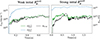 |
Fig. A.1. Time series of the axisymmetric toroidal ( |


Appendix B: Measure of the shear rate
The differential rotation is characterized by a dimensionless shear rate q = r∂rlnΩ. We define an effective shear rate based on the time average of the radial rotation profile in the saturated state at the colatitude of θ = π/8 rad. We measured an average slope in the range of radii where half of the Tayler mode energy (approximated by the latitudinal magnetic energy EBθ) is concentrated around its maximum. We chose this particular method because this range of radii is the region where the dynamo occurs. The measures are displayed in Fig. B.1 (red plot) along with other measures made with different methods. Whatever the method used, we see that all the measures follow the same trend with an increase of q ∝ N until N/Ωo = 4 after which the values of q stay almost constant.
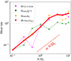 |
Fig. B.1. Shear rates q measured locally in the simulations as a function of N/Ωo. The different colours represent distinct methods to measure q: slope in the rotation profile between 3.2 and 4 km (pink), q at the maximum of |

Appendix C: List of models
Tables C.1–C.2 summarize the key parameters and output quantities of the simulations carried out in this study.
Overview of the stable (or failed) dynamo solutions. All the simulations have the same aspect ratio χ = 0.25, Ekman number E = 10−5, Rossby number Ro = 0.75, thermal and magnetic Prandtl numbers Pr = 0.1 and Pm = 1, and the same resolution (nr, nθ, nϕ) = (256, 256, 512). Note that the run named Ro0.75s is the same as in Barrère et al. (2023). This table displays the input parameter of the runs.
Same as Table C.1 but showing the measured values in the simulations used to produce the plots presented in this paper.
All Tables
Theoretical and measured scaling laws of the different quantities discussed in Sects. 3.4 and 3.5, and the dimensionless normalisation factor α defined by Fuller et al. (2019) and Eq. (22).
Overview of the stable (or failed) dynamo solutions. All the simulations have the same aspect ratio χ = 0.25, Ekman number E = 10−5, Rossby number Ro = 0.75, thermal and magnetic Prandtl numbers Pr = 0.1 and Pm = 1, and the same resolution (nr, nθ, nϕ) = (256, 256, 512). Note that the run named Ro0.75s is the same as in Barrère et al. (2023). This table displays the input parameter of the runs.
Same as Table C.1 but showing the measured values in the simulations used to produce the plots presented in this paper.
All Figures
|
Fig. 1. Viscous Elsasser number (and RMS magnetic field) as a function of the ratio of the Brunt-Väisälä frequency to the rotation rate at the outer sphere. Filled and empty markers represent self-sustained and transient dynamos, respectively. The black dashed vertical line and arrow indicate the zone in which the fluid is hydrodynamically unstable. The inset represents a 3D plot of the radial velocity (violet and green isosurfaces are the positive and negative values, respectively) and the radial magnetic field (red and blue isosurfaces are the positive and negative values, respectively) in a run at Pm = 2 and N/Ωo = 2. The grey arrow points to the run location in the diagram. |
| In the text | |
|
Fig. 2. Meridional slices of the angular frequency and the non-axisymmetric radial velocity (left and right slices respectively) for different values of N/Ωo at t = 5650 Po, t = 7792 Po, t = 2967 Po, and t = 287 Po, respectively, with Po ≡ 2π/Ωo. Ω and vrm ≠ 0 are scaled by Ωo and roΩo, respectively. |
| In the text | |
|
Fig. 3. Meridional slices of the axisymmetric azimuthal and the s = r sin θ-component of the magnetic field (respective left and right slices) for increasing values of N/Ωo at t = 5650 Po, t = 7792 Po, t = 2967 Po, and t = 287 Po, respectively, with Po ≡ 2π/Ωo. The magnetic field is scaled by |
| In the text | |
|
Fig. 4. Length scale of the Tayler instability mode measured in the simulations (black stars) as a function of N/Ωo. The theoretical lower (lmin in blue) and upper boundaries of the length scale are also plotted using the classical (lmax, N in orange) and the effective (lmax, Neff in red) Brunt-Väisälä frequencies. Filled and empty markers represent self-sustained and transient dynamos, respectively. |
| In the text | |
|
Fig. 5. Time- and volume-averaged spectra of the magnetic energy for the parameters Pm = 1, N/Ωo = 0.25 (top), and Pm = 2, N/Ωo = 2 (bottom). The magnetic energy is normalized by the energy of the dominant (ℓ = 2, m = 0)-mode of the toroidal component. |
| In the text | |
|
Fig. 6. Ratio of the RMS non-axisymmetric magnetic field to the RMS axisymmetric toroidal magnetic field. The dotted line shows the best fit for a power law of Neff/Ωo. The filled and empty markers represent self-sustained and transient dynamos, respectively. |
| In the text | |
|
Fig. 7. RMS toroidal and poloidal axisymmetric magnetic fields (top), and RMS magnetic dipole (bottom) compensated with the measured shear rate as a function of the ratio between the effective Brunt-Väisälä frequency to the rotation rate at the outer sphere Neff/Ωo. The magnetic field is rendered dimensionless and compensated for the effect of the shear using Eqs. (17) and (18). Dotted lines show the best fits of the data with Fuller’s theoretical scaling laws (Eqs. (15) and (16)) within a multiplying factor. Filled and empty markers represent self-sustained and transient dynamos, respectively. |
| In the text | |
|
Fig. 8. Ratio between the RMS axisymmetric poloidal (top) and the RMS dipolar (bottom) magnetic fields to the axisymmetric toroidal magnetic field. Dotted lines show the best fits to the data with Fuller’s theoretical scaling law Br/Bϕ ∼ ωA/Neff, within a multiplying factor. Filled and empty markers represent self-sustained and transient dynamos, respectively. |
| In the text | |
|
Fig. 9. RMS Maxwell (top) and Reynolds (bottom) torques compensated with the measured shear rate as a function of the ratio between the effective Brunt-Väisälä frequency to the rotation rate at the outer sphere. Dotted lines show the best fits obtained with Fuller’s theoretical scaling laws. Filled and empty markers represent self-sustained and transient dynamos, respectively. |
| In the text | |
|
Fig. 10. Ratio of the effective mixing diffusivity, νmix, to the effective angular momentum diffusivity, νAM, as a function of Neff/Ωo. Filled and empty markers represent self-sustained and transient dynamos, respectively. |
| In the text | |
|
Fig. 11. Top: Time series of the magnetic energy. Bottom: Butterfly diagram showing the latitudinal structure time evolution of different axisymmetric magnetic field components averaged between the radii r = 5 and r = 6 km, and the axisymmetric radial magnetic field at the surface r = ro = 12 km. |
| In the text | |
|
Fig. 12. Period of the cycle Pcyc (top) and the duty cycle αcyc (bottom) of the intermittent dynamo as a function of the input N/Ωo. Filled and empty markers represent self-sustained and transient dynamos, respectively. |
| In the text | |
|
Fig. 13. Magnetic strength of the axisymmetric toroidal, |
| In the text | |
|
Fig. A.1. Time series of the axisymmetric toroidal ( |
| In the text | |
|
Fig. B.1. Shear rates q measured locally in the simulations as a function of N/Ωo. The different colours represent distinct methods to measure q: slope in the rotation profile between 3.2 and 4 km (pink), q at the maximum of |
| In the text | |
Current usage metrics show cumulative count of Article Views (full-text article views including HTML views, PDF and ePub downloads, according to the available data) and Abstracts Views on Vision4Press platform.
Data correspond to usage on the plateform after 2015. The current usage metrics is available 48-96 hours after online publication and is updated daily on week days.
Initial download of the metrics may take a while.