| Issue |
A&A
Volume 681, January 2024
|
|
|---|---|---|
| Article Number | A113 | |
| Number of page(s) | 12 | |
| Section | Astrophysical processes | |
| DOI | https://doi.org/10.1051/0004-6361/202346600 | |
| Published online | 23 January 2024 | |
Particle-in-cell simulations of electron–positron cyclotron maser forming pulsar radio zebras
1
Department of Theoretical Physics and Astrophysics, Masaryk University, 611 37 Brno, Czech Republic
e-mail: labaj@physics.muni.cz
2
Institute for Physics and Astronomy, University of Potsdam, 14476 Potsdam, Germany
3
Center for Astronomy and Astrophysics, Technical University of Berlin, 10623 Berlin, Germany
4
Astronomical Institute, Czech Academy of Sciences, 251 65 Ondřejov, Czech Republic
Received:
5
April
2023
Accepted:
5
November
2023
Context. The microwave radio dynamic spectra of the Crab pulsar interpulse contain fine structures represented via narrowband quasiharmonic stripes. The pattern significantly constrains any potential emission mechanism. Similar to the zebra patterns observed, for example, in type IV solar radio bursts or decameter and kilometer Jupiter radio emission, the double plasma resonance (DPR) effect of the cyclotron maser instability may allow for interpretion of observations of pulsar radio zebras.
Aims. We provide insight at kinetic microscales of the zebra structures in pulsar radio emissions originating close to or beyond the light cylinder.
Methods. We present electromagnetic relativistic particle-in-cell (PIC) simulations of the electron–positron cyclotron maser for cyclotron frequency smaller than the plasma frequency. In four distinct simulation cycles, we focused on the effects of varying the plasma parameters on the instability growth rate and saturation energy. The physical parameters were the ratio between the plasma and cyclotron frequency, the density ratio of the “hot” loss-cone to the “cold” background plasma, the loss-cone characteristic velocity, and comparison with electron–proton plasma.
Results. In contrast to the results obtained from electron–proton plasma simulations (for example, in solar system plasmas), we find that the pulsar electron–positron maser instability does not generate distinguishable X and Z modes. On the contrary, a singular electromagnetic XZ mode was generated in all studied configurations close to or above the plasma frequency. The highest instability growth rates were obtained for the simulations with integer plasma-to-cyclotron frequency ratios. The instability is most efficient for plasma with characteristic loss-cone velocity in the range vth = 0.2 − 0.3c. For low density ratios, the highest peak of the XZ mode is at double the frequency of the highest peak of the Bernstein modes, indicating that the radio emission is produced by a coalescence of two Bernstein modes with the same frequency and opposite wave numbers. Our estimate of the radiative flux generated from the simulation is up to ∼30 mJy from an area of 100 km2 for an observer at 1 kpc distance without the inclusion of relativistic beaming effects, which may account for multiple orders of magnitude.
Key words: methods: numerical / pulsars: general / instabilities / plasmas / stars: neutron
© The Authors 2024
 Open Access article, published by EDP Sciences, under the terms of the Creative Commons Attribution License (https://creativecommons.org/licenses/by/4.0), which permits unrestricted use, distribution, and reproduction in any medium, provided the original work is properly cited.
This article is published in open access under the Subscribe to Open model. Subscribe to A&A to support open access publication.
1. Introduction
Since their discovery nearly 50 years ago, pulsars remain a widely studied category of astronomical objects. They possess one of the strongest magnetic fields in the known universe, enabling fascinating effects, such as pair plasma production, that are considerably difficult to reproduce in any terrestrial laboratory. Although the radio emission of pulsars has been subjected to intense research (Sturrock 1971; Ruderman & Sutherland 1975; Usov 1987; Petrova 2009; Philippov et al. 2020; Melrose et al. 2021), there is still no general consensus on the mechanisms behind the origin of complexly structured pulsar radio emission. Among the considered radio emission mechanisms are coherent curvature radiation (Buschauer & Benford 1977; Melikidze et al. 2000; Gil et al. 2004; Mitra 2017), cyclotron instability emission (Kazbegi et al. 1991; Lyutikov et al. 1999), free electron laser (Fung & Kuijpers 2004; Lyutikov 2021), relativistic plasma emission generated through relativistic streaming (beaming) instabilities (Ursov & Usov 1988; Weatherall 1994; Melrose & Gedalin 1999; Manthei et al. 2021; Benáček et al. 2021a,b), and linear acceleration emission due to particles oscillating parallel to the magnetic field (Beloborodov 2008; Lyubarsky 2009; Timokhin & Arons 2013; Benáček et al. 2023).
The dynamic spectra of the Crab pulsar radio emission, obtained via radio instruments such as the Karl G. Jansky Very Large Array, the Arecibo Observatory, and the Robert C. Byrd Green Bank Telescope (Hankins & Eilek 2007; Hankins et al. 2015), contain valuable information about the emission mechanism at plasma kinetic microscales. Remarkably, the dynamic spectra of the Crab pulsar radio interpulse are characterized by fine structures, represented via relatively narrowband quasiharmonic stripes. The stripes are similar to the zebra patterns observed in type IV solar radio bursts (Elgarøy 1961; Kuijpers 1975; Zheleznyakov & Zlotnik 1975a) or Jovian decametric to kilometric radio emissions (Litvinenko et al. 2016). Specifically, the dynamic spectra from the Crab pulsar show many similarities to solar radio bursts (for example Chernov et al. 2005). The spacing between these quasiharmonic stripes is not constant. Instead, the spacing increases with the observed frequency (Zlotnik et al. 2003; Hankins & Eilek 2007). From the observations summarized in Eilek & Hankins (2016), the relation between the emission frequency spacing between stripes Δfobs and the stripe center frequency fobs was found to be
The number of observed stripes varies, as both lower (up to ten, Hankins & Eilek 2007) and higher (more than ten, Hankins & Rankin 2010) numbers of stripes have been detected. The zebra pattern in the Crab pulsar spectra is detected between 6 and 30 GHz; however, the emission becomes rare at approximately 10 GHz and higher (Hankins et al. 2016). This discovery significantly constrains any possible emission mechanism.
Beyond the light cylinder distance of the neutron star, the magnetic field strength reduces below ∼106 G, providing an environment where the electron–cyclotron maser instability can be relevant. The required magnetic field for the observed frequency range f = 6 − 10 GHz (Hankins & Eilek 2007) corresponds to relatively low lepton gyro-harmonics and is obtained for weaker magnetic fields B ∼ 102 G. The observed frequency fobs is related to the source emission frequency f by the Doppler relation
where θ is the angle between the velocity and the direction of the emission in the observer’s frame and β = V/c represents the emission source velocity V related to the speed of light c. For cos θ ≈ 1 and β ≈ 0.82 (Zheleznyakov 1971), the relation reduces to

Assuming the emission is generated near the plasma frequency fp, the plasma frequency should be in the range 1.8−3 GHz (Zheleznyakov et al. 2012), and the estimated particle number density at the source should be N ≈ 0.4 − 1.1 × 1011 cm−3. The requirement of a relatively weak magnetic field and a high particle number density could be considered as the largest caveat of the proposed model; however, the intensity of the magnetic field can significantly decrease close to the magnetospheric current sheets and at distances of several light cylinder radii where the magnetic field is partially dissipated (Cerutti et al. 2020). Proposed configurations supporting the realization of the cyclotron maser include a neutral current sheet with a transverse magnetic field or a highly elongated magnetic trap. The geometry of the source is discussed in further detail in Zheleznyakov et al. (2012) or Zheleznyakov & Shaposhnikov (2020), showing that the position of the emission bands and their frequency spacing is determined by the variations in plasma density and magnetic field intensity along the current sheet and that the emission bands’ fine structures depend on the plasma and magnetic field variations orthogonal to the current sheet.
The concept of an electron–cyclotron maser (or positron–cyclotron maser) presents a mechanism that emits radiation at frequencies near the electron–cyclotron frequency, and it may emit at its harmonics (Twiss 1958; Schneider 1959). The maser instability is driven by a positive gradient of velocity perpendicular to the magnetic field in the velocity distribution function (VDF). The instability growth rate in the perpendicular direction to the magnetic field depends on the positive gradient of the VDF f as (Winglee & Dulk 1986)

where u⊥ = p⊥/me is the perpendicular momentum per mass unit. The maser amplification occurs due to a resonant interaction between the plasma waves and energetic charged particles. Specifically, the resonance condition is
where k∥ is the parallel wave number component of the wave vector k = (k∥, k⊥) with respect to the magnetic field, B, v∥ is the parallel component of the particle velocity v = (v∥, v⊥), ωc is the particle cyclotron frequency, s is the gyro-harmonic number, and  is the particle Lorentz factor.
Due to the double plasma resonance (DPR), the maser instability produces a sharp exponential increase of the resonant waves in a magnetized plasma. Under the condition

when the upper hybrid frequency coincides with the harmonics of cyclotron frequency, the radiation mechanism explains the observed zebra patterns in the radiograms of the Sun, Jupiter, and particularly the Crab pulsar. The analogy between the solar radio zebra patterns and the radiation of the Crab pulsar could be interpreted via the DPR effect, suggesting that the pulsar magnetospheric plasma contains local non-relativistically hot regions with a relatively higher particle number density and weaker magnetic fields, to satisfy Eq. (6), as well as the presence of unstable loss-cone particle distribution. Owing to the DPR effect, the electrostatic waves are enhanced at frequencies and wave numbers that fulfill the plasma dispersion relation and the resonance condition of Eq. (5) in such non-equilibrium plasma. Conversion of the electrostatic waves into electromagnetic waves leads to strong emission of radiation. As discussed in Pearlstein et al. (1966) and Zheleznyakov & Zlotnik (1975a,b,c), the instability is caused by an unstable particle velocity distribution steeply increasing at frequencies and wave numbers that fulfill the resonance condition of Eq. (5), such as Bernstein waves. For a low loss-cone density in comparison with the background plasma density, dispersion relations of the Bernstein modes (Bernstein 1958) can be obtained by solving the equation
where In(λ) is the modified Bessel function with the argument  . In the limit k⊥ → 0, n = 1, and ωp ≫ ωc, the Bernstein dispersion branch approaches the upper hybrid branch defined as
where vtb is the plasma thermal velocity. Given that the upper hybrid frequency is close to the harmonics of the electron–cyclotron frequency, with s being the gyro-harmonic number, we obtain the frequency condition from Eq. (5) for instability growth as

Because individual zebra stripes are generated at various ωp/ωc ratios in the emission model, the resonance condition can be satisfied for several sequential harmonics only in weakly magnetized plasmas where the cyclotron frequency is much lower than the plasma frequency

reducing to the approximate equality

In this limit, the maser instability supports the growth of the electrostatic upper hybrid waves. However, a coalescence process is required to convert the electrostatic waves into electromagnetic radiation capable of escaping the source region (Winglee & Dulk 1986).
The solutions of plasma electromagnetic dispersion perpendicular to the magnetic field in electron–proton plasma are the extraordinary (X) and ordinary (O) mode waves propagating above the X mode cutoff frequency ωX and ωp, respectively, and the Z mode waves, which are confined below ωUH and thus cannot leave the plasma
The X and O modes are polarized perpendicular and parallel, respectively, to the plane of the wave and magnetic field vectors. Although the Z mode cannot escape the plasma, Li et al. (2021) found a coalescence of the Z mode with the electrostatic mode into the escaping X mode for the solar coronal case. For electron–positron plasma, the upper and lower branches of the X mode are obtained from the dispersion relation (Iwamoto 1993)
![$$ \begin{aligned} \omega ^2 = \frac{1}{2}\left(\left[\omega _{\rm c}^2+\omega _{\rm p}^2+(ck)^2\right] \pm \left\{ \left[\omega _{\rm c}^2+\omega _{\rm p}^2+(ck)^2\right]^2 - 4(ck\omega _{\rm c})^2\right\} ^{\frac{1}{2}}\right). \end{aligned} $$](/articles/aa/full_html/2024/01/aa46600-23/aa46600-23-eq15.gif)
As the proposed interpulse emission source of pulsars is small in area, it is difficult to measure the properties of the source observationally. Numerical simulations that resolve electromagnetic and relativistic effects on kinetic scales can grasp the system as a whole and remain self-consistent. Given that the effects studied in the pulsar magnetosphere under the constraints of the electron–cyclotron maser theory (Zheleznyakov et al. 2016) occur on the kinetic level, the use of the particle-in-cell (PIC) approach is advantageous due to its kinetic-scale resolution. The method was successfully used to study the solar radio emission via the electron–cyclotron maser instability and DPR effects (Benáček & Karlický 2018; Li et al. 2021; Ning et al. 2021).
Furthermore, the relevance of the PIC approach was also recently supported by Babul & Sironi (2020), who simulated the synchrotron maser instability as a means to explain the fast radio bursts phenomenon. Zhdankin et al. (2023) used PIC to simulate the synchrotron firehose instability, and Bilbao & Silva (2023) used PIC to simulate electron–cyclotron instability in a strong magnetic field with a ring distribution. To the best of our knowledge, no PIC simulations of electron–positron cyclotron maser generating the quasiharmonic zebra emission of pulsars have been done. Moreover, the nonlinear evolution, mode conversion, and the resulting electromagnetic waves of the pulsar electron–positron DPR in weakly magnetized plasma have not yet been studied either, to the best of our knowledge.
In this paper, we investigate the electron–positron plasma in the limit of DPR using particle-in-cell simulations that resolve the plasma kinetic microscales at which the radio emission originates. The aims are to investigate how the instability evolves, how it differs from the electron–proton version, and what the instability radiation properties are from the perspective of a potential zebra stripe radiation-producing mechanism. In Sect. 2, we discuss the PIC code we employ, its configurations, and the motivation behind the choice of the simulated plasma parameters. We analyze the results in Sect. 3, discussing the impacts of varying the parameters of the studied plasma (Sect. 3.1), the dispersion properties of the system, a comparison between the electron–proton and electron–positron plasma under the same conditions relevant for the studied environment (Sect. 3.2), and the evolution of the velocity distribution and its relation to the instability growth rate (Sect. 3.3). In Sect. 4, we put our results into a broader physical context, draw conclusions, and present possible future considerations.
2. Methods
The modified TRISTAN PIC code (Buneman 1993; Matsumoto & Omura 1993) was used for our simulations. The code is three-dimensional and fully electromagnetic, and it includes effects of special relativity. Within the simulation, the particle motion is resolved via the Newton–Lorentz system of equations using the Boris push algorithm (Boris et al. 1970); electromagnetic fields are solved using the Maxwell equations via the Yee lattice (Yee 1966); the current deposition is done using current-conserving scheme by Villasenor & Buneman (1992). TRISTAN uses relative scales to simplify the calculations. The computational domain is a rectangular grid with cell dimensions set to Δx = Δy = Δz = Δ = 1. To study the given system, periodic boundary conditions are used in all three dimensions. Time discretization is Δt = 1. The size of the time step directly relates to the plasma frequency ωp as  . The value of the speed of light was set to c = 0.5, ensuring the Courant–Friedrichs–Lewy condition holds.
We assumed two species of particles, electrons, and positrons, which only differ in charge sign. Thus, either Q = −1 or Q = +1. Initially, both particle species were loaded into the simulation in two distinct populations: a population representing the cold background thermal plasma with the thermal (background) velocity vtb and a superimposed population of the hot loss-cone plasma component with a characteristic loss-cone velocity vth. The background particles are characterized by the Maxwell–Boltzmann distribution. Following Zheleznyakov & Zlotnik (1975a,b) and Winglee & Dulk (1986), hot particles are characterized via the Dory–Guest–Harris (DGH) distribution (Dory et al. 1965) in the form
where u∥ = p∥/me and u⊥ = p⊥/me are the longitudinal and transverse components of the particle velocity relative to the magnetic field represented in terms of relativistic momentum p = (p∥, p⊥) and electron mass me, and vth is the characteristic loss-cone velocity at which the loss-cone distribution reaches its maximum. The DGH velocity distribution function proved to be a good approximation for particles trapped in a magnetic field mirror (Dory et al. 1965), characterized by a deficit of particles with small perpendicular velocities and zero mean velocity parallel and perpendicular to the magnetic field. The particles are initially distributed uniformly in space.
The simulations were carried out in four cycles, each focusing on an independent parameter or configuration of multiple variables and how the parameter values influence the studied instability. The detailed parameter setup of the used simulations is shown in Table 1.
Simulation parameters of each simulation cycle.
In the first cycle, we studied the impact of the varying ratio between the plasma and the cyclotron frequency ωp/ωc (Table 1, Col. A). The simulations were carried out to test whether the instability has the highest growth rate at integer values of the frequency ratio and how an increasing gyro-harmonic number s affects the resulting saturation energy of the formed plasma waves. We studied the range of ωp/ωc = 10 − 12, which is similar to the environment found in solar plasma (Yasnov et al. 2017; Li et al. 2021). The choice of the frequency ratio range was based on the assumption of reduced magnetic field intensity in the studied region in a light-cylinder distance due to magnetic reconnection and local magnetic traps (Zheleznyakov et al. 2012; Zheleznyakov & Shaposhnikov 2020), although it is worth noting that the choice is somewhat arbitrary.
In the second cycle, the behavior of the instability in configurations with a varying loss-cone characteristic velocity vth was studied (Table 1, Col. B). This way, we investigated the behavior of the more energetic hot population of the plasma by surveying the range vth = 0.15c − 0.5c and evaluated the influence of the characteristic velocity on the studied instability by assessing its growth rate and saturation value. Thermal velocity used for the background was fixed to vtb = 0.03c, corresponding to particles with a temperature of T ≈ 5.3 MK. Increasing the background plasma temperature has very little effect on the growth rate of the instability (Benáček et al. 2017; Benáček & Karlický 2018); therefore, we did not study this effect.
In the third cycle, the impacts of the varying ratio between the hot and background particle number density nth/ntb were investigated (Table 1, Col. C). For the condition nth ≪ ntb, the dispersion properties are governed by the background plasma population, while the hot, nonequilibrium plasma component governs the instability. However, by selecting different values of the number density ratio between the populations, we addressed the possibility of the hot component also influencing the dispersion properties. In our simulations, the hot component is increasingly more prevalent, from a ratio nth/ntb = 1/10 up to a maximum of nth/ntb = 1/1 (the total number of macroparticles remains the same). The former ratio constrains the plasma dominated by its background component while still keeping the growth rate large enough to evolve the instability in a few thousand plasma periods. The latter ratio can occur through magnetic reconnection, as was shown, for example, by Yao et al. (2022). We analyzed the behavior of increasing density for frequency ratios ωp/ωc = 11, 5, 3. Similar values were also estimated in the model of the Crab zebra (Zheleznyakov & Shaposhnikov 2020). The intensity of the magnetic field in the simulation under the assumption of fpe = 1.8 − 3 GHz (Zheleznyakov et al. 2012) is 58−97 G for ωp/ωc = 11; 129−214 G for ωp/ωc = 5; and 214−357 G for ωp/ωc = 3.
In the fourth cycle, we computed two referential simulations of the electron–proton plasma (Table 1, Col. D). Configuration of the simulation was the same as the simulation generating the strongest XZ mode from the previous cycle in order to compare the electron–positron and electron–proton systems, their wave regimes, and how different masses influence the dispersion properties of the studied system. The thermal velocity of the background particles listed in Table 1 applies for electrons and was calculated accordingly for protons.
We chose the studied parameters in order to assess the behavior of the electron–positron cyclotron maser instability in various scenarios of physical constraints required to generate the sought radio emission. The size of the simulations is the same for all the studied cases. The used grid dimensions are 6144 Δ, 12 Δ, and 8 Δ in the x, y, and z directions, respectively. Thus, the simulation is effectively one-dimensional. The magnetic field B = (0, 0, B) has a nonzero component in the z direction, as our aim is to study the effects occurring in the direction orthogonal to the magnetic field (Zheleznyakov & Shaposhnikov 2020). Each grid cell was initiated with 1100 macroparticles at the start of the computation (summing up to the total of 3.2 × 10⁸ macroparticles), which we tested and found to be sufficient for properly distinguishing the physical effects from the particle noise. All the simulations were run for 60 000 time steps, equal to ωpt = 1500. This time is sufficient for the instability to reach saturation for all the studied scenarios, which either enter or gradually decrease toward relaxation. Based on the simulations, the temporal evolution of the electrostatic energy UEx in the dominant direction and VDF f (v⊥, v∥) were computed. For the plasma wave analysis, dispersion diagrams were obtained through the time-space Fourier transform of the electric field components. The obtained frequency resolution is Δω/ωp = 0.004, and the wave number resolution is Δk⊥ωp/c = 0.02.
3. Results
3.1. Effects of varying frequency ratio, characteristic velocity, and number density ratio
To test the growth conditions of the electron–positron cyclotron maser with the DPR effect, we computed nine simulations (see Table 1, Col. A) with plasma-to-cyclotron frequency ratios ωp/ωc varying from 10 to 12 at increments of 0.25 ωp/ωc for each simulation. We evaluated the instability growth rate Γ/ωp, taken as the exponential coefficient of the time-dependent electrostatic energy  computed from the Ex component of the electric field E = (Ex, Ey, Ez) in each grid point and integrated over the whole domain. The dependency of the growth rate Γ/ωp on the frequency ratio ωp/ωc with a cubic interpolation of data in the studied interval is shown in Fig. 1. Owing to the DPR effect of Eq. (11), the maxima are located at the integer values of the frequency ratio, and minima are in between.
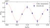 |
Fig. 1. Dependency of the instability growth rate Γ/ωp on the frequency ratio ωp/ωc. Consistent with the theoretical conclusions, the maxima are located at integer values and the minima are between them. |
Providing a closer look at the configurations with ωp/ωc from 10.5 to 11.5 (interval between two subsequent minima), Fig. 2 a shows the temporal evolution of the electrostatic energy scaled to the initial kinetic energy UEx/Ek0. In addition to the configuration with the integer value of ωp/ωc having the highest growth rate, it also exerts the highest saturation energy.
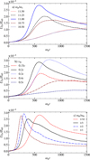 |
Fig. 2. Evolution of the electrostatic energy of the x field component UEx scaled to the initial kinetic energy Ek0. Panel a: evolution of UEx/Ek0, where Ek0 is the total initial kinetic energy for different values of the ratio between plasma and cyclotron frequency ωp/ωc. Panel b: evolution of UEx/Ek0 in relation to the increasing value of the characteristic thermal velocity of the hot plasma component vth. Panel c: evolution of UEx/Ek0 in relation to the increasing value of the ratio between the hot and background plasma density nth/ntb. |
To further build on the foundation of the configuration with the highest saturation energy (ωp/ωc = 11; Table 1, Col. B), five subsequent simulations with an increasing loss-cone characteristic velocity vth were computed in order to investigate whether an increased vth has a positive impact on the instability growth rate and to what extent the saturation value can be increased. The temporal evolution of electrostatic energy scaled to the corresponding initial kinetic energy UEx/Ek0 is shown in Fig. 2b. The configuration with vth = 0.2c shows the highest growth rate Γ relative to the total kinetic energy of the simulation; however, the highest energy ratio UEx/Ek0 is reached in the configuration with vth = 0.3c. Therefore, the highest growth rate is not necessarily accompanied by the highest saturation energy. What is apparent is that the instability grows strongly with vth up to 0.3c. Further increasing the characteristic velocity does not increase both the instability growth rate and saturation value. The decrease of the growth rate at sufficiently high characteristic velocities implies that the efficiency of the instability is low for highly relativistic energies (Verdon & Melrose 2011).
Along with the study of an increasing characteristic velocity vth, we conducted an investigation of an increasing ratio between the hot and background plasma component nth/ntb for four different cases (Table 1, Col. C). Figure 2c shows the temporal evolution of electrostatic energy scaled to the corresponding initial kinetic energy UEx/Ek0 for density ratios nth/ntb = 1/10, 1/3, 1/2, and 1/1. We only considered the x component (with the components of other dimensions averaged) because we primarily focused on effects perpendicular to the magnetic field. Higher density ratios represent the possibility of a more energetic plasma environment, resulting in the instability forming faster and with a higher growth rate Γ; however, the saturation energy is comparable between all studied cases.
3.2. Wave analysis and dispersion of the plasma
The wave dispersion was obtained by analyzing the electric field E in the Fourier space. First and foremost, we compared an electron–proton plasma simulation and an electron–positron one (Table 1, Col. D) under the conditions of low magnetization. The configuration of these referential simulations is identical except for the mass ratio between positive and negative charged particles, where we used m+/m− = 1836 (mass ratio between the proton and electron) for the electron–proton plasma and m+/m− = 1 to represent the electron–positron plasma. The plasma parameters are the frequency ratio ωp/ωc = 5 and the number density ratio nth/ntb = 1/2, 1/10. Even though the electron–positron and the electron–proton plasma have different total plasma frequencies, we assumed that the contribution of the ion plasma frequency to the total plasma frequency is negligible
where me and mi are the electron and ion rest mass, respectively. We scaled the presented quantities for both types of plasma to the total plasma frequency, as the emission occurs close to integer multiples of ωp. In the case of the electron–positron plasma, scaling to ωp is justified since we did not see the separate effects of either the electron or positron plasma frequency in the dispersion. The comparison between the dispersion of the electron–proton and the electron–positron plasma is shown in Fig. 3. In the figure, the dispersion in the x, y, and z components of the electric field E(k⊥, ω) is obtained through the Fourier transform of E(x, t). In the case of the electron–proton plasma, O, X, Z, and Bernstein wave modes were generated, yielding results similar to those obtained in solar plasma simulations (Benáček & Karlický 2019; Ni et al. 2020; Li et al. 2021).
 |
Fig. 3. Dispersion diagrams for electron–proton plasma (left column) and electron–positron plasma (right column) for frequency ratio ωp/ωc = 5 and density ratio between the hot and background plasma nth/ntb = 1/2 (a–b), 1/10 (c–d). The rows show the dispersion in the Ex (longitudinal waves) and Ey (transverse waves). The Bernstein (overlaid red curves), X, Z, X2, and XZ modes are denoted together with plasma frequency ωp (black dotted line). Analytical curves of X2 and XZ modes are overlaid in maroon for electron–positron plasma. |
For our case, the dispersion in Ey is the most important, as it is the transverse field component in which the X and Z modes are generated. The largest difference for the electron–proton plasma is that the plasma does not generate X and Z modes separated in frequency for k⊥ = 0. Instead, an XZ mode is generated. This mode is generated directly at the plasma frequency ωp, as opposed to the X mode being generated above and Z mode below ωp for k⊥ = 0 in the electron–proton plasma. Another difference we noted is the presence of a second extraordinary X2 mode in the dispersion of Ey of the electron–positron plasma, which is in agreement with Iwamoto (1993). Both upper- and lower-branch solutions of the dispersion relation (13) are overlaid onto the electron–positron simulation dispersion in Fig. 3. Apart from these remarks, further differences between both plasma types are essentially indistinguishable, with both plasmas generating Bernstein waves in Ex and identical O mode waves in Ez. The growth rate of the instability is nearly identical between both cases. Furthermore, we computed analytical Bernstein solutions (Benáček & Karlický 2019) and overlaid them onto the interval k < 0. Since k is symmetrical, one can compare the Bernstein modes generated in the simulation with its analytical solutions. However, it is possible to reliably find the analytical solution when the dispersion relation of Eq. (5) holds, in other words, when the loss-cone plasma density is negligible compared to the background plasma density (which is not a good approach for nth/ntb = 1/2).
Based on the first two simulation cycles, we calculated 12 simulations across a range of different density ratios nth/ntb and plasma-to-cyclotron frequency ratios ωp/ωc listed in Table 1(C). The dispersion in the Ex and Ey components of E(x) (perpendicular to the magnetic field) are shown in Figs. 4–6. Each figure shows a dispersion with a fixed frequency ratio ωp/ωc = 11 (Fig. 4), 5 (Fig. 5), and 3 (Fig. 6) for four different configurations with a decreasing density ratio nth/ntb. The dispersion diagrams are overlaid with the frequency ω integrated over the wave number k⊥, noted as the frequency profile F(ω) of the electrostatic Bernstein waves in the longitudinal Ex component and the electromagnetic XZ mode in the transverse Ey component. A separation of these modes from the background is required to integrate the wave modes. The integration was done accurately in the case of the XZ mode, as the curve could be fitted with a hyperbole analytically, and a thin region around the curve of the XZ mode with a frequency half-width 0.2 ωp was selected. In the case of Bernstein waves, however, there is no straightforward analytic solution for the electron–positron plasma due to the high background density compared to the density of the loss-cone plasma. Therefore, a rectangular window encompassing the maxima of the Bernstein wave intensity in the range k⊥c/ωp = −15 to 15, ω = (0 − 1.5)ωp was used, resulting in increased inclusion of noise compared to the integration of the XZ waves. The integrated profiles F(ω) were normalized to the maximum of the top-most case Fmax; therefore, F(ω)/Fmax is equal to one for the top-most case and can be higher or lower for the rest.
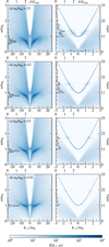 |
Fig. 4. Dispersion diagrams for various values of nth/ntb (rows) with frequency ratio ωp/ωc = 11 for the electron–positron plasma. Left column: Ex. Right column: Ey. Dispersion diagrams are overlaid with an integrated frequency profile scaled to the maximum of the top-most case (nth/ntb = 1). |
Lastly, we present a calculation of the estimated mode energy density for the Bernstein and XZ modes. The estimated energy was obtained through the inverse Fourier transform of the mentioned modes (Bernstein modes in Ex and XZ mode in Ey). The temporal evolution of the mode energy scaled to the initial kinetic energy of the simulations (Table 1(C)) is shown in Fig. 7. Most of the total electrostatic energy is carried by the Bernstein waves (noted as EB), as can be seen by comparing Fig. 7 (bottom left) and Fig. 2b. There is only about a 10% difference between the maxima of the integrated Bernstein waves and the electrostatic energy UEx of the simulation. In other words, the selected Bernstein waves account for approximately 90% of the UEx. In contrast, the electromagnetic energy carried by the XZ modes (noted as EXZ) reaches maxima that are four orders of magnitude lower than those of the Bernstein waves. However, it should be noted that the integration of the Bernstein waves was less accurate than the analytic solution of the XZ mode because the integration includes more field noise.
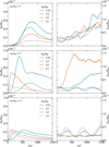 |
Fig. 7. Temporal evolution of energy scaled to the initial kinetic energy of the electrostatic Bernstein waves (left column) and the electromagnetic XZ mode (right column) with frequency ratio ωp/ωc = 3, 5, and 11 (rows) for different values of the hot/background particle density ratio nth/ntb. |
3.3. Velocity distribution function and its evolution
To comprehend and constrain the effects observed in the investigation of how the increasing characteristic thermal velocity vth of the hot plasma component impacts the formation of the instability, we considered the VDF temporal evolution. The existence of a hot population described via the DGH distribution results in a positive gradient in the distribution of the perpendicular velocity u⊥, producing unstable plasma via the DPR effect. The VDF f (v⊥, v∥) (a function of the perpendicular and parallel velocity component) obtained from simulations in Table 1(B) (also Fig. 2b) are shown in Fig. 8. The distributions were computed at the start of the simulations (ωpt = 0) and after 1200 plasma periods (ωpt = 1200). Combining the results from Figs. 2b and 8 shows that a higher growth rate is accompanied by larger shifts in the velocity distribution. For plasma with a lower characteristic velocity (vth ≤ 0.3c), the instability has a higher growth rate due to its positive gradient in f being located at lower u⊥.
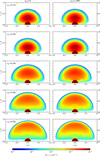 |
Fig. 8. Velocity distribution functions at times ωpt = 0 (left column) and ωpt = 1200 (right column) for an increasing value of the loss-cone characteristic velocity. The distributions have been normalized to the total number of particles N. Combined with Fig. 2b, it is evident that the configurations with higher growth also exert more sizable changes in the velocity distribution function. |
The evolution of the VDF is further visualized in Fig. 9, showing the difference between the initial and evolved VDF f (v⊥, v∥)ωpt = 1200 − f (v⊥, v∥)ωpt = 0 and overlaid with resonance curves corresponding to the solution of Eq. (5) for gyro-harmonic numbers s = 12, 13, 14, and 15, with k∥ set to zero. Including an arbitrary value of k∥ would shift the resonance curves in v∥ space, thus losing the information about the plasma density difference defined by the resonance curves. The scenarios with lower values of vth (up to 0.3c), for which the instability grows exponentially, also show a substantial change between the final and initial state of f (v⊥, v∥). There is a decrease of particles delimited by the resonance curve of s = 12 toward zero perpendicular velocity; however, the particles are shifted to higher velocities periodically between the resonance curves of higher (s > 12) gyro-harmonic numbers.
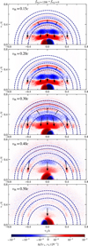 |
Fig. 9. Differences in the velocity distribution functions Δf(v⊥, v∥) between the final (ωpt = 1200) and the initial state (ωpt = 0) for an increasing value of the characteristic thermal velocity vth (rows). The dashed lines represent resonance curves for gyro-harmonic numbers s = 12, 13, 14, 15, with s = 12 being closest to zero velocity. Arrows denote shifts in the VDF contained within the resonance curves. |
4. Discussion and conclusions
The distinct zebra pattern in the Crab pulsar interpulse emission (Hankins & Eilek 2007) could be explained by electron–positron cyclotron maser emission driven via the DPR effect (Zheleznyakov et al. 2016). The cyclotron maser requires a relatively weak magnetic field that can be reached close to current sheets of the magnetic reconnection or in the pulsar wind beyond the light cylinder. Using the modified 3D relativistic PIC code TRISTAN, we computed a few series of simulations surveying the impacts of the plasma-to-cyclotron frequency ratio in the range ωp/ωc = 10 − 12; a characteristic velocity of the hot loss-cone plasma vth = 0.15c − 0.5c; the number density ratio between the background and hot plasma components nth/ntb = 1/1 − 1/10 for frequency ratios ωp/ωc = 3, 5, and 11; and a comparison of the electron–positron with electron–proton plasmas.
When comparing the simulation of the electron–proton plasma with the electron–positron plasma (Fig. 3) for similar plasma parameters and weak magnetization, we observed that distinguishable X (cutoff above ωp) and Z (cutoff below ωp) modes were generated in the electron–proton plasma. In the case of the electron–positron plasma, an XZ mode, which doesn’t have a cutoff at  as the upper branch of the extraordinary mode (Iwamoto 1993) and the lower branch of the extraordinary mode X2 are generated. This XZ mode approaches ωp for k⊥ = 0, with the cutoff frequency having a slight dependence on the density ratio nth/ntb between the hot and background plasma components. A similar dependency of the decreasing cutoff frequency wave mode with an increasing electron temperature was also found in the analytic study by Rafat et al. (2019) for relativistically hot plasmas. Although the X mode moves to higher frequencies and the Z mode moves to lower frequencies, depending on the gyro-frequency in electron–proton plasmas (Li et al. 2021), the XZ mode is generated exclusively near the plasma frequency of the electron–positron plasma. Furthermore, we demonstrated that our first-principle simulation yields plausible results by computing analytical solutions for both the Bernstein and extraordinary waves and comparing them with waves generated in the simulation.
We found that the growth rate of the instability is the highest at integer values of the plasma-to-cyclotron frequency ratio. Our further evaluation of the instability showed that the highest saturation energy, normalized to initial kinetic energy, is reached for loss-cone characteristic velocities vth in the range 0.2−0.3c. The highest saturation energy was obtained in the simulation with vth = 0.3c, while the highest growth rate was obtained for vth = 0.2c. This discrepancy suggests that the highest saturation of the electrostatic energy is not necessarily accompanied by the highest instability growth. Furthermore, increasing the characteristic velocity of the loss-cone component diminishes the instability growth, showing the mechanism is less efficient for relativistically hot plasma where higher energy densities are obtained than for lower characteristic velocities.
We observed a correlation between the growth rate of the instability and the evolution of the VDF f (v⊥, v∥). The highest growth rates are accompanied by the distributions with the most changes over the course of the simulation. While some particles shift to lower perpendicular velocities, others shift to higher velocities. These changes in the VDF are encompassed by DPR resonance curves.
Even though the instability growth rate peaks are found at integer values of the frequency ratio ωp/ωc, this does not necessarily imply that the strongest intensity of the electrostatic and electromagnetic waves is located at frequencies of the cyclotron harmonics. The intensity maxima of the electromagnetic waves, determined in the dispersion of the electric field components (Figs. 4–6), are located mainly at frequencies between the gyro-harmonics. Furthermore, these maxima of wave intensity in the ω − k⊥ domain are contained within the frequency range ω = 1 − 2 ωp.
The particle number density ratio shifts in the phase space (see Fig. 9) with the resonance curves of the gyro-harmonics slightly above the plasma frequency, and their intensity gradually decreases when increasing the gyro-harmonic number s, effectively constraining the emission within the resulting frequency range. Thus, the electron–positron maser instability driven via the DPR effect could be the mechanism responsible for the generation of the narrowband emission observed in the dynamic spectra of the Crab pulsar (Hankins & Eilek 2007).
The effects of DPR in the direction parallel to the magnetic field have not yet been studied in 2D and 3D electron–positron PIC simulations, to the best of our knowledge. If the parallel waves are resolved in 2D and 3D, the wave number k∥ in the resonance condition of Eq. (5) is nonzero, and more resonating particles may contribute to the electrostatic wave generation. That leads to a different pattern in the velocity distribution temporal changes. The currently detected resonance changes in Fig. 9 do not appear as ellipses, but a particle distribution changes its shape relatively smoothly. The smooth change was shown, for example, by Benáček & Karlický (2018, Fig. 3) and Ni et al. (2020, Fig. 1) for electron–ion plasma, and it occurs as the positions of resonance ellipses shift with k∥.
The most intensive electrostatic waves are generated in the mostly perpendicular direction for electron–ion plasma (Li et al. 2021). For oblique waves, the electrostatic wave intensity decreases. If we expect a similar behavior for electron–positron plasma, our results on the intensity could be understood as the upper limit of the electrostatic waves that are produced perpendicular to the magnetic field. However, in more dimensions, the electromagnetic waves could be easier to generate by wave coalescence because various wave numbers with nonzero k∥ can contribute simultaneously and enhance our estimated power. In addition, the produced electromagnetic waves can have oblique directions not covered by 1D simulations. Nonetheless, the resonances at gyro-harmonics appear and may still be considered responsible for varying saturation energies with changing ωp/ωc ratio in more dimensions (Li et al. 2021).
4.1. Constraints on radio emission region
With the currently considered model of the zebra emission, we can constrain the density ratio in the emission region. Because the frequency distances between observed zebra stripes are not constant, the individual stripes are generated in various plasma regions as the ratio between the plasma density and cyclotron frequency changes. This implies that each emission region emits at only one specific frequency, and the observed zebra pattern is produced as a compilation of several emission regions. Therefore, the maser mechanism also has to emit at one specific frequency. Assuming the XZ mode emission, the density ratio nth/ntb ≲ 1/10 is required to fulfill the condition. On the other hand, if a zebra pattern with an equal frequency distance between stripes is observed, the emission can be produced by one plasma region with a high density ratio nth/ntb ≳ 1/1. Moreover, the density ratio increases with the number of detected stripes.
The emission generation is a two-step process. First, the kinetic instability excites arbitrary electrostatic wave modes. The electromagnetic waves are then generated through the coalescence of the electrostatic modes. In the solar plasma, Z mode, and Bernstein (UH) mode, coalescence accounts for the cyclotron maser emission (Ni et al. 2020). In the electron–positron plasma, a coalescence of two Bernstein modes (Kuznetsov 2005) into the XZ mode may account for the observed quasi-harmonic emission of the pulsar radio interpulse. This can be seen in Fig. 5b, where the highest peak of the XZ mode is at the double frequency of the highest peak of the Bernstein modes. This indicates that the radio emission is produced by a coalescence of two Bernstein modes with the same frequency and opposite wave numbers. The coalescence process, however, is ineffective, as the XZ mode reaches energies approximately four orders of magnitude lower than those of the Bernstein modes (Fig. 7). Moreover, since our PIC simulation is grid based, any coalescence-based process is inherently less effective due to a limited set of wave vectors k included in the simulation. Because the emission region generates the emission at one frequency, other zebra stripes need to be generated at different locations, which explains the nonconstant spacing between zebra stripes.
4.2. Estimation of flux density
To present an estimate of the generated flux density of the electromagnetic emission, we based our calculation on the simulation with the strongest XZ mode (ωp/ωc = 5, nth/ntb = 1/2). We estimated the radiative flux under the following assumptions: (1) the energy of the XZ mode is scaled to the total kinetic energy of the simulation; (2) the area of the source is 100 km2; (3) the distance to the source is 1 kpc (distance of the Crab pulsar is approximately 2 kpc); and (4) the radiative transfer effects are neglected. The kinetic energy of a particle is given by
Considering the upper limit of the particle number density (Zheleznyakov et al. 2016) n = 1.2 × 1011 cm−3, the estimated total kinetic energy density is
The highest energy of the XZ mode obtained from the simulations is ≈1.5 × 10⁻⁷ Ek. Under the above-mentioned assumptions, we obtained a radiative flux P ∼ 1 mJy. Taking into account the emission source velocity (β = 0.82), the received flux is P ∼ 30 mJy. This value is considerably lower than the observed radiative flux density (Hankins & Eilek 2007) by approximately four to five orders of magnitude; however, one should bear in mind that the domain size of the presented simulations was small (≈350 cm3) and effectively 1D. On the other hand, 2D or even 3D simulations could simulate the effects of an arbitrary propagation angle instead of limiting us to the perpendicular propagation to the magnetic field. Furthermore, due to the grid-based nature of our simulation, any coalescence process is less effective. A relatively low particle number density can be responsible for the widening of the frequency peaks due to the effects of the numerical noise.
The Doppler effect could increase the power of the emitted waves if the emission source moves toward the observer with a higher velocity than assumed above. The Lorentz factor for such a Doppler boost can be obtained on the order of γ ∼ 102 − 104 in the pulsar wind (Lin et al. 2023). That could lead to an increase of the emitted power by a factor of ∝γ3 for γ ≫ 1 (Rybicki & Lightman 2004, Chap. 4.8). This way, for γ ∼ 103 we can obtain the emission power of ∼106 Jy. However, we must note that the Doppler effect does not only increase the power, but it also increases the wave frequency. Hence, for the same observed frequency, the Doppler frequency shift would require wave emission at frequencies much lower than the plasma frequency, much lower plasma frequencies, or kinetic and “XZ” mode energy densities higher than estimated for our case.
We conclude that the detected emission power from our PIC simulations is too low to explain the observed intensities of the zebra pattern. To obtain the observed intensities, the area of the emission region or the conversion efficiency from particles to electromagnetic waves is required to be about five orders of magnitude higher. Therefore, future considerations of the electron–cyclotron maser instability should include two-dimensional analysis of the (k⊥, k∥) space in order to determine whether the radiation is exclusively generated in a wide or narrow angle, how the radiative power depends on the emission angle, and what the contribution by the relativistic beaming effect is. Furthermore, a larger domain size would allow for a much less limited set of k vectors, which might increase the efficiency of the coalescence process.
Acknowledgments
M.L. acknowledges the GACR-LA grant no. GF23-04053L for financial support. J.B. acknowledges support from the German Science Foundation (DFG) projects BU 777-17-1 and BE 7886/2-1. M.K. acknowledges support from the GACR grant no. 21-16508J. This work was supported by the Ministry of Education, Youth and Sports of the Czech Republic through the e-INFRA CZ (ID:90140). The authors gratefully acknowledge the Gauss Centre for Supercomputing e.V. (https://www.gauss-centre.eu) for funding this project by providing computing time on the GCS Supercomputer SuperMUC at Leibniz Supercomputing Centre (www.lrz.de).
References
- Babul, A.-N., & Sironi, L. 2020, MNRAS, 499, 2884 [NASA ADS] [CrossRef] [Google Scholar]
- Beloborodov, A. M. 2008, ApJ, 683, L41 [NASA ADS] [CrossRef] [Google Scholar]
- Benáček, J., & Karlický, M. 2018, A&A, 611, A60 [NASA ADS] [CrossRef] [EDP Sciences] [Google Scholar]
- Benáček, J., & Karlický, M. 2019, ApJ, 881, 21 [CrossRef] [Google Scholar]
- Benáček, J., Karlický, M., & Yasnov, L. V. 2017, A&A, 598, A106 [NASA ADS] [CrossRef] [EDP Sciences] [Google Scholar]
- Benáček, J., Muñoz, P. A., & Büchner, J. 2021a, ApJ, 923, 99 [CrossRef] [Google Scholar]
- Benáček, J., Muñoz, P. A., Manthei, A. C., & Büchner, J. 2021b, ApJ, 915, 127 [CrossRef] [Google Scholar]
- Benáček, J., Muñoz, P. A., Büchner, J., & Jessner, A. 2023, A&A, 675, A42 [NASA ADS] [CrossRef] [EDP Sciences] [Google Scholar]
- Bernstein, I. B. 1958, Phys. Rev., 109, 10 [NASA ADS] [CrossRef] [Google Scholar]
- Bilbao, P. J., & Silva, L. O. 2023, Phys. Rev. Lett., 130, 165101 [CrossRef] [Google Scholar]
- Boris, J. P., Dawson, J. M., Orens, J. H., & Roberts, K. V. 1970, Phys. Rev. Lett., 25, 706 [NASA ADS] [CrossRef] [Google Scholar]
- Buneman, O. 1993, in Computer Space Plasma Physics: Simulation Techniques and Software, eds. H. Matsumoto, & Y. Omura (Terra Scientific Publishing Company), 67 [Google Scholar]
- Buschauer, R., & Benford, G. 1977, MNRAS, 179, 99 [Google Scholar]
- Cerutti, B., Philippov, A. A., & Dubus, G. 2020, A&A, 642, A204 [NASA ADS] [CrossRef] [EDP Sciences] [Google Scholar]
- Chernov, G. P., Yan, Y. H., Fu, Q. J., & Tan, C. M. 2005, A&A, 437, 1047 [NASA ADS] [CrossRef] [EDP Sciences] [Google Scholar]
- Dory, R. A., Guest, G. E., & Harris, E. G. 1965, Phys. Rev. Lett., 14, 131 [CrossRef] [Google Scholar]
- Eilek, J. A., & Hankins, T. H. 2016, J. Plasma Phys., 82, 635820302 [Google Scholar]
- Elgarøy, Ø. 1961, Astrophys. Nor., 7, 123 [Google Scholar]
- Fung, P. K., & Kuijpers, J. 2004, A&A, 422, 817 [NASA ADS] [CrossRef] [EDP Sciences] [Google Scholar]
- Gil, J., Lyubarsky, Y., & Melikidze, G. I. 2004, ApJ, 600, 872 [NASA ADS] [CrossRef] [Google Scholar]
- Hankins, T. H., & Eilek, J. A. 2007, ApJ, 670, 693 [Google Scholar]
- Hankins, T. H., & Rankin, J. M. 2010, AJ, 139, 168 [NASA ADS] [CrossRef] [Google Scholar]
- Hankins, T. H., Jones, G., & Eilek, J. A. 2015, ApJ, 802, 130 [NASA ADS] [CrossRef] [Google Scholar]
- Hankins, T. H., Eilek, J. A., & Jones, G. 2016, ApJ, 833, 47 [NASA ADS] [CrossRef] [Google Scholar]
- Iwamoto, N. 1993, Phys. Rev. E, 47, 604 [NASA ADS] [CrossRef] [Google Scholar]
- Kazbegi, A. Z., Machabeli, G. Z., & Melikidze, G. I. 1991, MNRAS, 253, 377 [CrossRef] [Google Scholar]
- Kuijpers, J. 1975, Sol. Phys., 44, 173 [NASA ADS] [CrossRef] [Google Scholar]
- Kuznetsov, A. A. 2005, A&A, 438, 341 [NASA ADS] [CrossRef] [EDP Sciences] [Google Scholar]
- Li, C., Chen, Y., Ni, S., et al. 2021, ApJ, 909, L5 [NASA ADS] [CrossRef] [Google Scholar]
- Lin, R., van Kerkwijk, M. H., Main, R., et al. 2023, ApJ, 945, 115 [NASA ADS] [CrossRef] [Google Scholar]
- Litvinenko, G. V., Shaposhnikov, V. E., Konovalenko, A. A., et al. 2016, Icarus, 272, 80 [NASA ADS] [CrossRef] [Google Scholar]
- Lyubarsky, Y. 2009, ApJ, 696, 320 [NASA ADS] [CrossRef] [Google Scholar]
- Lyutikov, M. 2021, ApJ, 922, 166 [CrossRef] [Google Scholar]
- Lyutikov, M., Blandford, R. D., & Machabeli, G. 1999, MNRAS, 305, 338 [NASA ADS] [CrossRef] [Google Scholar]
- Manthei, A. C., Benáček, J., Muñoz, P. A., & Büchner, J. 2021, A&A, 649, A145 [NASA ADS] [CrossRef] [EDP Sciences] [Google Scholar]
- Matsumoto, H., & Omura, Y. 1993, Computer Space Plasma Physics: Simulation Techniques and Software (Terra Scientific Pub. Co.) [Google Scholar]
- Melikidze, G. I., Gil, J. A., & Pataraya, A. D. 2000, ApJ, 544, 1081 [NASA ADS] [CrossRef] [Google Scholar]
- Melrose, D. B., & Gedalin, M. E. 1999, ApJ, 521, 351 [Google Scholar]
- Melrose, D. B., Rafat, M. Z., & Mastrano, A. 2021, MNRAS, 500, 4530 [Google Scholar]
- Mitra, D. 2017, JApA, 38, 52 [NASA ADS] [Google Scholar]
- Ni, S., Chen, Y., Li, C., et al. 2020, ApJ, 891, L25 [NASA ADS] [CrossRef] [Google Scholar]
- Ning, H., Chen, Y., Ni, S., et al. 2021, ApJ, 920, L40 [NASA ADS] [CrossRef] [Google Scholar]
- Pearlstein, L. D., Rosenbluth, M. N., & Chang, D. B. 1966, Phys. Fluids, 9, 953 [NASA ADS] [CrossRef] [Google Scholar]
- Petrova, S. A. 2009, MNRAS, 395, 1723 [Google Scholar]
- Philippov, A., Timokhin, A., & Spitkovsky, A. 2020, Phys. Rev. Lett., 124, 245101 [Google Scholar]
- Rafat, M. Z., Melrose, D. B., & Mastrano, A. 2019, J. Plasma Phys., 85, 905850305 [Google Scholar]
- Ruderman, M. A., & Sutherland, P. G. 1975, ApJ, 196, 51 [Google Scholar]
- Rybicki, G. B., & Lightman, A. P. 2004, Radiative Processes in Astrophysics (Weinheim: Wiley) [Google Scholar]
- Schneider, J. 1959, Phys. Rev. Lett., 2, 504 [NASA ADS] [CrossRef] [Google Scholar]
- Sturrock, P. A. 1971, ApJ, 164, 529 [Google Scholar]
- Timokhin, A. N., & Arons, J. 2013, MNRAS, 429, 20 [NASA ADS] [CrossRef] [Google Scholar]
- Twiss, R. Q. 1958, Aust. J. Phys., 11, 564 [NASA ADS] [CrossRef] [Google Scholar]
- Ursov, V. N., & Usov, V. V. 1988, Ap&SS, 140, 325 [NASA ADS] [CrossRef] [Google Scholar]
- Usov, V. V. 1987, ApJ, 320, 333 [Google Scholar]
- Verdon, M. W., & Melrose, D. B. 2011, Phys. Rev. E, 83, 056407 [NASA ADS] [CrossRef] [Google Scholar]
- Villasenor, J., & Buneman, O. 1992, Comput. Phys. Commun., 69, 306 [NASA ADS] [CrossRef] [Google Scholar]
- Weatherall, J. C. 1994, ApJ, 428, 261 [Google Scholar]
- Winglee, R. M., & Dulk, G. A. 1986, ApJ, 307, 808 [Google Scholar]
- Yao, X., Muñoz, P. A., Büchner, J., et al. 2022, ApJ, 933, 219 [NASA ADS] [CrossRef] [Google Scholar]
- Yasnov, L. V., Benáček, J., & Karlický, M. 2017, Sol. Phys., 292, 163 [NASA ADS] [CrossRef] [Google Scholar]
- Yee, K. 1966, IEEE Trans. Antennas Propag., 14, 302 [Google Scholar]
- Zhdankin, V., Kunz, M. W., & Uzdensky, D. A. 2023, ApJ, 944, 24 [NASA ADS] [CrossRef] [Google Scholar]
- Zheleznyakov, V. V. 1971, Ap&SS, 13, 87 [NASA ADS] [CrossRef] [Google Scholar]
- Zheleznyakov, V. V., & Shaposhnikov, V. E. 2020, MNRAS, 495, 3715 [NASA ADS] [CrossRef] [Google Scholar]
- Zheleznyakov, V. V., & Zlotnik, E. Y. 1975a, Sol. Phys., 43, 431 [NASA ADS] [CrossRef] [Google Scholar]
- Zheleznyakov, V. V., & Zlotnik, E. Y. 1975b, Sol. Phys., 44, 447 [NASA ADS] [CrossRef] [Google Scholar]
- Zheleznyakov, V. V., & Zlotnik, E. Y. 1975c, Sol. Phys., 44, 461 [Google Scholar]
- Zheleznyakov, V. V., Zaitsev, V. V., & Zlotnik, E. Y. 2012, Astron. Lett., 38, 589 [NASA ADS] [CrossRef] [Google Scholar]
- Zheleznyakov, V., Zlotnik, E., Zaitsev, V., & Shaposhnikov, V. 2016, Uspekhi Fizicheskih Nauk, 186, 037813 [Google Scholar]
- Zlotnik, E. Y., Zaitsev, V. V., Aurass, H., Mann, G., & Hofmann, A. 2003, A&A, 410, 1011 [NASA ADS] [CrossRef] [EDP Sciences] [Google Scholar]
All Tables
All Figures
|
Fig. 1. Dependency of the instability growth rate Γ/ωp on the frequency ratio ωp/ωc. Consistent with the theoretical conclusions, the maxima are located at integer values and the minima are between them. |
| In the text | |
|
Fig. 2. Evolution of the electrostatic energy of the x field component UEx scaled to the initial kinetic energy Ek0. Panel a: evolution of UEx/Ek0, where Ek0 is the total initial kinetic energy for different values of the ratio between plasma and cyclotron frequency ωp/ωc. Panel b: evolution of UEx/Ek0 in relation to the increasing value of the characteristic thermal velocity of the hot plasma component vth. Panel c: evolution of UEx/Ek0 in relation to the increasing value of the ratio between the hot and background plasma density nth/ntb. |
| In the text | |
|
Fig. 3. Dispersion diagrams for electron–proton plasma (left column) and electron–positron plasma (right column) for frequency ratio ωp/ωc = 5 and density ratio between the hot and background plasma nth/ntb = 1/2 (a–b), 1/10 (c–d). The rows show the dispersion in the Ex (longitudinal waves) and Ey (transverse waves). The Bernstein (overlaid red curves), X, Z, X2, and XZ modes are denoted together with plasma frequency ωp (black dotted line). Analytical curves of X2 and XZ modes are overlaid in maroon for electron–positron plasma. |
| In the text | |
|
Fig. 4. Dispersion diagrams for various values of nth/ntb (rows) with frequency ratio ωp/ωc = 11 for the electron–positron plasma. Left column: Ex. Right column: Ey. Dispersion diagrams are overlaid with an integrated frequency profile scaled to the maximum of the top-most case (nth/ntb = 1). |
| In the text | |
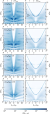 |
Fig. 5. Same as Fig. 4 but for ωp/ωc = 5. |
| In the text | |
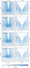 |
Fig. 6. Same as Fig. 4 but for ωp/ωc = 3. |
| In the text | |
|
Fig. 7. Temporal evolution of energy scaled to the initial kinetic energy of the electrostatic Bernstein waves (left column) and the electromagnetic XZ mode (right column) with frequency ratio ωp/ωc = 3, 5, and 11 (rows) for different values of the hot/background particle density ratio nth/ntb. |
| In the text | |
|
Fig. 8. Velocity distribution functions at times ωpt = 0 (left column) and ωpt = 1200 (right column) for an increasing value of the loss-cone characteristic velocity. The distributions have been normalized to the total number of particles N. Combined with Fig. 2b, it is evident that the configurations with higher growth also exert more sizable changes in the velocity distribution function. |
| In the text | |
|
Fig. 9. Differences in the velocity distribution functions Δf(v⊥, v∥) between the final (ωpt = 1200) and the initial state (ωpt = 0) for an increasing value of the characteristic thermal velocity vth (rows). The dashed lines represent resonance curves for gyro-harmonic numbers s = 12, 13, 14, 15, with s = 12 being closest to zero velocity. Arrows denote shifts in the VDF contained within the resonance curves. |
| In the text | |
Current usage metrics show cumulative count of Article Views (full-text article views including HTML views, PDF and ePub downloads, according to the available data) and Abstracts Views on Vision4Press platform.
Data correspond to usage on the plateform after 2015. The current usage metrics is available 48-96 hours after online publication and is updated daily on week days.
Initial download of the metrics may take a while.