| Issue |
A&A
Volume 627, July 2019
|
|
|---|---|---|
| Article Number | A30 | |
| Number of page(s) | 11 | |
| Section | Numerical methods and codes | |
| DOI | https://doi.org/10.1051/0004-6361/201935161 | |
| Published online | 27 June 2019 | |
ExPRES: an Exoplanetary and Planetary Radio Emissions Simulator
1
Institut de Recherche en Astrophysique et Planétologie (IRAP), Université de Toulouse, CNRS CNES, Université Paul Sabatier, Toulouse, France
e-mail: This email address is being protected from spambots. You need JavaScript enabled to view it.
2
LESIA, Observatoire de Paris, PSL Research University, CNRS, Sorbonne Universités, UPMC Univ. Paris 06, Univ. Paris Diderot, Sorbonne Paris Cité, Meudon, France
3
USN, Observatoire de Paris, CNRS, PSL, UO/OSUC, Nançay, France
4
ONERA-The French Aerospace Lab, 31055 Toulouse, France
5
DIO, Observatoire de Paris, PSL Research University, CNRS, Paris, France
Received:
28
January
2019
Accepted:
20
May
2019
Abstract
Context. Earth and outer planets are known to produce intense non-thermal radio emissions through a mechanism known as cyclotron maser instability (CMI), requiring the presence of accelerated electrons generally arising from magnetospheric current systems. In return, radio emissions are a good probe of these current systems and acceleration processes. The CMI generates highly anisotropic emissions and leads to important visibility effects, which have to be taken into account when interpreting the data. Several studies have shown that modelling the radio source anisotropic beaming pattern can reveal a wealth of physical information about the planetary or exoplanetary magnetospheres that produce these emissions.
Aims. We present a numerical tool, called ExPRES (Exoplanetary and Planetary Radio Emission Simulator), which is able to reproduce the occurrence in a time-frequency plane of R−X CMI-generated radio emissions from planetary magnetospheres, exoplanets, or star–planet interacting systems. Special attention is given to the computation of the radio emission beaming at and near its source.
Methods. We explain what physical information about the system can be drawn from such radio observations, and how it is obtained. This information may include the location and dynamics of the radio sources, the type of current system leading to electron acceleration and their energy, and, for exoplanetary systems, the orbital period of the emitting body and the strength, rotation period, tilt, and the offset of the planetary magnetic field. Most of these parameters can only be remotely measured via radio observations.
Results. The ExPRES code provides the proper framework of analysis and interpretation for past, current, and future observations of planetary radio emissions, as well as for future detection of radio emissions from exoplanetary systems (or magnetic, white dwarf–planet or white dwarf–brown dwarf systems). Our methodology can be easily adapted to simulate specific observations once effective detection is achieved.
Key words: planets and satellites: aurorae / radio continuum: planetary systems / planet-star interactions
© C. K. Louis et al. 2019
 Open Access article, published by EDP Sciences, under the terms of the Creative Commons Attribution License (http://creativecommons.org/licenses/by/4.0), which permits unrestricted use, distribution, and reproduction in any medium, provided the original work is properly cited.
1. Introduction
Earth and outer planets, which possess an internal magnetic field and an atmosphere, are known to emit low-frequency radio emissions in wavelength domains extending from kilometer (below ∼100 kHz) up to decameter (a few tens of MHz – in the case of Jupiter only). The frequency domain corresponds to the electron cyclotron frequencies (fce) close to the planet, revealing that the emission process is related to the electron gyration along the magnetic field lines of the planet. Theoretical work and in situ observations of the terrestrial, kronian, and jovian radio sources allow the physical process at the origin of the radio emissions to be elucidated, namely the cyclotron-maser instability (CMI). This instability occurs when an elliptically polarized wave resonates with the gyration motion of accelerated electrons (see Wu 1985; Louarn 1992; Zarka 1998; Treumann 2006; Louarn et al. 2017; Lamy et al. 2018). The CMI mainly amplifies the wave on the extraordinary R−X mode which can escape the source and propagate in free space as a radio wave.
The interest for planetary low-frequency radio emissions is linked to their relation with accelerated electrons. Those electrons are also responsible for auroral emissions on top of the atmosphere of the planet (over a broad spectral domain extending from infrared to X-rays) and reveal the presence of field-aligned currents coupling the magnetosphere to the ionosphere. Contrary to the other auroral emissions, radio emissions are not emitted on top of the atmosphere, but along a larger altitude range extending from the top of the ionosphere up to a few planet radii (see review by Zarka 1998). The emission frequency is close to fce in the source, itself proportional to the local magnetic field strength which decreases with increasing altitude. Therefore, the radio source altitude can be deduced from the frequency at which it emits. This property can be used to probe large altitude ranges above the aurorae and to reveal, for example, the presence of acceleration regions (Pottelette & Pickett 2007; Hess et al. 2007a, 2010a).
The CMI is very sensitive to the plasma characteristics in the source, such as the density and temperature of the different electron populations, and the shape of the electron velocity distribution (Pritchett 1984; Louarn & Le Quéau 1996a). These parameters not only condition and affect the amplification and the propagation of the wave, but they also have a huge impact on the beaming pattern of the emission (see Sect. 3.3). Typical CMI emissions are radiated over a few degrees (Kaiser et al. 2000; Zarka 2004; Panchenko & Rucker 2016) of a given angle relative to the magnetic field. By symmetry around the magnetic field direction, the emission pattern is a thin hollow cone. This strong anisotropy of the radio emission beaming has two consequences regarding the observations of planetary auroral radio emission: (1) the observations have to be detrended from the source visibility effects before being interpreted – no detection of the emission does not mean that no emission is produced –, and (2) as the beaming pattern strongly depends on the plasma characteristics close to the source, the visibility of the emissions carries information about the plasma parameters at the source.
Visibility effects are responsible for the ubiquitous arc shapes of the radio emission patterns in the time-frequency plane, as illustrated by the examples displayed in Figs. 1a and b that show typical emissions from Jupiter (Queinnec & Zarka 1998) and from Saturn, respectively (including arcs generated by hot-spots in sub-corotation in the magnetosphere of Saturn, Lamy et al. 2008, 2013). The arc shape is a direct consequence of the hollow cone beaming pattern of the source, as shown in Figs. 1c–e in the simple case of a dipolar-axisymetric magnetic field. The radio emission from a radiating field line is received once when the source is on the western side of the observer’s meridian (i.e. before the meridian relative to the sense of planetary rotation) and that one side of the cone is directed toward the observer. It is observed again when the field line is on the eastern side of the meridian and the other side of the cone is directed toward the observer. As a result, for a fixed observer and a field line moving in the sense of rotation, radio emission at a given frequency can be observed twice, once, or not at all depending on the geometry of the beaming pattern.
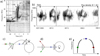 |
Fig. 1. Panels a and b: examples of time-frequency radio arcs. Panel a: radio arcs emitted by the Io-Jupiter interaction (Queinnec & Zarka 1998), observed by Wind (0–15 MHz) and the Nançay Decameter Array (15–40 MHz). Panel b: radio arcs at Saturn, observed by Cassini, related to a sub-corotating hot spot in the magnetosphere of Saturn (Lamy et al. 2008). Panels c and d: side and polar views of the emission geometry, with two sources located along the same magnetic field line but at different altitudes. Arrows show the direction of propagation of the radio waves which can be seen by an observer located in the equatorial plane far from the planet. Panels e: dynamic spectrum of the emissions which would correspond to the geometry of panels c and d. |
To interpret observations of planetary auroral radio emission, it is therefore necessary to take into account its beaming pattern and the source position to infer the effect of the visibility of the source. For some case studies, for example of specific radio arcs, the source location and beaming pattern can be deduced from the observed arc shape, assuming a constant beaming angle along the field lines (Genova & Aubier 1985; Lecacheux et al. 1998), or a beaming angle varying with the frequency (Queinnec & Zarka 1998; Hess et al. 2008, 2014; Ray & Hess 2008; Imai et al. 2008, 2011). Others used a source location provided by an independent method to retrieve the beaming angle, such as the radio goniopolarimetry/direction-finding method, a spinning spacecraft (Kurth et al. 1975; Panchenko 2003; Ladreiter et al. 1994; Imai et al. 2017), a non-spinning spacecraft (Cecconi et al. 2009; Lamy et al. 2011), or the very long baseline interferometry (VLBI) technique (Mutel et al. 2003) using multiple satellites. Deriving physical source parameters directly from observations can be qualified as “inverse modelling”. It allows source and emission parameters that are consistent with a given observation of a radio arc to be inferred, but it does not prove that only the observed arc should indeed be visible at the time of observation, that is it does not entirely de-trend the observation from the beaming effect. Moreover, inverse modelling often implies that both the position and the beaming pattern from a single observation are determined, however these two parameters are strongly coupled, leading to degeneracy of the solution (Hess et al. 2010a).
For a more global interpretation of radio dynamic spectra, a “forward modelling” approach may be better: this consists of assuming source and emission parameters for computing a predicted dynamic spectrum, which is then compared to the observations Louis et al. (2017a,b). A match between the predicted and observed dynamic spectra is strong proof of the effectiveness of the model in reproducing the true source parameters and emission process. Of course, good matches may be obtained for non-unique sets of parameters. Nevertheless, modelling of various observations corresponding to different viewing geometries is expected to remove this degeneracy and allow the source conditions to be better constrained.
Implementing this forward modelling approach is the purpose of the numerical code described in the present paper, the Exoplanetary and Planetary Radio Emission Simulator (ExPRES). This code uses as inputs the geometry of the observation (observer and celestial body positions, source location, and magnetic field topology), the plasma parameters in the sources and their vicinity (density and temperature), as well as the characteristics of the wave-particle interaction generating the radio emissions constrained by the CMI theory. From these inputs, the code computes the beaming pattern of the radio sources, compares the direction of emissions to the direction of the observer, and generates time-frequency visibility maps that can be directly compared to observed dynamic spectra (Sect. 2).
In the following, we summarise the physics of planetary auroral radio emissions and how it is taken into account in ExPRES, starting with the magnetospheric interactions powering the emissions and their impact on the CMI (Sect. 3). We then more specifically discuss the radio emission beaming (Sect. 4). We show that the different cases of auroral radio emission observed in our solar system can be described using a small number of parameters that define both the location of the sources and their beaming pattern. Finally we describe the output parameters of the code, show some simulation examples, and list simulation results already obtained with ExPRES. We conclude by mentioning some limitations of, and perspectives for, the code (Sect. 5).
2. ExPRES modelling
The computation of a synthetic dynamic spectrum with ExPRES mostly relies on the observation geometry. One example is shown in Fig. 2, which sketches the geometry of the observation of emissions triggered by the Io-Jupiter interaction. For a given source–observer geometry (relative positions of the source and the observer at a given time and for a given emission frequency), magnetic field orientation in the source (depending on a magnetic field model), and beaming pattern (depending on electron densities and energies at the source, as discussed in Sect. 4), the code compares the direction of beamed R−X mode waves with the source-to-observer direction. If the angle between these directions is smaller than the beam width, defined by the user, the corresponding time-frequency pixel in the synthetic dynamic spectrum is incremented by one, otherwise it is not. By repeating this computation at all time-frequency steps of interest, for all elementary point sources constituting the user-defined radio source, a visibility map is generated in the time-frequency plane. ExPRES counts by default a standard intensity value of one (unit-less) for each radio source. More physical intensities can nonetheless be used to achieve realistic simulations (see example in Lamy et al. 2013).
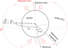 |
Fig. 2. Examples of the geometry involved in the modelling of the Io-controlled emissions of Jupiter. The emission depends on the relative position of Io, Jupiter, and the observer, in particular on the jovigraphic longitude of the observer (λCML, i.e. the central meridian longitude) and that of the active field line which can differ from that of Io (λIo) by a lead angle (δλ). |
The set of parameters that the user needs to feed ExPRES with in order to perform a simulation run is as follows.
– The definition of the celestial bodies involved in the simulation (star, planet, satellite), with their respective positions at each time step (pre-computed or deduced from initial positions and orbital parameters), their rotation or revolution period, and their size and mass. These parameters permit the user to precisely define the geometry of the celestial bodies involved in the simulation.
– The position of the observer relative to the reference body at each time step.
– The magnetic field and density models attached to the bodies of interest (e.g. planet, Sun, planet-star or planet-satellite system). The magnetic field model may be dipolar or of higher order, and the magnetic field lines need to be pre-computed. The density profiles may be that of an ionosphere (exponential decrease with distance from the centre of the body), a stellar corona (decrease in inverse square of the distance from the centre), a plasma disk (exponential decreases from both the equatorial plane and the centre of the body, with different scale heights), or a plasma torus (exponential decrease from the centre of a torus of given radius around the body). These parameters enter in the definition of the characteristics of the radio emission, in particular its beaming angle (see Sect. 4).
– The spatial distribution of sources, that is the position of the magnetic field lines carrying the current (from their footprint longitude and latitude, their equatorial longitude and distance, or their attachment to a satellite) and the frequency range over which the simulation is to be performed.
– The information used to calculate the opening θ of the beaming cone (i.e. the distribution function and the energy of the resonating electrons involved in the radio emission; see Sect. 3) and the thickness Δθ of the beaming conical sheet.
While the source–observer geometry and the magnetic field, plasma density, and energy models at the sources are user-defined in ExPRES, the beaming angle θ is self-consistently computed by the code from beaming models described in Sect. 4 that are based on the CMI theory described in Sect. 3.3. Nevertheless, test simulations may be performed with a predefined beaming angle profile versus frequency (e.g. θ(f) constant or linearly varying with frequency).
ExPRES simulations can be adjusted to observations by varying one or several input parameters (e.g. the electrons energy), and the quality (and possibly uniqueness) of the obtained fit permits to derive the value of the corresponding parameter(s) (Hess et al. 2010a).
3. Radiosource locations and characteristics
3.1. Magnetospheric currents
The auroral radio emissions simulated by ExPRES are deeply related to the dynamics of the magnetosphere of magnetized planets. The magnetosphere is the region where the plasma motion is dominated by the magnetic field of the planet. In first approximation, the plasma and the magnetic field are frozen-in. However, the magnetosphere undergoes constraints – both external (solar wind flow) and internal (e.g. centrifugal forces, satellite outgassing) – that force the plasma motion relative to the magnetic field. This motion creates an electric field with an associated current, which in turn induces a magnetic field that distorts the magnetic field lines to try to keep them frozen in the plasma. Although this is a crude and over-simplified way to summarise magnetospheric physics, it is as a first approximation sufficient to understand the physics involved in the present paper.
The electric currents follow the magnetic field lines – because the conductivity parallel to the magnetic field is far larger than that perpendicular to it – and close in or above the ionosphere of the planet. At some point along the magnetic field line, usually within ∼1 planetary radius above the ionosphere, the increase in magnetic field strength generates a resistance to the current and thus an electric field parallel to the magnetic field. Electrons accelerated by these electric fields precipitate in the atmosphere of the planet and generate aurorae. Outside the accelerating region, these electrons move adiabatically, at least in first approximation, meaning that their parallel velocity v∥ decreases with the magnetic field strength B:
 (1)
(1)
with μ being the magnetic moment of the electrons. If v∥ goes to zero before the electrons reach the ionosphere (where they get lost by collisions and power infrared to X-ray aurorae), they are reflected and can contribute to the radio emission generation via the CMI.
The three main magnetospheric interactions that lead to electron acceleration are as follows.
– The flow of the solar wind, which deforms the magnetosphere to give it a comet-like shape. This leads to the convection of magnetic field lines from the front to the tail of the magnetosphere, with the generation of one or two convection cells, or to viscous interaction along the magnetospheric border. Along with convection cells, an auroral oval fixed in local time (although modulated by the planet rotation) is formed at the footprints of field lines returning toward the front of the magnetosphere (Dungey 1961). Viscous interactions rather lead to less structured and less stationary aurorae, with a strong local time asymmetry (Axford & Hines 1961; Delamere & Bagenal 2010).
– The centrifugal motion of plasma generated inside the magnetosphere. As it moves outward, the conservation of the momentum forces the plasma azimuthal velocity to decrease, in which case it does not corotate anymore with the magnetic field (Hill et al. 1974). A current is then generated which re-accelerates the plasma and enforces corotation. This interaction leads to a very stable auroral oval which is fixed in longitude (Cowley & Bunce 2001).
– The interaction of the planetary magnetic field with satellites. When the satellites are deeply embedded within the magnetosphere of their parent planet, the plasma that surrounds them is forced to deviate from corotation with the magnetic field of the planet. This also generates currents (Neubauer 1980; Saur et al. 2004).
To model this large diversity of interactions and radio auroral counterparts, ExPRES offers several possibilities in the choice of the magnetic field lines which are carrying the radio sources. One can model a full auroral oval, or only part of it (i.e. an auroral arc), either fixed in local time, fixed in longitude (i.e. corotating), or in sub-corotation. The position of this oval is defined by a fixed magnetic latitude (i.e. the distance of the field line at the equator). This permits the user to model auroral radio emissions resulting from solar wind-magnetosphere interactions or from the centrifugal motion of plasma in the magnetosphere, as well as “hot-spots” related to sub-corotating regions of the magnetosphere (such as those observed at Saturn and modelled using ExPRES in Lamy et al. 2008). Simulations performed in Hess & Zarka (2011) showed the typical morphology of the radio emissions in each of these cases.
ExPRES also permits the user to impose the active (radio-emitting) field line to be fixed in the frame of a satellite (with a possible longitude shift between the satellite and the active magnetic filed line in order to model the propagation time of the current perturbation between the satellite and the planet), thus allowing the satellite–planet interactions to be simulated (Hess et al. 2008, 2010a; Louis et al. 2017a,c,b). This option may also be used to simulate the interaction between a star and an exoplanet (Hess & Zarka 2011), or interactions between magnetized stars (Kuznetsov et al. 2012, with a model similar to ExPRES).
3.2. Electron acceleration
Besides the distribution of radio sources along specific magnetic field lines, one needs to define the characteristics of the current system associated to electron acceleration, because they will determine the density and temperature of the electrons inside the radio sources, as well as their distribution function. These characteristics will in turn constrain the beaming pattern of the radio source (see following sections).
The currents created by the interactions described in the previous section are of two types: stationary and transient currents. In these currents, the electrons move in an adiabatic way (in first approximation; see Eq. (1)), thus their parallel velocity v∥ (respectively perpendicular v⊥) decreases (or increases) with intensity B of the magnetic field. If v∥ goes to zero before the electrons encounter the atmosphere, they reach their mirror point and are then reflected.
3.2.1. Stationary currents
For stationary current systems, for example at Earth, the magnetic mirroring of high-latitude electrons acts as a resistive effect and generates an electric potential gradient along the magnetic field lines. This gradient is usually localised and takes the form of one or several double layers (i.e. discrete potential drops), between the ionosphere and a few radii above it. Between these double layers, the electron density is lower than along the magnetic field lines around (which carry no current) thus forming auroral cavities. In such cavities, the background cold plasma is absent and the electrons are accelerated downwards by potential drops. These accelerated electrons therefore have a horseshoe distribution, resulting from a parallel acceleration followed by pitch angle increase due to the adiabatic motion of the electrons in an increasing magnetic field.
3.2.2. Transients currents
The information about the onset of the interaction propagates along the magnetic field lines at the Alfvén velocity. A transient current system is generated during a time corresponding to at least the travel time at the Alfvén velocity between the interaction site (e.g., the equator in the case of a satellite–magnetosphere interaction) and the planetary ionosphere. Because of the large size of the current system (several planetary radii in this example), this transient phase can last for a long time and may even be longer than the interaction time itself (see e.g. Neubauer 1980; Gurnett & Goertz 1981; Saur et al. 2004, for the Io-Jupiter case).
In this case, electron acceleration is due to the parallel electric field associated to kinetic Alfvén waves above the ionosphere of the planet. This electric field is modulated at the Alfvén wave frequency and does not form electric potential drops, and hence does not directly form auroral cavities either (although cavities may slowly build up due to the excitation of ion acoustic waves, Hess et al. 2010a; Matsuda et al. 2012). Thus, the electron density in the current system is the same as outside of it, with the cold component of the plasma remaining present, and the electron distribution is either a ring or a Kappa-like distribution (Swift 2007; Hess et al. 2007b, 2010b).
3.3. Unstable electron distributions
Wave-particle resonance is reached when the Doppler-shifted angular frequency of the wave ω = 2πf in the frame of the electron (ω−k∥vr∥) is equal to that of the gyration motion of resonant electrons ( ). Components k∥ and vr∥ are the parallel components (to the magnetic field lines) of the wave vector and of the velocity of the resonant particle, respectively. The electron cyclotron angular frequency is ωc = 2πfc = eB/me, with B being the magnetic field amplitude and e and me the charge and mass of the electron. Finally, Γr is the Lorentz factor associated with the resonant electron motion.
The resonance condition therefore writes
 (2)
(2)
with
 (3)
(3)
In the weakly relativistic case (vr < < c), the resonance equation can be rewritten as:
 (4)
(4)
The resonance equation therefore forms a circle in the [v∥, v⊥] velocity space, whose centre v0, located on the v∥ axis, is given by:
 (5)
(5)
which can be rewritten as
 (6)
(6)
where θ is the direction of the emission (k cos θ = k ⋅ b = k∥) and N = ck/ω is the refractive index value (which must be taken into account to reproduce the observations, as shown by Ray & Hess 2008).
The resonance condition can therefore be rewritten as
 (7)
(7)
Therefore, the resonance condition does not only define the angular frequency of the amplified wave ω = 2πf, but also the direction of the emission θ.
The resonance equation is under-constrained as there are two variables (ω and θ) to determine for a single equation. To solve it, one must consider another constraint brought by the CMI amplification equation, which states that the amplification occurs for positive gradients of the electron perpendicular velocity distribution around the resonant velocities vr (Wu 1985). Given an electron distribution, it is possible to determine which resonant sphere has the maximum positive gradient along its border and then to determine the angle of emission θ. Subsequently, the resonance equation gives the emission frequency f = ω/2π.
Unstable electron distributions are common in the auroral regions. They may be so-called horseshoe distributions, such as that shown in Fig. 3, or ring distributions which are incomplete horseshoes with a limited pitch angle spread of the electron velocity (Su et al. 2008). These distributions may fulfill various resonance conditions (Wu 1985; Hess et al. 2007b), the two main ones being the oblique wave resonance (corresponding to v0 ≠ 0 and generically referred to as loss-cone-driven) and the perpendicular wave resonance (corresponding to v0 = 0 and generically referred to as shell-driven). The oblique mode resonance circle lies inside the loss-cone of the electron distribution and is tangent to it, where the distribution gradient generates the largest amplification rate, whereas the perpendicular mode resonance circle is tangent to the inner edge of the shell. These two resonance circles are shown by dashed lines in Fig. 3.
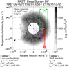 |
Fig. 3. Unstable electron distribution measured by FAST in the Earth auroral region (Ergun et al. 2000). This kind of distribution is typical in the auroral regions emitting radio emissions. It consists in a cold (a few eV) Gaussian distribution with a warmer (a few hundred eV) halo which is shifted in energy by a few keV and whose pitch angle is scattered due to magnetic mirroring. We assumed a distribution function of that kind in our modelling of the beaming angle from auroral cavities. Velocity dispersion, corresponding to the cold and halo temperature (ϵc and ϵh), and velocity shift, corresponding to the beam energy (ϵb), are shown. The resonant electron velocity (vr) and the equivalent “thermal” velocity (vth) are also shown. |
These modes differ by the angular frequency of the emission, deduced from the resonance equation (Eq. (7)). The perpendicular emission angular frequency is obtained using vr∥ = 0 and is always smaller than the cold electron cyclotron angular frequency:
 (8)
(8)
The emission angular frequency of the oblique mode is obtained from the centre of the circle tangent to the loss-cone boundary. The position of this resonance circle is related to resonant electrons pitch angle α (i.e. the loss-cone angle), which depends on the angular frequency:
 (9)
(9)
with ωcmax being the electron cyclotron angular frequency at the altitude below which the electrons are lost by collision with the planetary atmosphere.
Therefore, using Eqs. (5) and (9) to replace k∥ and vr∥, respectively, the resonant equation of Eq. (2) can be rewritten as
 (10)
(10)
Finally, using the fact that for resonant electron (Hess et al. 2008)
 (11)
(11)
we obtain (with a Taylor expansion and an inverse Taylor expansion for the final form)
 (12)
(12)
Contrary to perpendicular emission, oblique emission is emitted above the cold plasma electron cyclotron frequency. The difference in frequency between these modes has important consequences due to the characteristics of the dispersion relation of the right-handed waves in the plasma (Lassen 1926).
While the bulk electron velocity is zero in the plasma rest frame, the velocity of individual electrons is not zero. One therefore needs to introduce a Lorentz factor Γth into the refraction index expression, translating the non-zero velocity of the electrons in the plasma rest frame (Pritchett 1984; Louarn & Le Quéau 1996a). Exact computation of this relativistic correction may be complicated (Pritchett 1984), but it can be estimated by introducing an equivalent “thermal” velocity vth, meaning that the mean energy of the electrons in the plasma rest frame is  (Louarn & Le Quéau 1996a; Mottez et al. 2010). This relativistic term is of importance, as it participates – along with the ratio between the plasma and the electron cyclotron frequency (ωp/ωc) – in the determination of the mode(s) on which the waves can be emitted (or not).
Therefore, in a non-zero temperature plasma, the expression of the refraction index is
 (13)
(13)
 (14)
(14)
When the refractive index N tends to 1, the wave propagates through the plasma with the same characteristics as if it propagated in a vacuum. When the refractive index becomes very different from 1, the peculiarities of the wave propagation in the plasma are highlighted. For certain characteristic angular frequencies of the plasma, the refractive index may tend towards 0 or towards infinity. We then speak of cutoff frequency (N → 0) or resonant frequency (N → ∞), which defined the different modes. The cutoff angular frequencies are ωp and  . The resonant angular frequencies depend on θ. If θ = 0 then the resonant angular frequencies are ωp and Ωcth. If θ = π/2 then there is only one resonant angular frequency known as the upper hybrid angular frequency
  .
.
The modes discussed here all have pure circular polarization. Elliptically polarized waves amplified by the CMI can split in L−O (in green Fig. 4a) and R−X modes on index gradients (Melrose 1980; Shaposhnikov et al. 1997; Louarn & Le Quéau 1996b). In the following we only consider Right-Extraordinary emissions (i.e. the + sign Eq. (13)), because they are the dominant ones in most observed auroral emissions, and for that reason they are the only ones simulated by the ExPRES code so far.
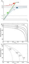 |
Fig. 4. Panel a: sketch of the dispersion relation of the electromagnetic waves in a plasma, following the Appleton-Hartree equation. Only R−X and L−O modes can escape the plasma and become radio waves. Panel b: beaming angle of the oblique emissions as a function of the ratio of the emission angular frequency to the maximal electron cyclotron angular frequency, for different values of the electrons energy and N = 1. Panel c: beaming angle of the perpendicular emissions as a function of ωp/ωc outside of a cavity. Symbols correspond to terrestrial auroral kilometric radiation (AKR) beaming angle measurements by Louarn & Le Quéau (1996b). Lines are theoretical beaming angles computed using Eqs. (20) and (25), constrained by density measurements of Louarn & Le Quéau (1996b) for orbit 176 (solid line), orbit 1260 (dashed), and orbit 165 (dot-dashed). |
Below the resonant angular frequency ω = ωUH the wave is on the Right-Extraordinary R−Z mode (in blue Fig. 4a, defined by the R mode propagating below ωc and the X mode propagating between ωL and ωUH), and above the cutoff angular frequency ω = ωR the wave is on the Right-Extraordinary R−X mode (in red Fig. 4a, defined by the R and X modes propagating above ωR). Only the R−X mode connects to the ω = ck dispersion relation of freely propagating radio waves (in black solid line Fig. 4a), whereas the R−Z mode is trapped inside its source region. Hence, R−X mode waves are the only RH waves observed as radio emissions (Louarn & Le Quéau 1996b). The “choice” of the CMI between the R−Z and R−X modes is determined by two factors: the wave angular frequency ω, which is constrained by the resonant electron velocity, and the cutoff angular frequency, which depends on ωp/ωc and vth. In the auroral regions the resonant angular frequency is always within a few percent of ωc. Lower values of ωp/ωc and/or higher values of vth lead to smaller values of the cutoff angular frequency – that can even lie below ωc –, whereas higher ωp/ωc and/or lower vth lead to larger cutoff frequencies.
ExPRES computes the cutoff frequency at each point of the user-defined radio source from Eq. (13), and the wave frequency from the electron velocity distribution (see Sect. 3.3), and considers that emission is produced only if the wave frequency is above the cutoff frequency. Thus, ExPRES needs to be fed with the local magnetic field strength (that defines ωc), the local plasma density (that defines ωp), and the mean energy of the electrons in the source (that defines vth).
4. Radiation pattern
4.1. Transient (Alfvénic) current system
In the case of a transient current system, electrons are accelerated by Alfvén wave electric fields, and a ring (Hess et al. 2007b) or a Kappa-like (Swift 2007) distribution is formed. Also, the Alfvén waves do not generate a deep auroral cavity devoid of cold plasma (Mottez et al. 2010). In these conditions, the oblique R−X mode is the one that will be favoured. Its beaming angle is obtained by solving Eqs. (13), (6), (11), and (12) simultaneously. First, the refraction index is obtained by equating the value of the centre of the resonance sphere v0 in Eqs. (6) and (11):
 (15)
(15)
The dispersion relation is obtained from the dielectric tensor (Stix 1962) and can be written as
 (16)
(16)
Setting  and using the resonance equation (Eq. (7)) and the notation of Stix (1962),
 (17)
(17)
and the coefficients of Eq. (16) can be rewritten to obtain a second-order equation in cos2 θ,
![Mathematical equation: $$ \begin{aligned} S\chi ^4+&\left[\chi ^4(P-S)-\chi ^2(PS+S^2-D^2)\right]\cos ^2\theta \nonumber \\ &+\left[P(S^2-D^2)-\chi ^2(PS-S^2+D^2)\right]\cos ^4\theta \\ &=a\cos ^4\theta +b\cos ^2\theta +c=0.\nonumber \end{aligned} $$](/articles/aa/full_html/2019/07/aa35161-19/aa35161-19-eq23.gif) (18)
(18)
The solution for the R−X mode is
 (19)
(19)
For a transient current system, the beaming angle inside the source computed by ExPRES is the exact solution of the above equation. To perform the calculation, ExPRES needs the user to specify the accelerated electron mean energy ( ) and the plasma temperature (
 ), whereas the ratio between plasma frequency and electron cyclotron frequency is deduced from the density profiles associated with the celestial bodies considered (see Sect. 2).
Figure 4b shows the evolution of the beaming angle as a function of the ratio between the emission angular frequency ω and the maximal cyclotron angular frequency reachable ωcmax for different resonant electron energies ϵ. The plasma angular frequency ωp was considered to be negligible in that case.
4.2. Steady-state current system
At the source, the beaming of the radio emissions generated by a steady-state current system is more simple than in the previous case: if the R−X mode can be amplified, waves are beamed perpendicular to the magnetic field. However, in the case of AKR at Earth, the emission is, most of the time, observed to be generated inside of a plasma cavity and to be refracted on its border (Louarn & Le Quéau 1996b,a). This leads to a very complex situation due to the fact that the beaming angle outside the cavity depends on the cavity profile. There is a wide variety of possible cavity profiles and very few constraints on them. Moreover, depending on the shape of the cavity, waves can be partially trapped and resonate inside the cavity, with an impact on the radio beaming. As a consequence, it is not possible to define an exact general solution to the problem of the beaming angle of a radio source inside a cavity. Even for a well-defined cavity profile, computation of the beaming requires a ray-tracing algorithm, which needs too much computational power to be integrated in ExPRES.
ExPRES therefore uses an approximate solution, assuming that the refraction mainly occurs inside the cavity and not on its borders. The need for refraction inside the source was already emphasised by Louarn & Le Quéau (1996a), and its existence is related to the presence of a gradient of refraction index inside the cavity due to the gradient of magnetic field strength. This gradient is mainly parallel to the magnetic field. Therefore, the major difference between ExPRES computation and reality is that ExPRES assumes that the wave reaches a region where the refraction index is N = 1 inside the source, in which case refraction on the cavity border has a low impact on the final beaming angle. In reality however a slight increase of the refraction index in the cavity allows the wave to escape it, meaning that a large part of the refraction takes place on the cavity border. We note that the assumption made in ExPRES is likely to be a good approximation in the case of a large cavity (in terms of its perpendicular size relative to the radio wavelength), because in that case a significant fraction of the refraction is indeed expected to take place inside the cavity. In such a large cavity, strong trapping of the wave is also unlikely, and thus no effect is expected on the radio beaming.
Under the above assumption, and considering that the index gradient is parallel to the magnetic field and using Snell-Descartes law, computation of the radio beaming angle becomes simply
 (20)
(20)
with the refraction index N being that of a pure X mode (purely perpendicular to the magnetic field) with ω = Ωcr, that is,
 (21)
(21)
It is clear from this equation that in order to have a real refraction index (permitting wave propagation), the electron mean energy (i.e. temperature) must be greater than the resonant electron mean energy, meaning that Γth > Γr and thus  .
.
Equation (21) is very sensitive to the variation of each parameter, and therefore the relation between them has to be set carefully from physical considerations relevant to the source considered. This is particularly the case for the electron distribution.
ExPRES models the unstable distribution as a bi-Maxwellian distribution at rest accelerated to a given energy. Thus, we define three characteristic electron energies: the beam energy (ϵb) which corresponds to the energy of accelerated electrons (usually several keV), the core thermal energy of the electron (ϵc) which is the temperature of the core of the distribution of the background electrons (usually a few eV to a few tens of eV), and the halo temperature of the electron (ϵh) which is the mean energy of supra-thermal electrons (usually a few hundred eV). The electron density inside the source is taken proportional to that outside of the source (i.e. that of the plasma before acceleration), with a proportionality coefficient deduced from current conservation (density × velocity is constant). The plasma angular frequency in the source is therefore deduced from the ratio between beam and core energies:
 (22)
(22)
The halo temperature is used to determine the resonant electron energy. This energy is not that of the beam, because the resonance circle of a shell-driven CMI passes through the region of largest ∇vr⊥f(vr), that is within the inner edge of the shell and not along the peak of the distribution. For a shifted-Maxwellian distribution of the energies in the beam (with a standard-deviation ϵh), the largest positive gradient is obtained for an energy ϵb − ϵh. Thus the difference between the mean and resonant energies of the electron is
 (23)
(23)
As noted in Mottez et al. (2010), using ϵc instead of ϵh would not permit the generation of an X-mode wave (the plasma needs to be hot), hence our assumption of the presence of a halo, which is usually observed at energies of a few hundred electronvolts in magnetospheric plasmas (Ergun et al. 2000).
Depending on what the user knows as physical parameters, two choices are possible with ExPRES. Either the user specifies the plasma density in the sources ωpsource, or only the global magnetospheric density (not direclty that of the sources).
In the former case (if the user knows ωpsource), using Eqs. (14) and (23), the refraction index of Eq. (21) becomes
 (24)
(24)
In the latter case (if the user does not know ωpsource), using Eq. (22) the refraction index of Eq. (21) then becomes
 (25)
(25)
Figure 4c displays the beaming angles computed using the above equation, with parameters η and ϵh deduced from measurements in terrestrial auroral cavities. The value of η was estimated from the densities inside (∼1 cm−3) and outside (deduced from measured fpe) of the cavities (Louarn & Le Quéau 1996b), and ϵh was taken to be ≃900 eV, consistent with the distributions measured by Ergun et al. (2000). With measured beam energies ϵb = 3−10 keV, the resonant energy of the electrons is about 2−9 keV. The modelled beaming curves are in good agreement with the observed values of the beaming angles (symbols) for the observations of AKR corresponding to the density measurements in Louarn & Le Quéau (1996b).
4.3. Refraction in the source vicinity
The refraction index has an important effect inside the source since the resonance process occurs close to the R−X mode cutoff angular frequency ωR, where the refraction index varies rapidly for small variation of the plasma parameters.
Outside of the source, the refraction index rapidly goes to one, in which case the waves escape freely as radio waves, or to zero, in which case the waves meet a reflection layer and are reflected. This phenomenon happens close to the source, where the local cyclotron angular frequency is still close to that inside the source (and thus close to the wave frequency).
This refraction effect outside the source differs from that inside the source by the fact that it is not symmetrical relative to the magnetic field vector (see e.g. Galopeau & Boudjada 2016, for Io). Indeed, if a wave is emitted toward decreasing ωc, it will encounter its cutoff angular frequency ωR, and will then be refracted. The ExPRES code models the refraction effect outside the source under the approximation of planar refraction index iso-surfaces (iso-ωc) close to the source, with a refraction index varying only in the local meridian plane. Thus the gradient of refraction index is assumed to be null in the longitudinal direction, meaning that the normal to the refraction index planes has a null longitudinal component. The modification of the beaming angle is then obtained easily from the Snell-Descartes law.
5. Simulation results, code accessibility, limitations and perspectives
5.1. Versions of ExPRES
Each version of the code has had new modules added and minor bugs fixed. The majors evolutions are summarised here.
The first versions (0.1, 0.2 and 0.3) of the ExPRES code were developed to predict and interpret the current observations of the NASA Juno space mission to Jupiter. Indeed, the previous low-frequency radio astronomy experiments (such as Cassini/RPWS, Gurnett et al. 2004) were able to measure the four Stokes parameters and the k vector of incoming waves (Cecconi et al. 2009). In the case of Juno (Bagenal et al. 2017; Bolton et al. 2017), the radio experiment onboard (named Waves, Kurth et al. 2017) only measures the total intensity of incoming radio waves versus time and frequency (it also performs some limited direction-finding, but that proved effective for case studies Imai et al. 2017). The development of the ExPRES tool was therefore necessary to determine the origin of the emissions. Version 0.4 of the code allowed a generalization to Saturn and version 0.5 to exoplanets. For version 0.6, the code architecture was completely redesigned and the production of 3D movies was added. The current stable version is 1.0 and allows simulation results to be produced in CDF (Space Physics Data Facility 2018) from JSON formatted (Bray 2017) input files.
5.2. Output parameters
Different output parameters can be selected. The default setup returns the following information at each time and frequency step.
-
Polarization: degree of circular polarization of the observed wave (if it is detected), making it possible to differentiate emission from the northern (<0) or the southern hemisphere (>0);
-
Theta: opening of the conical emission sheet;
-
CML: central meridian longitude, that is the west jovicentric longitude of the observer;
-
ObsLatitude: planetocentric latitude of the observer;
-
ObsDistance: distance (in planetary radius) between the observer and the planet;
-
SrcFreqMax: maximum frequency on the active flux tube at each time step;
-
Fp: electronic plasma frequency inside the visible sources;
-
Fc: electronic cyclotron frequency inside the visible sources.
Additional information may be requested by the user, such as:
-
The azimuth ϕ of the wave seen by the observer, that is the part of the conical emission sheet from which the wave seen by the observer comes from.
-
The equatorial longitude crossing with the active magnetic field line. For simulations of emissions induced by a moon, the longitude of the sources is the longitude of the moon.
-
The position (x, y, z) of the sources.
5.3. Simulation results
Figure 5 shows observations with the Nançay Decameter Array (NDA) of the Io-controlled Jovian emissions of type A (Fig. 5a), B (Fig. 5b), C (Fig. 5e), and D (Fig. 5f). Figures 5a and b display the right-handed polarization observation of the NDA (thus emission coming from the northern hemisphere) while Figs. 5e and f display the left-handed polarization observations (thus emission coming from the southern hemisphere). These emissions can be modelled using ExPRES. The corresponding simulated dynamic spectra are plotted under each NDA observation. The simulations matching best the observations are obtained assuming emissions from magnetic field line connected to the Io Main Alfvén Wing footprint, using the JRM09 magnetic field model (Connerney et al. 2018), completed by the current sheet model of Connerney et al. (1993), and electrons with energies of 11 keV (Io-A, Fig. 5c), 2.5 keV (Io-B, Fig. 5d), 9 keV (Io-C, Fig. 5g), and 8 keV (Io-D, Fig. 5h). The slight uncertainty in time (of the order of 1 min) and in frequency (of the order of kHz) comes from the fact that the active flux tube location (connected to the Io Main Alfvén Wing footprint) is not absolutely known (here is used the simple sinusoidal model of Hess et al. 2011).
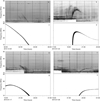 |
Fig. 5. Panels a, b, e, f: examples of Io-controlled jovian radio emissions (of type A, B, C, D, respectively) observed by the NDA. Right-handed (panels a and b) and left-handed (panels e and f) polarization are separated. Panels c, d, g, h: corresponding ExPRES simulated dynamic spectra are computed using the JRM09 model (Connerney et al. 2018), completed by the Connerney et al. (1993) current sheet model, and assuming a source originating from the magnetic field line connected to the main Io Alfvén wing spot on Jupiter and electrons with energies (ϵb) of 11 keV (c), 2.5 keV (d), 9 keV (g) and 8 keV (h), respectively. |
ExPRES has already been used to model observations, attempting to reproduce the time-frequency morphology of the radio emissions from Saturn (Lamy et al. 2008, 2011, 2013). ExPRES allowed the authors to discover subcorotating field-aligned current systems and to put constraints on the energy of the accelerated electrons involved in the auroral radio emission, with energies of the order of a few tens of kiloelectronvolts, consistent with UV observations.
ExPRES has also been used to model observations and reproduce time-frequency morphology of the radio emissions from Jupiter (Hess et al. 2008, 2011, 2010a; Ray & Hess 2008). It allowed the authors to determine the localization of the Io-Jupiter current circuit (downstream of the instantaneous Io-Jupiter field line). As in the studies of Saturn, ExPRES allowed the authors to find that accelerated electrons of a few kiloelectronvolts are involved in the auroral radio emissions.
To predict and interpret radio emission from Jupiter, ExPRES simulations were performed using a predefined dataset for the input parameters (based on the parametric study of Louis et al. 2017c, using Juno/Waves and Voyager/PRA data). This allowed the authors to detect radio emissions induced by Europa and Ganymede using Cassini/RPWS and Voyager/PRA data (Louis et al. 2017a) and interpret the time-frequency morphology of Juno/Waves observations (Louis et al. 2017b, which was the initial goal of the code).
ExPRES was similarly used to simulate the radio environment of the Jupiter Icy Moon Explorer (JUICE) spacecraft planned to be sent to Jupiter by ESA, in order to estimate how much the natural radio emissions from Jupiter’s magnetosphere below 40 MHz would pollute the spacecraft radar measurements in the range 5−50 MHz (Cecconi et al. 2012).
Finally, Hess & Zarka (2011) discussed how the morphology of the radio emissions from exoplanetary magnetospheres or star–planet systems (involving plasma or magnetic interactions) could be interpreted to derive the magnetic field strength and the rotation period of the emitting body (planet or star), its orbital period, its orbital inclination, and the magnetic field tilt relative to its rotation axis or the offset relative to the centre of the planet. For most of these parameters, radio observations provide a unique means of measuring them.
5.4. Accessibility
The ExPRES code is written in IDL1. The code is available under MIT licence on GitHub within the MASER2 library repository3. The current version of the ExPRES code (V1.0) has been validated using IDL version 8.4.
Precomputed ExPRES simulation runs are available through different interfaces described on the MASER project (Cecconi et al. 2018a,b) website4: (i) a web directory listing access; (ii) a virtual observatory access using the EPN-TAP (Erard et al. 2018); and (iii) a streaming access using the das2 server framework (Piker 2017) through the MASER das2 server. Table 1 provides URLs for all access interfaces.
Access interfaces for ExPRES precomputed dataset.
The ExPRES code is also available for run-on-demand operations5. This computing interface requires an ExPRES JSON input configuration file. Examples of such configuration files are available through the web directory listing or virtual observatory catalogue: each of the precomputed files is provided with its input configuration file. The JSON input files must conform to the corresponding JSON-schema specification, the current version of which is available online6.
5.5. Limitations
The main limitations of the ExPRES code are listed below.
– ExPRES only models radio waves on the Right-Handed Extraordinary propagation modes, that is, the R−X and Z modes, the second being trapped in the source. The R−X is dominant in the observations. Modelling the Left-Handed Ordinary (L−O) mode (in green Fig. 4) requires the index of refraction N (Eq. (13)) to be modified, by choosing the − sign.
– ExPRES does not contain a ray-tracing algorithm. The code takes into account the refraction in the source region (e.g. in the auroral cavity if there is any) and in the source vicinity (see Sects. 4.2 and 4.3). The refraction far from the sources (e.g. in the equatorial plasma sheet for the lower-frequency emissions) is not modelled. The connection with the ARTEMIS-P (Anisotropic Ray Tracer for Electromagnetism in Magnetosphere, Ionosphere and Solar wind including Polarization) ray-tracing code (Gautier et al. 2013) will be studied in the future.
– ExPRES does not compute the growth rate of the radio source. Hence, the simulation cannot provide the intensity of the emission. ExPRES is an occurrence prediction tool. It predicts when an observer can observe a radio source if it is active at this time.
5.6. Perspectives
ExPRES has proven to be a very useful tool for the modelling, analysis, and interpretation of Jupiter and Saturn radio emissions, the preparation and operation of planetary missions, and for the current observations programs searching for exoplanetary radio emissions. Such detections are expected soon as a result of extensive observing programs with giant radio telescopes such as LOFAR (LOw Frequency ARray, van Haarlem et al. 2013), UTR2 (Ukrainian T-shaped Radio telescope, Braude et al. 1978), GMRT (Giant Metrewave Radio Telescope, Swarup 1991), NenuFAR (New Extension in Nançay Upgrading loFAR, Zarka et al. 2012) and ultimately SKA (Square Kilometre Array, Zarka et al. 2015; Acero et al. 2017).
Future uses will include the modelling of the time-frequency morphology of Jovian hectometer and broadband kilometer emissions (Boischot et al. 1981), the modelling of the longitude-frequency morphology of Jovian hectometer, and Io-independent decameter emissions (Imai et al. 2008, 2011). ExPRES will also be used to search for radio emissions induced by the kronian moons, such as Titan (potentially inducing radio emissions, Menietti et al. 2007) or Enceladus (which induces UV emissions at its footprint, Pryor et al. 2011). The code will also be used to simulate the radio emission of the Ice Giants (Warwick et al. 1986, 1989), or to predict potential radio emission from Mercury that would be observed by the BepiColombo/MMO/PWI instrument (Plasma Wave Investigation Kasaba et al. 2010).
Interactive Data Language, Exelis Visual Information Solutions, Boulder, Colorado.
Measuring, Analyzing and Simulating Emissions in the Radio range.
ExPRES page on the MASER website: http://maser.lesia.obspm.fr/tools-services-6/expres
Acknowledgments
Versions 0.1 to 0.5 of ExPRES were developed as SERPE (Simulateur d’Émissions Radio Planétaires et Exoplanétaires in French) by the LESIA laboratory under Observatoire de Paris and CNRS funding. Version 0.6.0 was developed by S. L. G. Hess on his own resources and with support from the LESIA, Observatoire de Paris for the online services. Later versions, including the current 1.0.0 version, were developed by the MASER team (http://maser.lesia.obspm.fr) which gathers personnel and funding from CNRS, CNES and Observatoire de Paris. Technical support from PADC (Paris Astronomical Data Center) is also acknowledged, with the very helpful contribution of P. Le Sidaner (DIO, Observatoire de Paris) and M. Servillat (LUTh, Observatoire de Paris). The Nançay Decamater Array acknowledges the support from the Programme National de Planétologie and the Programme National Soleil-Terre of CNRS-INSU. S. L. G. Hess thanks the MOP team of the LASP (Colorado Univ. Boulder) and R. Modolo (LATMOS/CNRS) for scientific support and fruitful comments. C.L. acknowledges funding from the CNES and from the LABEX Plas@par project and the Agence Nationale de la Recherche (as part of the program Investissements d’Avenir under the reference ANR-11-IDEX-0004-02). Part of the data distribution setup has been done in the frame of the Europlanet H2020 Research Infrastructure project, which has received funding from the European Union’s Horizon 2020 research and innovation programme under grant agreement No 654208. The authors thank the referee for fruitful comments and the careful reading of the manuscript.
References
- Acero, F., Acquaviva, J. T., Adam, R., et al. 2017, ArXiv e-prints [arXiv:1712.06950] [Google Scholar]
- Axford, W. I., & Hines, C. O. 1961, Can. J. Phys., 39, 1433 [NASA ADS] [CrossRef] [Google Scholar]
- Bagenal, F., Adriani, A., Allegrini, F., et al. 2017, Space Sci. Rev., 213, 219 [NASA ADS] [CrossRef] [Google Scholar]
- Boischot, A., Lecacheux, A., Kaiser, M. L., et al. 1981, J. Geophys. Res., 86, 8213 [NASA ADS] [CrossRef] [Google Scholar]
- Bolton, S. J., Lunine, J., Stevenson, D., et al. 2017, Space Sci. Rev., 213, 5 [NASA ADS] [CrossRef] [Google Scholar]
- Braude, S. I., Megn, A. V., Riabov, B. P., Sharykin, N. K., & Zhuk, I. N. 1978, Ap&SS, 54, 3 [NASA ADS] [CrossRef] [Google Scholar]
- Bray, T. 2017, The JavaScript Object Notation (JSON) Data Interchange Format, Tech. Rep. RFC 8259, IETF [CrossRef] [Google Scholar]
- Cecconi, B., Lamy, L., Zarka, P., et al. 2009, J. Geophys. Res. (Space Phys.), 114, A03215 [NASA ADS] [Google Scholar]
- Cecconi, B., Hess, S., Hérique, A., et al. 2012, Planet. Space Sci., 61, 32 [NASA ADS] [CrossRef] [Google Scholar]
- Cecconi, B., Le Sidaner, P., Savalle, R., et al. 2018a, PV-2018 Conference Proceedings, 20 [Google Scholar]
- Cecconi, B., Loh, A., Le Sidaner, P., et al. 2018b, Earth and Space Science Open Archive, https://www.essoar.org/doi/pdf/10.1002/essoar.10500145.1 [Google Scholar]
- Connerney, J. E. P., Baron, R., Satoh, T., & Owen, T. 1993, Science, 262, 1035 [NASA ADS] [CrossRef] [Google Scholar]
- Connerney, J. E. P., Kotsiaros, S., Oliversen, R. J., et al. 2018, Geophys. Res. Lett., 45, 2590 [NASA ADS] [CrossRef] [Google Scholar]
- Cowley, S. W. H., & Bunce, E. J. 2001, Planet. Space Sci., 49, 1067 [NASA ADS] [CrossRef] [Google Scholar]
- Delamere, P. A., & Bagenal, F. 2010, J. Geophys. Res. (Space Phys.), 115, 10201 [NASA ADS] [Google Scholar]
- Dungey, J. W. 1961, Phys. Rev. Lett., 6, 47 [NASA ADS] [CrossRef] [Google Scholar]
- Erard, S., Cecconi, B., Le Sidaner, P., et al. 2018, Planet. Space Sci., 150, 65 [Google Scholar]
- Ergun, R. E., Carlson, C. W., McFadden, J. P., et al. 2000, ApJ, 538, 456 [NASA ADS] [CrossRef] [Google Scholar]
- Faden, J., Weigel, R. S., Merka, J., & Friedel, R. H. W. 2010, Earth Sci. Inform., 3, 41 [CrossRef] [Google Scholar]
- Galopeau, P. H. M., & Boudjada, M. Y. 2016, J. Geophys. Res. (Space Phys.), 121, 3120 [NASA ADS] [CrossRef] [Google Scholar]
- Gautier, A. L., Cecconi, B., & Zarka, P. 2013, Journées Scientifiques URSI-France 26/27 mars 2013, 1 [Google Scholar]
- Genova, F., & Aubier, M. G. 1985, A&A, 150, 139 [NASA ADS] [Google Scholar]
- Gurnett, D. A., & Goertz, C. K. 1981, J. Geophys. Res. (Space Phys.), 86, 717 [NASA ADS] [CrossRef] [Google Scholar]
- Gurnett, D. A., Kurth, W. S., Kirchner, D. L., et al. 2004, Space Sci. Rev., 114, 395 [NASA ADS] [CrossRef] [Google Scholar]
- Hess, S. L. G., & Zarka, P. 2011, A&A, 531, A29 [NASA ADS] [CrossRef] [EDP Sciences] [Google Scholar]
- Hess, S., Zarka, P., & Mottez, F. 2007a, Planet. Space Sci., 55, 89 [NASA ADS] [CrossRef] [Google Scholar]
- Hess, S., Mottez, F., & Zarka, P. 2007b, J. Geophys. Res., 112, A11212 [NASA ADS] [CrossRef] [Google Scholar]
- Hess, S., Cecconi, B., & Zarka, P. 2008, Geophys. Res. Letter, 35, 13107 [NASA ADS] [CrossRef] [Google Scholar]
- Hess, S., Pétin, A., Zarka, P., Bonfond, B., & Cecconi, B. 2010a, Planet. Space Sci., 58, 1188 [NASA ADS] [CrossRef] [Google Scholar]
- Hess, S. L. G., Delamere, P., Dols, V., Bonfond, B., & Swift, D. 2010b, J. Geophys. Res. (Space Phys.), 115, 6205 [NASA ADS] [Google Scholar]
- Hess, S. L. G., Bonfond, B., Zarka, P., & Grodent, D. 2011, J. Geophys. Res., 116, A05217 [NASA ADS] [CrossRef] [Google Scholar]
- Hess, S. L. G., Echer, E., Zarka, P., Lamy, L., & Delamere, P. A. 2014, Planet. Space Sci., 99, 136 [NASA ADS] [CrossRef] [Google Scholar]
- Hill, T. W., Dessler, A. J., & Michel, F. C. 1974, Geophys. Res. Lett., 1, 3 [NASA ADS] [CrossRef] [Google Scholar]
- Imai, M., Imai, K., Higgins, C. A., & Thieman, J. R. 2008, Geophys. Res. Lett., 35, 17103 [NASA ADS] [CrossRef] [Google Scholar]
- Imai, M., Imai, K., Higgins, C. A., & Thieman, J. R. 2011, J. Geophys. Res. (Space Phys.), 116, 12233 [Google Scholar]
- Imai, M., Kurth, W. S., Hospodarsky, G. B., et al. 2017, Geophys. Res. Lett., 44, 6508 [NASA ADS] [CrossRef] [Google Scholar]
- Kaiser, M. L., Zarka, P., Kurth, W. S., Hospodarsky, G. B., & Gurnett, D. A. 2000, J. Geophys. Res., 105, 16053 [NASA ADS] [CrossRef] [MathSciNet] [Google Scholar]
- Kasaba, Y., Bougeret, J.-L., Blomberg, L. G., et al. 2010, Planet. Space Sci., 58, 238 [NASA ADS] [CrossRef] [Google Scholar]
- Kurth, W. S., Baumback, M. M., & Gurnett, D. A. 1975, J. Geophys. Res., 80, 2764 [NASA ADS] [CrossRef] [Google Scholar]
- Kurth, W. S., Hospodarsky, G. B., Kirchner, D. L., et al. 2017, Space Sci. Rev., 213, 347 [NASA ADS] [CrossRef] [Google Scholar]
- Kuznetsov, A. A., Doyle, J. G., Yu, S., et al. 2012, ApJ, 746, 99 [NASA ADS] [CrossRef] [Google Scholar]
- Ladreiter, H. P., Zarka, P., & Lacacheux, A. 1994, Planet. Space Sci., 42, 919 [NASA ADS] [CrossRef] [Google Scholar]
- Lamy, L., Zarka, P., Cecconi, B., Hess, S., & Prangé, R. 2008, J. Geophys. Res. (Space Phys.), 113, 10213 [NASA ADS] [CrossRef] [Google Scholar]
- Lamy, L., Cecconi, B., Zarka, P., et al. 2011, J. Geophys. Res. (Space Phys.), 116, A04212 [NASA ADS] [CrossRef] [Google Scholar]
- Lamy, L., Prangé, R., Pryor, W., et al. 2013, J. Geophys. Res. (Space Phys.), 118, 4817 [NASA ADS] [CrossRef] [Google Scholar]
- Lamy, L., Zarka, P., Cecconi, B., et al. 2018, Science, 362, aat2027 [NASA ADS] [CrossRef] [Google Scholar]
- Lassen, H. 1926, I. Zeitschrift für Hochfrequenztechnik, 28, 109 [Google Scholar]
- Lecacheux, A., Boudjada, M. Y., Rucker, H. O., et al. 1998, A&A, 329, 776 [NASA ADS] [Google Scholar]
- Louarn, P. 1992, Adv. Space Res., 12, 121 [CrossRef] [PubMed] [Google Scholar]
- Louarn, P., & Le Quéau, D. 1996a, Planet. Space Sci., 44, 211 [NASA ADS] [CrossRef] [Google Scholar]
- Louarn, P., & Le Quéau, D. 1996b, Planet. Space Sci., 44, 199 [NASA ADS] [CrossRef] [Google Scholar]
- Louarn, P., Allegrini, F., McComas, D. J., et al. 2017, Geophys. Res. Lett., 44, 4439 [NASA ADS] [CrossRef] [Google Scholar]
- Louis, C. K., Lamy, L., Zarka, P., Cecconi, B., & Hess, S. L. G. 2017a, J. Geophys. Res. (Space Phys.), 122, 9228 [Google Scholar]
- Louis, C. K., Lamy, L., Zarka, P., et al. 2017b, Geophys. Res. Lett., 44, 9225 [NASA ADS] [CrossRef] [Google Scholar]
- Louis, C. K., Lamy, L., Zarka, P., et al. 2017c, in Planetary Radio Emissions VIII, ed. G. Fisher, et al. (Vienna: Austrian Academy of Sciences Press), 59 [Google Scholar]
- Matsuda, K., Terada, N., Katoh, Y., & Misawa, H. 2012, J. Geophys. Res. (Space Phys.), 117, 10214 [NASA ADS] [CrossRef] [Google Scholar]
- Melrose, D. B. 1980, Plasma Astrophysics (New York: Gordon and Breach) [Google Scholar]
- Menietti, J. D., Groene, J. B., Averkamp, T. F., et al. 2007, J. Geophys. Res. (Space Phys.), 112, A08211 [NASA ADS] [CrossRef] [Google Scholar]
- Mottez, F., Hess, S., & Zarka, P. 2010, Planet. Space Sci., 58, 1414 [NASA ADS] [CrossRef] [Google Scholar]
- Mutel, R. L., Gurnett, D. A., Christopher, I. W., Pickett, J. S., & Schlax, M. 2003, J. Geophys. Res. (Space Phys.), 108, 1398 [NASA ADS] [CrossRef] [Google Scholar]
- Neubauer, F. M. 1980, J. Geophys. Res., 85, 1171 [Google Scholar]
- Panchenko, M. 2003, Radio Sci., 38 [Google Scholar]
- Panchenko, M., & Rucker, H. O. 2016, A&A, 596, A18 [NASA ADS] [CrossRef] [EDP Sciences] [Google Scholar]
- Piker, C. 2017, Das2 Version 2.2.2 Interface Reference, Tech. Rep. (University of Iowa) [Google Scholar]
- Pottelette, R., & Pickett, J. 2007, Nonlinear Process. Geophys., 14, 735 [NASA ADS] [CrossRef] [Google Scholar]
- Pritchett, P. L. 1984, J. Geophys. Res., 89, 8957 [NASA ADS] [CrossRef] [Google Scholar]
- Pryor, W. R., Rymer, A. M., Mitchell, D. G., et al. 2011, Nature, 472, 331 [NASA ADS] [CrossRef] [Google Scholar]
- Queinnec, J., & Zarka, P. 1998, J. Geophys. Res., 103, 26649 [NASA ADS] [CrossRef] [Google Scholar]
- Ray, L. C., & Hess, S. 2008, J. Geophys. Res., 113, A11218 [NASA ADS] [Google Scholar]
- Saur, J., Neubauer, F. M., Connerney, J. E. P., Zarka, P., & Kivelson, M. G. 2004, Plasma Interaction of Io with its Plasma Torus, Jupiter: The Planet, Satellites and Magnetosphere (Cambridge Planetary Science), 537 [Google Scholar]
- Shaposhnikov, V. E., Kocharovsky, V. V., Kocharovsky, V. V., et al. 1997, A&A, 326, 386 [NASA ADS] [Google Scholar]
- Space Physics Data Facility 2018, Common Data Format, NASA-GSFC, version 3.7.0 [Google Scholar]
- Stix, T. H. 1962, The Theory of Plasma Waves (New York: McGraw-Hill) [Google Scholar]
- Su, Y. J., Ma, L., Ergun, R. E., Pritchett, P. L., & Carlson, C. W. 2008, J. Geophys. Res. (Space Phys.), 113, 8214 [NASA ADS] [CrossRef] [Google Scholar]
- Swarup, G. 1991, in IAU Colloq. 131: Radio Interferometry: Theory, Techniques, and Applications, eds. T. J. Cornwell, & R. A. Perley, ASP Conf. Ser., 19, 376 [Google Scholar]
- Swift, D. W. 2007, J. Geophys. Res. (Space Phys.), 112, 12207 [NASA ADS] [Google Scholar]
- Treumann, R. A. 2006, A&ARv, 13, 229 [NASA ADS] [CrossRef] [Google Scholar]
- van Haarlem, M. P., Wise, M. W., Gunst, A. W., et al. 2013, A&A, 556, A2 [NASA ADS] [CrossRef] [EDP Sciences] [Google Scholar]
- Warwick, J. W., Evans, D. R., Romig, J. H., et al. 1986, Science, 233, 102 [NASA ADS] [CrossRef] [PubMed] [Google Scholar]
- Warwick, J. W., Evans, D. R., Peltzer, G. R., et al. 1989, Science, 246, 1498 [NASA ADS] [CrossRef] [Google Scholar]
- Wu, C. S. 1985, Space Sci. Rev., 41, 215 [NASA ADS] [CrossRef] [Google Scholar]
- Zarka, P. 1998, J. Geophys. Res., 103, 20159 [NASA ADS] [CrossRef] [Google Scholar]
- Zarka, P. 2004, Adv. Space Res., 33, 2045 [NASA ADS] [CrossRef] [Google Scholar]
- Zarka, P., Girard, J. N., Tagger, M., & Denis, L. 2012, in SF2A-2012: Proceedings of the Annual meeting of the French Society of Astronomy and Astrophysics, eds. S. Boissier, P. de Laverny, N. Nardetto, et al., 687 [Google Scholar]
- Zarka, P., Lazio, T. J. W., & Hallinan, G. 2015, Advancing Astrophysics with the Square Kilometre Array [Google Scholar]
All Tables
All Figures
|
Fig. 1. Panels a and b: examples of time-frequency radio arcs. Panel a: radio arcs emitted by the Io-Jupiter interaction (Queinnec & Zarka 1998), observed by Wind (0–15 MHz) and the Nançay Decameter Array (15–40 MHz). Panel b: radio arcs at Saturn, observed by Cassini, related to a sub-corotating hot spot in the magnetosphere of Saturn (Lamy et al. 2008). Panels c and d: side and polar views of the emission geometry, with two sources located along the same magnetic field line but at different altitudes. Arrows show the direction of propagation of the radio waves which can be seen by an observer located in the equatorial plane far from the planet. Panels e: dynamic spectrum of the emissions which would correspond to the geometry of panels c and d. |
| In the text | |
|
Fig. 2. Examples of the geometry involved in the modelling of the Io-controlled emissions of Jupiter. The emission depends on the relative position of Io, Jupiter, and the observer, in particular on the jovigraphic longitude of the observer (λCML, i.e. the central meridian longitude) and that of the active field line which can differ from that of Io (λIo) by a lead angle (δλ). |
| In the text | |
|
Fig. 3. Unstable electron distribution measured by FAST in the Earth auroral region (Ergun et al. 2000). This kind of distribution is typical in the auroral regions emitting radio emissions. It consists in a cold (a few eV) Gaussian distribution with a warmer (a few hundred eV) halo which is shifted in energy by a few keV and whose pitch angle is scattered due to magnetic mirroring. We assumed a distribution function of that kind in our modelling of the beaming angle from auroral cavities. Velocity dispersion, corresponding to the cold and halo temperature (ϵc and ϵh), and velocity shift, corresponding to the beam energy (ϵb), are shown. The resonant electron velocity (vr) and the equivalent “thermal” velocity (vth) are also shown. |
| In the text | |
|
Fig. 4. Panel a: sketch of the dispersion relation of the electromagnetic waves in a plasma, following the Appleton-Hartree equation. Only R−X and L−O modes can escape the plasma and become radio waves. Panel b: beaming angle of the oblique emissions as a function of the ratio of the emission angular frequency to the maximal electron cyclotron angular frequency, for different values of the electrons energy and N = 1. Panel c: beaming angle of the perpendicular emissions as a function of ωp/ωc outside of a cavity. Symbols correspond to terrestrial auroral kilometric radiation (AKR) beaming angle measurements by Louarn & Le Quéau (1996b). Lines are theoretical beaming angles computed using Eqs. (20) and (25), constrained by density measurements of Louarn & Le Quéau (1996b) for orbit 176 (solid line), orbit 1260 (dashed), and orbit 165 (dot-dashed). |
| In the text | |
|
Fig. 5. Panels a, b, e, f: examples of Io-controlled jovian radio emissions (of type A, B, C, D, respectively) observed by the NDA. Right-handed (panels a and b) and left-handed (panels e and f) polarization are separated. Panels c, d, g, h: corresponding ExPRES simulated dynamic spectra are computed using the JRM09 model (Connerney et al. 2018), completed by the Connerney et al. (1993) current sheet model, and assuming a source originating from the magnetic field line connected to the main Io Alfvén wing spot on Jupiter and electrons with energies (ϵb) of 11 keV (c), 2.5 keV (d), 9 keV (g) and 8 keV (h), respectively. |
| In the text | |
Current usage metrics show cumulative count of Article Views (full-text article views including HTML views, PDF and ePub downloads, according to the available data) and Abstracts Views on Vision4Press platform.
Data correspond to usage on the plateform after 2015. The current usage metrics is available 48-96 hours after online publication and is updated daily on week days.
Initial download of the metrics may take a while.