| Issue |
A&A
Volume 690, October 2024
|
|
|---|---|---|
| Article Number | A96 | |
| Number of page(s) | 7 | |
| Section | The Sun and the Heliosphere | |
| DOI | https://doi.org/10.1051/0004-6361/202348081 | |
| Published online | 01 October 2024 | |
Effect of temperature anisotropy formed by fast electron beams moving in the flare loop on its excited electron-cyclotron maser instability
1
College of Engineering, Lishui University, Lishui 323000, China
2
State Key Laboratory of Space Weather, National Space Science Center, Chinese Academy of Sciences, Beijing 100190, China
3
Key Laboratory of Planetary Sciences, Purple Mountain Observatory, CAS, Nanjing 210023, China
Received:
27
September
2023
Accepted:
30
July
2024
Abstract
Context. The electron-cyclotron maser instability (ECMI) is a significant coherent radio emission mechanism widely utilized in various astrophysical radio phenomena. It is well known that the velocity anisotropic distribution of energetic electrons, which leads to an inverted perpendicular population in the vertical direction with ∂fb/∂v⊥ > 0, can provide the free energy necessary for the ECMI.
Aims. The initial velocity distribution of energetic electrons leaving the acceleration region is typically isotropic or beam-like. However, as these energetic electrons travel along the magnetic field as fast electron beams (FEBs) in magnetic plasma, various velocity anisotropic distributions can emerge. In this paper, we examine the impact of temperature anisotropy formed by beam electrons traveling along a flare loop on the ECMI.
Methods. By neglecting the energy loss of energetic electrons as they traverse the corona and invoking the conservation of energy and magnetic moments, we established the relationship between momentum dispersion and the magnetic field. Utilizing the magnetic field model of the flare loop, we calculated the evolution of momentum dispersion and the growth rates of the ECMI as FEBs precipitate along the flare loop.
Results. The results demonstrate that the temperature anisotropy arising as FEBs descend along the flare loop significantly impacts the ECMI. The maximum growth rates of the excited modes exhibit a gradual increase initially and then decline rapidly after reaching a critical height for β0 = 0.2c and 0.15c. The results also show that the growth rates of the O2 mode are one order of magnitude smaller than those of the O1 and X2 modes. This indicates that the harmonic radiation is X-mode polarized. Notably, the temperature anisotropy of FEBs as they precipitate along the flare loop with different magnetic field models or at different heights has similar effects on the ECMI.
Key words: instabilities / masers / radiation mechanisms: non-thermal / Sun: radio radiation
Corresponding author; This email address is being protected from spambots. You need JavaScript enabled to view it. .
© The Authors 2024
 Open Access article, published by EDP Sciences, under the terms of the Creative Commons Attribution License (https://creativecommons.org/licenses/by/4.0), which permits unrestricted use, distribution, and reproduction in any medium, provided the original work is properly cited.
This article is published in open access under the Subscribe to Open model. This email address is being protected from spambots. You need JavaScript enabled to view it. to support open access publication.
1. Introduction
The electron-cyclotron maser instability (ECMI) is one of the coherent radiation processes that produces radio emission. Since Wu & Lee (1979) recognized the significance of the relativistic resonance condition and explained auroral kilometer radiation (AKR) with the loss cone ECMI model, this coherent mechanism has been widely applied to radio emissions from magnetized planets (Hewitt et al. 1981; Zarka 1998; Hess et al. 2007); solar radio bursts (SRBs), including type III radio bursts (Wu et al. 2002; Yoon et al. 2002; Zhao et al. 2013), type IV radio bursts, and fine structure (Wang 2004; Aschwanden & Benz 1988; Treumann et al. 2011); and solar radio spikes (Melrose & Dulk 1982; Aschwanden 1990b; Vlasov et al. 2002). Earlier theories suggested that the ECMI was excited by various velocity anisotropic distributions of energetic electrons, such as loss-cone distributions (Wu & Lee 1979; Melrose & Dulk 1982), temperature anisotropic distributions (Melrose 1976), and shell or horseshoe distributions (Bingham et al. 2004; Ergun et al. 2000). These different velocity anisopropic distributions manifest an inverted perpendicular population where ∂fb/∂v⊥ > 0 provides free energy for the ECMI. Another effective driving source of the ECMI is the lower energy cutoff behavior of power-law electrons (Wu & Tang 2008; Tang & Wu 2009).
In previous literature, the fast electron beams (FEBs) that excite the ECMI have typically been treated as an invariant source. However, as FEBs travel along magnetic fields in the solar atmosphere, their distribution can undergo changes due to various factors. For instance, energetic electrons may lose some of their energy due to collisional or non-collisional causes (Pick & van den Oord 1990; Tang et al. 2016), resulting in changes to the energy spectrum of FEBs. Tang et al. (2020, 2023) investigated the evolution of the energy spectrum as FEBs propagate in the solar atmosphere. Their findings indicate significant changes in the energy spectral parameters of FEBs due to energy loss, and these alterations can have important effects on the maser instability.
On the other hand, velocity anisopropic distributions can be generated when FEBs travel in the direction of increasing magnetic field strength (Melrose 1973). The well-studied loss-cone anisotropic distributions arise when energetic electron beams precipitate along converging magnetic fields (Wu & Lee 1979; Melrose & Dulk 1982; Aschwanden 1990a; Conway & Willes 2000). Melrose & Wheatland (2016) investigated spike bursts with the ECMI model and indicated that the horseshoe distribution can indeed form in a flare loop when beam-like electrons travel downward under plausible assumptions.
Another important anisotropic distribution is temperature anisotropy, which has been extensively studied by various authors (Melrose 1973, 1976; ŠtveráK et al. 2008; Camporeale & Burgess 2010; Tang et al. 2011). Temperature anisotropy can be formed by the betatron effect, which transforms parallel energy into perpendicular energy. Melrose (1973, 1976) used a bi-Maxwell electron distribution function to investigate coherent gyromagnetic emission and explain Jupiter’s decametric radiation. Due to non-relativistic resonance conditions, very high temperature anisotropies are required. Tang et al. (2011) discussed the effects of temperature anisotropy on the ECMI excited by lower energy cutoff behavior of power-law electrons, considering arbitrary temperature anisotropy parameters.
In this paper, we focus on the influence of temperature anisotropy, which arises during the propagation of FEBs in the flare loop, on the ECMI. We propose that the FEBs that excite the ECMI are accelerated at the flare loop top, initially exhibiting a power-law energy distribution, and travel downward along the flare loop after leaving the acceleration region. The calculation results from Tang et al. (2020) indicate that the energy loss of beam electrons in the corona is much smaller than that in the transition region and the chromosphere. Hence, we assumed that the energy of beam electrons is conserved when the FEBs travel in the corona. As the FEBs precipitate down into the stronger magnetic field, the pitch angle of the energetic electrons increases due to the conservation of the magnetic moment of the electrons (Treumann 2006). This leads to energy transfer from the parallel to the perpendicular direction, resulting in a decrease of v∥ and an increase of v⊥.
Utilizing the coronal magnetic field models of the active region by Dulk & McLean (1978) and Zhao (1995), we calculated the growth rates of the ECMI, and we discuss the effects of temperature anisotropy raised during the propagating process on the ECMI. The structure of this paper is as follows: Section 2 introduces the coronal magnetic field models and the formation of temperature anisotropy of FEBs. Section 3 presents the theory of the ECMI and the calculation results of the growth rates. The discussion and conclusions are presented in the last section.
2. The distribution function of fast electron beams and coronal magnetic field models
As mentioned in the previous section, the initial velocity distribution of FEBs generally tends to be isotropic, beam-like, or ring-like (Aschwanden 1990a). Wang (2004) proposed a beam-like distribution for the energetic electrons accelerated at the apex of the magnetic loop. Considering the power-law energy distribution, we used the following distribution function for FEBs when they leave the acceleration site:
![Mathematical equation: $$ \begin{aligned} F_0(u, \mu ) = A_0\tanh \left(\frac{u}{u_c}\right)^{2\delta }\left(\frac{u}{u_c}\right)^{-2\alpha }\exp \left[-\frac{(u\mu -u_c)^2}{2\beta _{\parallel 0}^2}-\frac{u^2(1-\mu ^2)}{2\beta _{\perp 0}^2}\right]. \end{aligned} $$](/articles/aa/full_html/2024/10/aa48081-23/aa48081-23-eq1.gif) (1)
(1)
Here, A0 is the normalization coefficient, where parameters δ and α represent the steepness index and spectrum index of the power-law FEBs, respectively. The hyperbolic tangent function tanh(u/uc)2δ describes the general cutoff behavior, and  denotes the cutoff energy. Here, u2 = u⊥2 + u∥2, μ = u∥/u, u signifies the momentum per unit mass, u∥ and u⊥ represent the components of the u parallel and perpendicular to the ambient magnetic field, respectively. The terms β∥0 and β⊥0 are the initial momentum dispersion in the parallel and perpendicular directions, with β∥0 = β⊥0 = β0.
Once the energetic electrons are accelerated within the cusp of the flare loop, they form FEBs and propagate in a highly collimated manner through the coronal plasma. However, it is crucial to consider the evolution of FEBs due to factors such as energy loss, pitch angle scattering, and wave-particle interactions. Tang et al. (2020) have demonstrated that the energy loss of energetic electrons in the corona is negligible compared to that in denser plasma. Therefore, we approximated the energy of beam electrons as conserved in the corona. Based on the conservation of electron magnetic moment and energy, we could deduce the following relationship:
 (2)
(2)
and
 (3)
(3)
Here,  and
and  represent the perpendicular and parallel momentum dispersion of FEBs at a given height, respectively. The terms T⊥(∥) and m denote the perpendicular (parallel) temperature and mass of electrons, and B0 and B respectively correspond to the initial coronal magnetic field when FEBs depart from the acceleration site and the magnetic field when FEBs reach a certain height.
We considered two coronal magnetic field models above active regions for comparison: one proposed by Zhao (1995) (referred to as model A) and the other by Dulk & McLean (1978) (referred to as model B). The expressions for these two magnetic field models are as follows:
![Mathematical equation: $$ \begin{aligned} B(r,h) = \frac{[r^2+4(h+d)^2]^{1/2}}{2[r^2+(h+d)^2]^2}d^3B_0, \end{aligned} $$](/articles/aa/full_html/2024/10/aa48081-23/aa48081-23-eq7.gif) (4)
(4)
and
 (5)
(5)
In Equation (4), r and h represent the distance to the central axis of the active region and the height above the photosphere, respectively. The term d denotes the depth of a vertical dipole sunspot below the photosphere, and B0 is the magnetic field strength at the point (r = 0, h = 0). Equation (5) is valid for 1.02 ≲ R/R⊙ ≲ 10, where R and R⊙ denote the distance from the solar center and the solar radius, respectively.
Figure 1a illustrates the magnetic field behavior versus height h according to the model A. Here, we set r = 0, d = 2 × 10⁴ km, and the magnetic field B0 = 2000 G. The height of the acceleration site, typically located between ten to a few tens of megameters above the photosphere, can be determined from radio and X-ray emission (Aschwanden 2002). We assumed the height of the acceleration site (i.e., the height of the flare loop) to be h = 5 × 10⁴ km and h = 1 × 10⁵ km. When the FEBs precipitate down from the top of the flare loop, the evolution of momentum dispersion β⊥ and β∥ can be obtained according to Equations (2) and (3). Figure 1b and 1c depict the dependence of momentum dispersion β on h when FEBs travel within the flare loop with height h = 5 × 10⁴ km and h = 1 × 10⁵ km, respectively. In these figures, the solid lines, dashed lines, and dot-dashed lines represent the evolution of β of FEBs with an initial momentum dispersion of β⊥0 = β∥0 = β0 = 0.2c, β0 = 0.15c, and β0 = 0.1c, respectively.
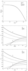 |
Fig. 1. Magnetic field strength and momentum dispersion in active region for model A. Panel a: Magnetic field strength in the active region versus height for model A. Panel b and c: Evolution of momentum dispersion β⊥ and β∥ of FEBs as precipitating along the flare loop with hight h = 5 × 10⁴ km and h = 1 × 10⁵ km according to model A. |
Figure 2a demonstrates the magnetic field behavior versus height h for model B. Figure 2b illustrates the evolution of momentum dispersion β⊥ and β∥ of FEBs when moving along the B-model flare loop. In this figure, the solid lines, dashed lines, and dot-dashed lines correspond to initial momentum dispersion β0 = 0.2c, β0 = 0.15c, and β0 = 0.1c, respectively. The height of the flare loop is set to h = 5 × 10⁴ km.
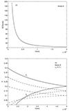 |
Fig. 2. Magnetic field strength and momentum dispersion in active region for model B. Panel a: Magnetic field strength in the active region versus height for model B. Panel b: Evolution of momentum dispersion β⊥ and β∥ of FEBs as precipitating along the flare loop according to model B. |
3. Numerical results
3.1. General formulation of the electron-cyclotron maser instability
The ECMI is a coherent mechanism that directly amplifies electromagnetic radiation, and it has been applied to various radio bursts. The first application of the ECMI was done by Wu & Lee (1979) to explain the Earth’s AKR. The essential physical feature that causes the instability is the relativistic effect in the cyclotron resonance condition. And electromagnetic waves can be amplified when the energetic electrons and waves meet the resonance condition:
 (6)
(6)
Here, γ denotes the Lorentz factor, while s represents the harmonic number. Parameters Ω and ωq denote the electron-cyclotron frequency and the frequency of the excited wave, respectively, with all frequencies normalized by the plasma frequency ωp. The terms Nq and θ denote the refractive index of the excited wave and the phase angle of the excited wave relative to the magnetic field, respectively. The subscript q indicates the wave mode, with q = + for the ordinary (O) mode and q = − for the extraordinary (X) mode.
According to the cold-plasma theory, the well-known dispersion relation is approximately given by (Wu et al. 2002; Chen et al. 2002):
 (7)
(7)
and
 (8)
(8)
When the frequency of the excited wave is ω ≃ sΩ, the temporal growth rate of the ECMI can be obtained with the following equation (Wu et al. 2002):
![Mathematical equation: $$ \begin{aligned} \omega _{\rm qi}\over \omega _{\rm ce}&= {\pi \over 2}{n_b\over n_0}\int \!\!\int \!\!\int d^3\mathbf{u}{\gamma \left(1-\mu ^2\right)\over \Omega \omega _q\left(1+T_q^2\right)R_q} \delta \left(\gamma -{s\Omega \over \omega _q}-{N_q\mu u\over c}\cos \theta \right) \nonumber \\&\quad \times \left\{ {\omega _q\over \Omega }\left[\gamma K_q\sin \theta +T_q\left(\gamma \cos \theta -{N_q\mu u\over c}\right)\right] {J_s(b_q)\over b_q}+J_s^\prime (b_q)\right\} ^2 \nonumber \\&\quad \times \left[u{\partial \over \partial u}+\left({N_qu\cos \theta \over c\gamma }-\mu \right){\partial \over \partial \mu }\right]F_b(u,\mu ), \end{aligned} $$](/articles/aa/full_html/2024/10/aa48081-23/aa48081-23-eq12.gif) (9)
(9)
here
 (10)
(10)
Here, nb and n0 represent the number densities of beam electrons and ambient thermal electrons, respectively. The term Js(bq) denotes the first kind of Bessel function.
3.2. Effect of temperature anisotropy on the electron-cyclotron maser instability
As mentioned in the previous subsection, the initial beam-like distribution will evolve into a temperature anisotropic distribution as FEBs travel down the flare loop. By utilizing Equations (2) and (3) along with the coronal magnetic field models of the flare loop, we can calculate the momentum dispersion β⊥ and β∥ of FEBs when electrons reach a certain height h. Figures 3–7 illustrate the effect of temperature anisotropy on the ECMI excited by the evolving FEBs as they propagate from the loop top to a certain height. For the given parameters (α, δ, uc, β0) of FEBs, the frequency ratio Ω, and the magnetic field model, we can calculate the growth rates of the ECMI when FEBs reach a certain height. The growth rate depends on the frequency and propagation angle of the excited wave (i.e., on parameters ωq and θ). Both the peak growth rate ωi and maximum growth rate ωmax are normalized by ωcenb/n0. Here, the steepness index δ = 6; spectrum index α = 3, uc = 0.3c; and frequency ratio Ω = 3.0 have been utilized.
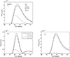 |
Fig. 3. Peak growth rates of the O1, O2, and X2 modes excited by the FEBs traveling down along the flare loop with a height of h = 5 × 10⁴ km. The parameters of FEBs, such as spectrum index α = 3; steepness index δ = 6, uc = 0.3c, and β0 = 0.5c; frequency ratio Ω = 3.0; and magnetic field model A have been used. |
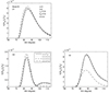 |
Fig. 4. Peak growth rates of the O1, O2, and X2 modes excited by the FEBs when traveling down along the flare loop. Here magnetic field model B has been employed, while other parameters remain the same as in Figure 3. |
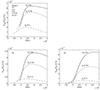 |
Fig. 5. Maximum growth rates of the O1, O2, and X2 modes excited by the FEBs traveling down along the flare loop with a height of h = 5 × 10⁴ km. The parameters of FEBs, such as spectrum index α = 3; steepness index δ = 6 and uc = 0.3c; frequency ratio Ω = 3.0; and magnetic field model A have been employed. The different curves correspond to different initial momentum dispersion β0. |
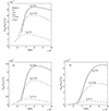 |
Fig. 6. Maximum growth rates of the O1, O2, and X2 modes excited by the FEBs traveling down along the flare loop with a height of h = 1 × 10⁵ km. The magnetic field model, parameters of FEBs, and frequency ratio remain consistent with those presented in Figure 5. |
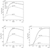 |
Fig. 7. Maximum growth rates of the O1, O2, and X2 modes excited by the FEBs traveling down along the flare loop with a height of h = 5 × 10⁴ km. The magnetic field model B has been used. The parameters of FEBs and the frequency ratio remain consistent with those presented in Figure 5. |
In Figure 3, Panels O1, O2, and X2 plot the peak growth rates of the fundamental waves of the O mode and the harmonic waves of the O and X modes, respectively. Here, the initial momentum dispersion is β0 = 0.2c, and the energetic electrons are accelerated at the top of a flare loop with a height h = 5 × 10⁴ km. The solid line in Figure 3 represents the peak growth rates of the ECMI excited by the FEBs when they just leave the acceleration region. The dotted line, dashed line, and dot-dashed line depict the growth rates of the ECMI when FEBs reach heights of h = 4.5 × 10⁴ km, h = 4.0 × 10⁴ km, and h = 3.0 × 10⁴ km, respectively.
We used the magnetic field model of the flare loop as model A, with parameters r, d, and B0 as in Figure 1a, to obtain the momentum dispersion β⊥ and β∥ for heights h = 4.5 × 10⁴ km, h = 4.0 × 10⁴ km, and h = 3.0 × 10⁴ km, respectively. As the FEBs travel down from the top of the loop to height h = 3.0 × 10⁴ km, we observed from Figure 3 that the peak growth rates of the ECMI do not change significantly as FEBs precipitate from the top of the flare loop to height h = 4.0 × 10⁴ km, but they notably decrease when FEBs reach height h = 3.0 × 10⁴ km. This trend suggests that the effect of temperature anisotropy on the ECMI is not significant at the beginning. From Figure 3, we note that the peak growth rates of the O1 mode and X2 mode are equivalent at the loop top, which is one order of magnitude higher than that of the O2 mode. This indicates that harmonic radiation exhibits anomalous mode polarization.
Figure 4 also displays the peak growth rates of the O1, O2, and X2 modes. In Figure 4, aside from the magnetic field model, the height of the flare loop, the parameters of the FEBs, and the frequency ratio are the same as in Figure 3. Using magnetic field model B and the initial momentum dispersion, we obtained the momentum dispersion β⊥ and β∥ from Equations (2) and (3) as FEBs reach heights h = 4.5 × 10⁴ km, h = 4.0 × 10⁴ km, and h = 3.0 × 10⁴ km, respectively. As depicted in Figure 4, the peak growth rates of the O1 and O2 modes exhibit a slight increase as FEBs move from the top of the loop to a height of h = 3.0 × 10⁴ km. However, the peak growth rates of the X2 mode remain virtually unchanged as the FEBs precipitate along the flare loop from the loop top to a height of h = 4.0 × 10⁴ km, and they then decrease by nearly half when FEBs reach a height of h = 3.0 × 10⁴ km. In Figures 2 and 4, it is evident that the growth rates reach their maximum values in directions that are close to perpendicular to the ambient magnetic field, displaying asymmetric profiles on either side of the maximum value. This implies that the radiation propagates quasi-vertically, and this asymmetry is generated by the anisotropy of the FEBs.
In Figures 5 and 6, we present the maximum growth rates of the O1, O2, and X2 modes as a function of height h. The heights of the flare loop are h = 5 × 10⁴ km and h = 1 × 10⁵ km for Figures 5 and 6, respectively. We used a spectrum index α = 3; a deepness index δ = 6, uc = 0.3c; a frequency ratio Ω = 3.0; and coronal magnetic field model A. The solid lines, dashed lines, and dot-dashed lines represent the maximum growth rates of the ECMI excited by the FEBs with initial momentum dispersion β0 = 0.2c, β0 = 0.15c, and β0 = 0.1c, respectively. The relationship between momentum dispersion and height h, shown in Figure 1b and 1c, results in variations of the maximum growth rates with height h in Figures 5 and 6. From these figures, it is evident that the maximum growth rates initially increase slowly and then decrease rapidly (for β0 = 0.2c, 0.15c) when the FEBs reach the critical height as they precipitate along the flare loop. For the X2 mode, the initial increase in growth rate is particularly slow, and it has a higher critical height. This explains why the peak growth rates of the O1, O2, and X2 modes in Figures 3 and 4 do not change much initially and then decrease rapidly, especially for the X2 mode. Figures 5 and 6 also show that the maximum growth rates of the O1 and X2 modes are comparable and approximately 20 times that of the O2 mode. This indicates that the harmonic radiation is X-mode polarized. Furthermore, Figures 5 and 6 illustrate that the maximum growth rates increase with the initial momentum dispersion β0. By comparing Figures 5 and 6, it is evident that the characteristics of the maser growth rates are independent of the height of the flare loop.
Figure 7 also depicts the maximum growth rates of the O1, O2, and X2 modes excited by FEBs descending along the flare loop with a height of h = 5 × 10⁴ km. The parameters of FEBs (α, δ, uc) and the frequency ratio parameter Ω remain consistent with those in Figure 5. Here, we used the magnetic field model of the flare loop as model B, and the solid lines, dashed lines, and dot-dashed lines correspond to the maximum maser growth rates of FEBs with an initial momentum dispersion of β0 = 0.2c, β0 = 0.15c, and β0 = 0.1c, respectively. Similar to Figures 5 and 6, the maximum growth rates exhibit a gradual increase followed by a sharp decline (for β0 = 0.2c, 0.15c) as FEBs precipitate along the flare loop. It also shows that the maximum growth rates of the O1 and X2 modes are one order of magnitude higher than that of the O2 mode. Comparing Figure 7 with Figure 5, it can be observed that the characteristics of the growth rate curve remain nearly unchanged. However, for magnetic field model B, the critical height at which the growth rate transitions from a slow rise to a rapid decline is lower. For instance, when the initial momentum dispersion is β0 = 0.2c, the critical height for model A is approximately 3.5 × 10⁴ km, whereas for model B, it is about 3.0 × 10⁴ km.
4. Summary and conclusions
The ECMI serves as a direct amplification mechanism for radio emissions occurring near the electron gyrofrequency and its harmonics within magnetized plasma. It is a crucial inherent mechanism and has been extensively applied to various radio phenomena, including auroral kilometer radiation on Earth as well as on other magnetized planets (Wu & Lee 1979) and short-duration solar radio bursts (Melrose & Dulk 1982).
It is widely recognized that various spatial anisotropic distributions of FEBs, such as loss-cone, ring-beam, and temperature anisotropy, contribute to the generation of free energy for the ECMI, particularly through the inversion of the perpendicular electron energy population. Temperature anisotropy is one of the most common anisotropic distributions observed in space plasma (Liu et al. 2007; Phillips et al. 1989; Gary et al. 2005). Melrose (1976)proposed that a temperature anisotropic distribution could arise when beam electrons precipitate along a magnetic field toward regions of increasing magnetic induction B. However, this model requires a notably high temperature anisotropy to efficiently excite the ECMI, largely due to non-relativistic resonance conditions. Tang et al. (2011)investigated maser emission excited by the lower energy cutoff behavior and temperature anisotropy of power-law electrons.
In this paper, we have explored the impact of temperature anisotropy, which arises as beam electrons travel downward along a flare loop, on the ECMI. These beam electrons are accelerated through magnetic reconnection processes during solar flares. Due to the conservation of the magnetic moment, the parallel energy of beam electrons is converted into perpendicular energy as they descend, resulting in a temperature anisotropic distribution. Our findings reveal that the temperature anisotropy generated during the descent of beam electrons significantly affects the ECMI. Specifically, as FEBs travel down along the flare loop, the calculations demonstrate that the maximum growth rates of the O1, O2, and X2 modes initially experience a slight increase, followed by a rapid decrease upon reaching a critical height for β0 = 0.2c and 0.15c. This indicates that the influence of temperature anisotropy on the ECMI becomes pronounced only after the FEBs reach the critical height.
The calculation results show that the growth rates of the O1 and X2 modes are comparable, about 20 times that of the O2 mode. This implies that the harmonic radiation is X-mode polarized. Usually, the X1 mode cannot escape directly, and it may undergo resonance mode conversion or nonlinear wave-wave coupling to become an escapable radiation wave. It deserves a completely separate investigation in the future.
In comparison to the O1 mode, the maximum growth rate of the X2 mode experiences a slower initial increase and exhibits a higher critical height. Additionally, our findings reveal that the maximum growth rates decrease with initial momentum dispersion β0, with the X2 mode showing a more rapid decline as β0 decreases. We used two magnetic field models to examine the evolution of the momentum dispersion and its impact on the ECMI as FEBs descend along the flare loop. Our results indicate that the temperature anisotropy induced by the motion of FEBs along the flare loops in the two different magnetic field models has similar effects on the ECMI. In this work, we do not account for the influence of a magnetic mirror on the distribution of FEBs, nor do we consider changes in the frequency ratio Ω at different heights. Therefore, more comprehensive research is warranted to explore these aspects.
Acknowledgments
This work is supported by the National Natural Science Foundation of China (NSFC) under grants 12173076 and 42174195, by Lishui University Initial Funding under grant QD2182, by National Key R&D Program of China 2021YFA1600503, as well as by the Strategic Priority Research Program of the Chinese Academy of Sciences under grant XDB0560000. Project Supported by the Specialized Research Fund for State Key Laboratories.
References
- Aschwanden, M. J. 1990a, A&AS, 85, 1141 [NASA ADS] [Google Scholar]
- Aschwanden, M. J. 1990b, A&A, 237, 512 [NASA ADS] [Google Scholar]
- Aschwanden, M. J. 2002, Space Sci. Rev., 101, 1 [Google Scholar]
- Aschwanden, M. J., & Benz, A. O. 1988, ApJ, 332, 466 [NASA ADS] [CrossRef] [Google Scholar]
- Bingham, R., Kellett, B. J., Cairns, R. A., et al. 2004, Contrib. Plasma Phys., 44, 382 [NASA ADS] [CrossRef] [Google Scholar]
- Camporeale, E., & Burgess, D. 2010, ApJ, 710, 1848 [NASA ADS] [CrossRef] [Google Scholar]
- Chen, Y. P., Zhou, G. C., Yoon, P. H., & Wu, C. S. 2002, Phys. Plasmas, 9, 2816 [NASA ADS] [CrossRef] [Google Scholar]
- Conway, A. J., & Willes, A. J. 2000, A&A, 355, 751 [NASA ADS] [Google Scholar]
- Dulk, G. A., & McLean, D. J. 1978, Sol. Phys., 57, 279 [CrossRef] [Google Scholar]
- Ergun, R. E., Carlson, C. W., McFadden, J. P., et al. 2000, ApJ, 538, 456 [NASA ADS] [CrossRef] [Google Scholar]
- Gary, S. P., Lavraud, B., Thomsen, M. F., Lefebvre, B., & Schwartz, S. J. 2005, Geophys. Res. Lett., 32, L13109 [NASA ADS] [CrossRef] [Google Scholar]
- Hess, S., Mottez, F., & Zarka, P. 2007, J. Geophys. Res.: Space Phys., 112, A11212 [NASA ADS] [Google Scholar]
- Hewitt, R. G., Melrose, D. B., & Ruennmark, K. G. 1981, PASA, 4, 221 [CrossRef] [Google Scholar]
- Liu, Y., Richardson, J. D., Belcher, J. W., & Kasper, J. C. 2007, ApJ, 659, L65 [NASA ADS] [CrossRef] [Google Scholar]
- Melrose, D. B. 1973, Aust. J. Phys., 26, 229 [NASA ADS] [CrossRef] [Google Scholar]
- Melrose, D. B. 1976, ApJ, 207, 651 [NASA ADS] [CrossRef] [Google Scholar]
- Melrose, D. B., & Dulk, G. A. 1982, ApJ, 259, 844 [Google Scholar]
- Melrose, D. B., & Wheatland, M. S. 2016, Sol. Phys., 291, 3637 [CrossRef] [Google Scholar]
- Phillips, J. L., Gosling, J. T., McComas, D. J., et al. 1989, J. Geophys. Res., 94, 6563 [NASA ADS] [CrossRef] [Google Scholar]
- Pick, M., & van den Oord, G. H. J. 1990, Sol. Phys., 130, 83 [NASA ADS] [CrossRef] [Google Scholar]
- Tang, J. F., & Wu, D. J. 2009, A&A, 493, 623 [NASA ADS] [CrossRef] [EDP Sciences] [Google Scholar]
- Tang, J. F., Wu, D. J., & Yan, Y. H. 2011, ApJ, 727, 70 [NASA ADS] [CrossRef] [Google Scholar]
- Tang, J. F., Wu, D. J., Chen, L., Zhao, G. Q., & Tan, C. M. 2016, ApJ, 823, 8 [NASA ADS] [CrossRef] [Google Scholar]
- Tang, J. F., Wu, D. J., Chen, L., Xu, L., & Tan, B. L. 2020, ApJ, 904, 1 [NASA ADS] [CrossRef] [Google Scholar]
- Tang, J. F., Wu, D. J., Chen, L., & Xu, L. 2023, Res. Astron. Astrophys., 23, 025009 [CrossRef] [Google Scholar]
- Treumann, R. A. 2006, A&ARv, 13, 229 [Google Scholar]
- Treumann, R. A., Nakamura, R., & Baumjohann, W. 2011, Geophys. Monogr. Ser., 29, 1673 [Google Scholar]
- Vlasov, V. G., Kuznetsov, A. A., & Altyntsev, A. T. 2002, A&A, 382, 1061 [NASA ADS] [CrossRef] [EDP Sciences] [Google Scholar]
- ŠtveráK, Trávníček, P., & Maksimovic, M. 2008, J. Geophys. Res.: Space Phys., 113, A03103 [Google Scholar]
- Wang, D.-Y. 2004, Chin. Astron. Astrophys., 28, 404 [Google Scholar]
- Wu, C. S., & Lee, L. C. 1979, ApJ, 230, 621 [Google Scholar]
- Wu, D. J., & Tang, J. F. 2008, ApJ, 677, L125 [NASA ADS] [CrossRef] [Google Scholar]
- Wu, C. S., Wang, C. B., Yoon, P. H., Zheng, H. N., & Wang, S. 2002, ApJ, 575, 1094 [NASA ADS] [CrossRef] [Google Scholar]
- Yoon, P. H., Wu, C. S., & Wang, C. B. 2002, ApJ, 576, 552 [NASA ADS] [CrossRef] [Google Scholar]
- Zarka, P., 1998, J. Geophys. Res., 103, 20159 [Google Scholar]
- Zhao, R.-Y. 1995, Ap&SS, 234, 125 [NASA ADS] [CrossRef] [Google Scholar]
- Zhao, G. Q., Chen, L., & Wu, D. J. 2013, ApJ, 779, 31 [NASA ADS] [CrossRef] [Google Scholar]
All Figures
|
Fig. 1. Magnetic field strength and momentum dispersion in active region for model A. Panel a: Magnetic field strength in the active region versus height for model A. Panel b and c: Evolution of momentum dispersion β⊥ and β∥ of FEBs as precipitating along the flare loop with hight h = 5 × 10⁴ km and h = 1 × 10⁵ km according to model A. |
| In the text | |
|
Fig. 2. Magnetic field strength and momentum dispersion in active region for model B. Panel a: Magnetic field strength in the active region versus height for model B. Panel b: Evolution of momentum dispersion β⊥ and β∥ of FEBs as precipitating along the flare loop according to model B. |
| In the text | |
|
Fig. 3. Peak growth rates of the O1, O2, and X2 modes excited by the FEBs traveling down along the flare loop with a height of h = 5 × 10⁴ km. The parameters of FEBs, such as spectrum index α = 3; steepness index δ = 6, uc = 0.3c, and β0 = 0.5c; frequency ratio Ω = 3.0; and magnetic field model A have been used. |
| In the text | |
|
Fig. 4. Peak growth rates of the O1, O2, and X2 modes excited by the FEBs when traveling down along the flare loop. Here magnetic field model B has been employed, while other parameters remain the same as in Figure 3. |
| In the text | |
|
Fig. 5. Maximum growth rates of the O1, O2, and X2 modes excited by the FEBs traveling down along the flare loop with a height of h = 5 × 10⁴ km. The parameters of FEBs, such as spectrum index α = 3; steepness index δ = 6 and uc = 0.3c; frequency ratio Ω = 3.0; and magnetic field model A have been employed. The different curves correspond to different initial momentum dispersion β0. |
| In the text | |
|
Fig. 6. Maximum growth rates of the O1, O2, and X2 modes excited by the FEBs traveling down along the flare loop with a height of h = 1 × 10⁵ km. The magnetic field model, parameters of FEBs, and frequency ratio remain consistent with those presented in Figure 5. |
| In the text | |
|
Fig. 7. Maximum growth rates of the O1, O2, and X2 modes excited by the FEBs traveling down along the flare loop with a height of h = 5 × 10⁴ km. The magnetic field model B has been used. The parameters of FEBs and the frequency ratio remain consistent with those presented in Figure 5. |
| In the text | |
Current usage metrics show cumulative count of Article Views (full-text article views including HTML views, PDF and ePub downloads, according to the available data) and Abstracts Views on Vision4Press platform.
Data correspond to usage on the plateform after 2015. The current usage metrics is available 48-96 hours after online publication and is updated daily on week days.
Initial download of the metrics may take a while.