| Issue |
A&A
Volume 680, December 2023
|
|
|---|---|---|
| Article Number | A61 | |
| Number of page(s) | 13 | |
| Section | The Sun and the Heliosphere | |
| DOI | https://doi.org/10.1051/0004-6361/202347414 | |
| Published online | 08 December 2023 | |
Dark halos around solar active regions
I. Emission properties of the dark halo around NOAA 12706
1
Università di Napoli “Federico II”, C.U. Monte Sant’Angelo, Via Cinthia, 80126 Naples, Italy
2
INAF – Osservatorio Astronomico di Capodimonte, Salita Moiariello 16, 80131 Naples, Italy
e-mail: This email address is being protected from spambots. You need JavaScript enabled to view it.
3
DAMTP, University of Cambridge, Wilberforce Rd, Cambridge, CB3 0WA, UK
Received:
10
July
2023
Accepted:
19
September
2023
Abstract
Context. Dark areas around active regions (ARs) were first observed in chromospheric lines more than a century ago and are now associated with the Hα fibril vortex around ARs. Nowadays, large areas surrounding ARs with reduced emission relative to the quiet Sun (QS) are also observed in spectral lines emitted in the transition region (TR) and the low corona. For example, they are clearly seen in the SDO/AIA 171 Å images. We name these chromospheric and TR-coronal dark regions “dark halos” (DHs). Coronal DHs are poorly studied and, because their origin is still unknown, to date it is not clear if they are related to the chromospheric fibrillar ones. Furthermore, they are often mistaken for coronal holes (CHs).
Aims. Our goal is to characterize the emission properties of a DH by combining, for the first time, chromospheric, TR, and coronal observations in order to provide observational constraints for future studies on the origin of DHs. This study also aims to investigate the different properties of DHs and CHs and provide a quick-look recipe to distinguish between them.
Methods. We studied the DH around AR NOAA 12706 and the southern CH that were on the disk on April 22, 2018 by analyzing IRIS full-disk mosaics and SDO/AIA filtergrams to evaluate their average intensities, normalized to the QS. In addition, we used the AIA images to derive the DH and CH emission measure (EM) and the IRIS Si IV 1393.7 Å line to estimate the nonthermal velocities of plasma in the TR. We also employed SDO/HMI magnetograms to study the average magnetic field strength inside the DH and the CH.
Results. Fibrils are observed all around the AR core in the chromospheric Mg II h&k IRIS mosaics, most clearly in the h3 and k3 features. The TR emission in the DH is much lower than in the QS area, unlike in the CH. Moreover, the DH is much more extended in the low corona than in the chromospheric Mg II h3 and k3 images. Finally, the intensities, EM, spectral profile, nonthermal velocity, and average magnetic field strength measurements clearly show that DHs and CHs exhibit different characteristics, and therefore should be considered as distinct types of structures on the Sun.
Key words: Sun: corona / Sun: atmosphere / Sun: chromosphere / Sun: transition region / Sun: activity / Sun: UV radiation
© The Authors 2023
 Open Access article, published by EDP Sciences, under the terms of the Creative Commons Attribution License (http://creativecommons.org/licenses/by/4.0), which permits unrestricted use, distribution, and reproduction in any medium, provided the original work is properly cited.
This article is published in open access under the Subscribe to Open model. This email address is being protected from spambots. You need JavaScript enabled to view it. to support open access publication.
1. Introduction
Active regions (ARs) on the Sun are typically surrounded by areas that in some wavelengths appear darker than the average quiet Sun (QS). They were first identified in the chromosphere as faint dark areas surrounding plages in theCa II K-line (Hale & Ellerman 1903; St. John 1911), and later also in the Ca II 8542 Å line (D’Azumbuja 1930). Deslanders (1930) called them “circumfacules”. Bumba & Howard (1965) found a spatial correlation between Ca II K-line circumfacules and the Hα fibril vortex around ARs and proposed that the Ca II circumfacular regions are composed of dark Hα fibrils. This suggestion was supported by many authors over the years (e.g., Veeder & Zirin 1970; Foukal 1971a,b; Harvey 2006; Rutten 2007; Cauzzi et al. 2008; Reardon et al. 2009; Pietarila et al. 2009).
Today, thanks to ultraviolet (UV) and extreme ultraviolet (EUV) observations, it is also possible to observe regions of reduced emission around ARs in a wide range of spectral lines originating in the transition region (TR) and the low corona. For instance, areas of reduced emission around ARs can be seen in the Solar Ultraviolet Measurements of Emitted Radiation (SUMER; Wilhelm et al. 1995) O V at 630 Å and S VI at 933 Å images1, as pointed out by Andretta & Del Zanna (2014). These authors referred to such structures as “dark halos” (DHs) as they were extended dark areas as seen in full-Sun SOHO/CDS TR lines. We adopt this name in this work from now on.
DHs are also clearly visible in the 171 Å images taken by the Atmospheric Imaging Assembly (AIA; Lemen et al. 2012) on board the Solar Dynamics Observatory (SDO; Pesnell et al. 2012), as noted by Wang et al. (2011), who instead named them “dark canopies”. These latter authors studied the relationship between the 171 Å DHs and the evolving photospheric field under the assumption that the 171 Å DH is the counterpart of the Hα fibrils. In other words, they assumed that it consists of EUV-absorbing chromospheric material (neutral hydrogen or helium) tracing out horizontal magnetic fields. However, as already pointed out by Andretta & Del Zanna (2014), inspection of DHs using SUMER observations reveals that these regions are seen darker even in lines at wavelengths longer than the edge of the Lyman continuum at 912 Å. Therefore, the interpretation based on absorption by neutral hydrogen cannot fully explain their low emission.
On the other hand, more recently, Singh et al. (2021) argued that the existence of DHs, which they call instead “dark moats,” is related to the magnetic pressure coming from the strong magnetic field that splays out from the AR, pressing down and flattening to a low altitude the underlying magnetic loops. These flattened loops, which would normally emit the bulk of the 171 Å emission, are restricted to heights above the surface that are too low to have 171 Å emitting plasma sustained in them, according to Antiochos & Noci (1986). According to this model, these loops are expected to have temperatures less than ∼5 × 10⁴ K. They should therefore emit into the emission passband of the 304 Å and appear bright in 304 Å images. However, DHs are generally visible as darker areas in 304 Å images by visual inspection, which means that this model is not entirely consistent with observations. Consequently, at the moment the physical mechanism responsible for the reduced emission of DHs remains poorly understood. Moreover, it is unclear whether the coronal EUV-observed DH is related to the chromospheric fibrillar one, as there are no previous studies analyzing them with chromospheric, TR, and coronal observations together. DHs are very common solar features, visible around ARs independently of the solar cycle and at all distances from the disk center, as shown for instance in Fig. 1. A DH could sometimes be mistaken for filament channels, which can frequently be observed in the Hα images (Makarov et al. 1982). We have verified that, for the ARs shown in Fig. 1 and for AR NOAA 12706 that we have studied in this work, no nearby filament channels are present in the Hα images (see Fig. A.1), and therefore these DHs are not filament channels.
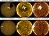 |
Fig. 1. From left to right: IRIS Mg II h core full-disk mosaic, AIA 171 Å and 193 Å images from April 13, 2019 (top panels) and May 5, 2019 (bottom panels), when the ARs NOAA 12738 and 12740, respectively, were on the disk. These two examples show the appearance of the DHs at the disk center and the solar limb, respectively. DHs are dark areas best seen in TR or low corona lines, such as Fe IX in the AIA 171 Å waveband. In the chromosphere, such as in Mg II h&k line cores, fibrils are often observed right next to the AR cores. |
DHs have a spatial extent comparable to that of the associated ARs, and therefore they may influence the irradiance of the Sun, especially during the maximum of solar activity when several ARs are present on the solar disk.
Furthermore, DHs are sometimes mistaken for coronal holes (CHs), and up to now there has not been a quantitative characterization that permits a clear distinction to be made between these two solar features. Andretta & Del Zanna (2014) note that these halos are easily seen in TR lines, while CHs are not. Singh et al. (2021) also observe that CHs tend to be dark across the six hotter AIA EUV wavelength passbands, in contrast with DHs, which are dark primarily in 171 Å but less so or not at all at other wavelengths such as 193 Å, as is also shown in Fig. 1.
Here we use a combination of imaging, spectroscopic, and magnetic field observations to comprehensively characterize the DH around AR NOAA 12706. This multiwavelength approach represents the first study of a DH through all the layers of the solar atmosphere, from the chromosphere up to the low corona. The aim of the work is to provide a quantitative characterization of the emission properties of a DH by using the Interface Region Imaging Spectrograph (IRIS; De Pontieu et al. 2014) full-disk mosaics and SDO/AIA (Lemen et al. 2012) images, in order to provide empirical constraints for the various hypotheses about the origin of DHs. In addition, our results show fundamental differences between the DH and the CH under study and support the thesis that DHs and CHs are two different types of structures on the Sun. At the end, we present a quick inspection method that can be used to distinguish a DH from a CH.
2. Observations
We selected AR NOAA 12706 for its suitable location on the disk in the IRIS mosaics: its intermediate position between the limb and the disk center makes it possible to look under the coronal loops when looking at AIA images. AR NOAA 12706 displays a β magnetic configuration characterized by one sunspot of negative polarity and a more diffuse positive magnetic concentration as little dark pores. It was visible on the disk from April 20 to April 28, 2018. On April 20, a “light bridge” (see e.g., van Driel-Gesztelyi & Green 2015; Falco et al. 2016; Felipe et al. 2016 and reference therein) begins to form within the negative polarity sunspot, indicating the onset of its fragmentation. Indeed, the spot completely vanishes on April 27. This AR was observed in a temporal interval of ∼4 h by IRIS on April 22, 2018 during the full-disk observation mode, which started on April 22 at 10:41:50 UT and finished on April 23 at 04:05:45 UT. Southwest of NOAA 12706 is NOAA 12707, a smaller, decaying AR that disappears from the disk after about two days. Given its small size, we assume that its presence does not influence the area around AR 12706, and therefore we do not include it in the analysis. The same IRIS Mg II mosaics have been studied previously by Bryans et al. (2020) and the AR NOAA 12706 is one of the seven ARs studied by Singh et al. (2021). We discuss our results in relation to those of these authors in Sect. 5.
2.1. IRIS full-disk mosaics
Primarily used for quasi-regular monitoring of changes in instrument sensitivity, IRIS full-disk mosaics have proven to be very useful in the study of the solar atmosphere, as they have been employed in a variety of ways (see e.g., Schmit et al. 2015; Vial et al. 2019; Bryans et al. 2020; Ayres et al. 2021; Koza et al. 2022). IRIS full-disk mosaics consist of spectral maps of the entire solar disk built through an observing sequence (currently run approximately once per month, when IRIS is not in eclipse season) that takes a series of successive rasters at 184 different pointing locations. Rasters’ spectral windows include the six strongest spectral lines, the resonance lines Mg II h&k (T ∼ 8 × 10³ K), C II 1335 and 1334 Å (∼104 K), and Si IV 1393 and 1403 Å (∼6 × 10⁴ K). All 184 positions take ∼18 h, including ∼10 h of time taken to repoint the spacecraft (Schmit et al. 2015). Each individual observation consists of a 64-step raster with 2″ steps and 2 s exposure time at each slit position. The spectra along the slit have been binned to a resolution of 0.33″. Mg II mosaics have a spectral scale of 35 mÅ px−1, while C II and Si IV have a spectral scale of 25 mÅ px−1. Thus, the spectral range of 3.5 Å for Mg II lines and of 1 Å for C II and Si IV lines is sampled by 101 and 41 spectral points, respectively.
For this work, mosaics represent a unique resource with which to investigate the morphological features of DHs, which have a spatial extent comparable to that of the associated ARs and which could not be properly studied through normal rasters, given their usually relatively small field of view (FoV). In addition, the available spectral windows allow a view of both the chromosphere and the TR, thanks to the chromospheric Mg II h&k lines and the C II and Si IV TR doublets.
2.2. SDO data
In order to characterize the emission properties of the DH in the corona, we used AIA observations for their full-Sun coverage. DHs are relatively stable structures that evolve in timescales on the order of the AR evolution time (∼days, see e.g., van Driel-Gesztelyi & Green 2015). Therefore, rather than analysing all the AIA images in the four-hour period taken by IRIS to entirely cover the AR by rasters, we studied only the AIA image taken at 19:24 UT, which is approximately in the middle of the ∼4 h temporal window.
To study the evolution of the magnetic flux along the line of sight, we also used a series of Helioseismic and Magnetic Imager (HMI; Schou et al. 2012) LOS magnetograms taken in the Fe I 617.3 nm line with a resolution of 1″. They cover ∼30 min of observations, from 19:07:30 UT to 19:36:45 UT, with a cadence of 45 s.
3. Analysis
To quantitatively characterize the emission properties of the DH in the different layers of the solar atmosphere and compare them to the QS and the CH properties, we defined four regions of interest (RoIs), described below. For the DH, the starting point of the analysis is the annular region, the emission of which is reduced compared to the QS seen by eye in the IRIS Mg II h&k core full-disk mosaics (e.g., see the left panel of Fig. 2 and the top panel of Fig. 4). In particular, fibrils are clearly observed in the Mg II h&k cores (i.e., the 50th spectral point for both lines; see the right panel of Fig. B.1). Fibrils are chromospheric features visible mainly in nearline-core wavelengths of the chromospheric lines (see e.g., Kianfar et al. 2020). Indeed, in IRIS Mg II mosaics it is also possible to notice that they become less visible as the selected wavelength approaches the line wings, where they become fainter and eventually undetectable (see Fig. B.1), meaning that they are upper chromospheric features.
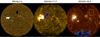 |
Fig. 2. IRIS Mg II h3 full-disk mosaic and AIA full-disk images showing the DH surrounding AR NOAA 12706 in the northern hemisphere on April 22, 2018. The three images are center-to-limb corrected. Left panel: the three fibrillar DH contours are shown in shades of green and the outer AR-core edge is shown in red. Middle and right panels: AIA 171 and 193 Å filtergrams, respectively, taken at 19:24 UT. The three coronal DH contours are shown in shades of violet in the AIA 171 Å image, while the QS box and the three southern CH contours are shown in white and in shades of blue, respectively, in the AIA 193 Å image, as described in Sect. 3. The contours are obtained through intensity thresholds from the non center-to-limb corrected images. |
Because the fibrils around the AR are most visible at the Mg II h&k cores, we only used the h3 and k3 images2 in our analysis, found through a double Gaussian fit of the Mg II h&k lines. We used the defroi.pro IDL routine to manually draw, in the Mg II h3 mosaic, the outer boundary of the DH, visually following the fibrils, and the outer edge of the AR core that is the inner DH contour. These two contours are shown in the left panel of Fig. 2 in green and red, respectively. We refer to the DH identified by these two contours as a “chromospheric fibrillar DH”. We point out that the close NOAA 12707, on the contrary, does not exhibit a chromospheric DH made up of fibrils extending radially from the AR core, but does have a few dark filamentous structures surrounding it.
Looking at AIA filtergrams (see Fig. 5), we noticed that the DH is most visible in the AIA 171 Å image, as is also shown by Wang et al. (2011) and Singh et al. (2021). In this waveband, the DH spatial extent is larger than in the Mg II mosaics, with coronal loops in the immediate vicinity of the AR core partially covering and hiding the dark emission beneath them. Therefore, we decided to use a second contour for the coronal 171 Å DH, which we call a “coronal DH”, located on the west side of the AR. We defined it through an intensity threshold equal to 55% of the 171 Å average disk emission. We used this particular value because the area falling inside the corresponding contour is close to the dark region identifiable by eye. This new contour, used to evaluate the average intensity of the coronal DH, is shown in violet in the middle panel of Fig. 2. We point out that, in this image, projection effects prevent the east side of the coronal DH from being visible; it is instead well observed following the AR during its transit on the solar disk.
For the CH definition, we used another intensity threshold, equal to 35% of the 193 Å average disk emission. Tools based on the intensity threshold of coronal EUV images have been widely used for the detection of CHs in the past (e.g., Krista & Gallagher 2009; Reiss et al. 2015; Heinemann et al. 2019). The CH contour is shown in blue in Fig. 2. For the QS we used a box of 250″ × 337″ located outside the CH and AR areas (see the right panel in Fig. 2) and chosen such that its radial distance from the center is approximately similar to that of the AR, in order to minimize center-to-limb variations. In summary, we have defined four RoIs, shown in Fig. 2:
-
a chromospheric fibrillar DH;
-
an upper coronal DH;
-
a southern CH;
-
a QS.
3.1. Data processing
The AIA images were processed by first deconvolving the psf with the IDL routine aia_deconvolve_richardsonlucy.pro. All IRIS mosaics were first of all processed using the new_spike.pro IDL routine in order to remove spikes. In the C II and Si IV mosaics an anomalous background was present and was thought to be a calibration issue, likely related to incomplete compensation for stray light contamination (see Ayres et al. 2021 for further details). For this reason a background was calculated and subtracted, as was also done by Ayres et al. (2021). In particular, for every spatial pixel, we evaluated the background, Ibkg, as follows:
 (1)
(1)
where ired ∈ [λref + 12Δλ, λref + 19Δλ], iblue ∈ [λref − 19Δλ, λref − 12Δλ], and where λref represents the QS reference wavelength and Δλ = 0.025 Å corresponds to the spectral scale of C II and Si IV. The C II and Si IV background spectral intervals are shown as gray bands in Fig. 3.
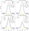 |
Fig. 3. C II 1334 and 1335 Å (upper panels) and Si IV 1393 and 1403 Å (lower panels) average profiles for QS, fibrillar and coronal DH and CH, in red, green, violet, and cyan respectively, with corresponding normalized histograms of the integrated intensities. The vertical dotted lines in the profiles represent the QS reference wavelengths. The yellow and gray bands identify the spectral intervals used for C II and Si IV intensity and background evaluation, respectively. In the lower left panels, the dashed curves are the Si IV 1393 Å fits. |
We then corrected the line intensities for the center-to-limb variation, as described in the appendix. In Fig. 3 we show the center-to-limb corrected average line profiles for C II and Si IV doublets inside the four RoIs, that is, the QS, the fibrillar DH, the coronal DH, and the CH, with the corresponding normalized histograms of the integrated intensities.
For C II and Si IV, we used the mosaics after the above processing computed integrating the lines on the spectral intervals shown as yellow bands in Fig. 3. In Fig. 4 we show a closeup view of AR NOAA 12706 as observed, from top to bottom, in Mg II h3 and in the background-removed and peak-integrated Si IV 1393 Å and C II 1334 Å center-to-limb corrected mosaics. These zooms are representative also of Mg II k3, Si IV 1403 Å, and C II 1335 Å, respectively, which we do not show because they appear remarkably similar.
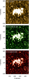 |
Fig. 4. Closeup view of NOAA 12706 and its surroundings. From top to bottom: IRIS Mg II h3, Si IV 1393 Å, and C II 1334 Å. North is up and west is to the right. The FoV has dimensions 440″ × 410″. In the Mg II h3 it is possible to observe around the AR core the chromospheric DH made up of fibrils that have a maximum length approximately half the size of the AR in the longitudinal direction. In the C II and Si IV mosaics, instead, a halo of reduced emission is still recognizable around the AR, but less clearly and without the evident presence of fibrillar structures. |
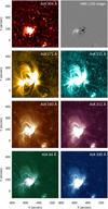 |
Fig. 5. AIA closeup views of NOAA 12706 and its surroundings. North is up and west is to the right. The FoV has dimensions 700″ × 620″. |
3.2. Average intensity measurements
In order to quantitatively characterize the emission properties of the fibrillar and coronal DHs, we evaluated the average intensity (in DN) inside the four RoIs. We applied the contours defined before as follows:
-
the annular Mg II h3 fibrillar DH contour was applied to all IRIS mosaics;
-
the AIA 171 Å coronal DH contour was applied to all AIA filtergrams;
-
the same AIA 193 Å CH contour was applied to all IRIS mosaics and AIA filtergrams;
-
the same QS box was applied to all IRIS mosaics and AIA filtergrams.
Then we normalized the fibrillar DH, the coronal DH, and the CH average intensities to the QS by computing the ratio defined as
 (2)
(2)
where the RoIs are the fibrillar DH, the coronal DH, and the CH.
The uncertainties of the ratios defined in the above Eq. (2) are in principle the result of the propagation of the uncertainties attached to each step of the analysis, which are the definition of the RoI, the calculation of the average intensity within the RoI, and the center-to-limb correction. In the case of intensities from IRIS spectra, we considered in addition the uncertainty due to the definition of the spectral intervals used for evaluating the background and the total intensity, and the contribution from the noise in each spectral pixel of the profile. We evaluated each one of these sources of uncertainty and found that by far the largest contribution is due to the RoI selection criteria.
In order to estimate the uncertainties of the ratio given by Eq. (2), we then proceeded as follows:
-
For the fibrillar DH, we drew by hand two additional contours by being more and less restricted on the fibril-edge definition. These contours are shown in different shades of green in the left panel of Fig. 2;
-
For the coronal DH and CH, we changed the value of the intensity thresholds defining the RoIs; in particular, we considered a 2% variation in the thresholds defining the coronal DH RoI; in other words, we considered two additional contours at 55% and 59% of the mean disk value, and a 10% variation for the CH RoI, at 25% and 45% of the mean disk value. We thus obtained, for each of those RoI, two additional regions slightly smaller and larger, respectively, than the reference RoI. The resulting three coronal DH contours are shown in violet in the middle panel of Fig. 2; the three CH contours are shown in blue in the right panel of Fig. 2.
The uncertainties of the ratios of Eq. (2) were then obtained by computing the difference of the mean intensities in these additional regions with respect to the value obtained in the reference RoI.
The ratios of the selected RoIs, and the associated uncertainties computed as described above, are shown in Fig. 6. The dispersion of the ratios shown with shaded green and blue bands was obtained by using additional contours of a slightly different extent to give an estimate of the ratio variability. These results are discussed in more detail in Sect. 4.
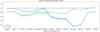 |
Fig. 6. DH (in green) and southern CH (in blue) average intensity ratios in IRIS lines and AIA filters. The shaded areas are the ratio uncertainties, computed as discussed in Sect. 3. The chromospheric fibrillar and the 171 Å coronal DH contours were employed for the IRIS and AIA ratios, respectively. |
3.3. Nonthermal velocity measurements
In the TR the profiles of the spectral lines often exhibit, in addition to the thermal and instrumental broadenings, excess broadening that is associated with unresolved plasma motions that can transfer mass and energy between the chromosphere and the corona. These plasma flows are likely to be intimately related to the still unknown physical processes occurring in the TR. We studied the nonthermal broadenings inside the four defined RoIs using the optically thin line, Si IV 1393.7 Å. For optically thin lines the spectral profile is assumed to be Gaussian and the Gaussian width, σ, can be expressed as (Del Zanna & Mason 2018)
 (3)
(3)
where c, k, Ti, σI, ξ are, respectively, the speed of light, the Boltzmann constant, the temperature of the ion, the additional instrumental broadening, which is 3.9 km s−1 for IRIS (Del Zanna & Mason 2018; De Pontieu et al. 2014), and the nonthermal velocity, which represents the most probable velocity of the random plasma motions.
We estimated σ inside the QS, the fibrillar DH, the coronal DH, and the CH by fitting the Si IV 1393 Å mean line profiles shown in Fig. 3 with a Gaussian and a constant term. We assumed a Si IV formation temperature of 60 × 103 K. This is lower than the temperature of 80 × 103 K obtained in CHIANTI using the zero-density ionization equilibrium (Dere et al. 2019), and was derived with the new ionization equilibrium calculations of Dufresne et al. 2021 that include density-dependent effects and charge transfer. The fits for the four RoIs are shown in the bottom left panel of Fig. 3. The fit parameters and nonthermal velocities, ξ, found are reported in Table 1. The fit parameters, I0, λ0, I1, and σ, are the height, the center, the constant term, and the standard deviation of the Gaussian, respectively.
Si IV 1393 Å Gaussian fit parameters inside the fibrillar DH, the coronal DH, the CH, and the QS.
3.4. Emission measure
To deduce the temperature distribution of the coronal plasma along the LOS from the AIA filtergrams, we calculated inside the coronal DH, the QS, and the CH the average total column emission measure function, EM, defined as
![Mathematical equation: $$ \begin{aligned} \mathrm{EM}=\int _h N_{\rm e}^2 \mathrm{d}h= \int _T \mathrm{DEM}(T) \mathrm{d}T,\quad \quad \quad \quad [\mathrm{cm}^{-5}] \end{aligned} $$](/articles/aa/full_html/2023/12/aa47414-23/aa47414-23-eq4.gif) (4)
(4)
where Ne is the electron number density and DEM(T) is the column differential emission measure, defined as  .
.
We calculated the DEM(T) function by employing the sparse inversion technique of Cheung et al. (2015), which assumes that the intensity in each pixel of an image from the jth AIA waveband can be written as
 (5)
(5)
where Kj(T) is the function that describes the response of the jth channel with the temperature. This method inverts the previous equation obtaining DEM solutions after giving as input the EUV images from the AIA channels 94, 131, 171, 193, 211, and 335 Å and the temperature response functions of these channels. We implemented this technique through the routines aia_sparse_em_init.pro and aia_sparse_em_solve.pro, available in IDL SolarSoft. The first one builds up the response functions, while the second one is the proper DEM solver.
We then obtained the average emission measures using Eq. (4) by integrating the DEM over the temperature range from log T[K]=5.6 to log T[K]=6.3. We did not evaluate the average emission measure inside the fibrillar DH because AR loops cover that RoI.
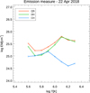 |
Fig. 7. Average log EM curves as functions of log T calculated over the QS, coronal DH, and southern CH. The DH and the CH show a similar depletion in EM compared to the QS in the 5.6–5.9 log T range. At higher temperatures the CH exhibits a trend opposite to that of DH and QS, with a strong EM reduction. |
3.5. HMI magnetic field strengths
We used the time series of HMI magnetograms to investigate the temporal evolution of the average signed, ⟨BLOS⟩, and unsigned, ⟨|BLOS|⟩, magnetic field strength inside the four RoIs. The noise level of 45-s magnetograms exhibits a center-to-limb variation, being lower near the disk center and increasing radially approaching the limb up to ∼8 G (Yeo et al. 2013). Therefore, we cut all the pixels in the range [−8,8] G. The results of the average signed and unsigned magnetic field strength measurements, together with the standard deviations, are reported in Fig. 8. We point out that the magnetic field strength depends on the threshold used in the noise removal. However, we find that the relative distances between the RoIs also remain the same when using different thresholds.
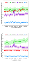 |
Fig. 8. Average signed (top panel) and unsigned (bottom panel) magnetic field strength ∼30 min time evolution inside the four RoIs. The colored bands are the uncertainties. |
4. Results
The first results we show are the C II 1334 and 1335 Å (upper panels) and Si IV 1393 and 1403 Å (bottom panels) mean line profiles of Fig. 3. The QS, fibrillar DH, coronal DH, and CH profiles are shown in red, green, violet, and cyan, respectively, after the background removal and the center-to-limb correction. The Gaussian Si IV fits are added in the bottom panels of Fig. 3. At the same time, we show the histograms of the integrated intensity (in DN) inside the RoIs, normalized to the number of spatial pixels. We do not show the Mg II profiles because in the analysis we use only the h3 and k3 images.
The Si IV lines have Gaussian profiles, while the C II lines are flatter than a Gaussian, as also reported in Upendran & Tripathi (2021) for the CH and QS cases. We also notice a hinted double peak in the C II CH line. In all cases, the DH presents narrower lines and slightly higher intensity peaks than the CH (except for the Si IV 1403 Å line). In the four lines the QS is more intense than the other RoIs, with the only exception being the coronal DH, which is nearly identical to the QS in the C II lines. Overall, we do not find evident Doppler shifts in the profiles.
The histogram shapes are unimodal and have a broader right side, probably due to bright points. The four lines display a similar histogram for the intensities scheme: the DH distribution (green) is shifted toward smaller intensity counts and has a peak value between those of the QS and the CH.
Regarding the nonthermal velocities obtained with the Gaussian Si IV 1393 Å fit, the results of which are shown in Table 1, we find that the plasma has nonthermal velocities ξ of ∼22, 26, 26, and 28 km s−1 inside the fibrillar DH, coronal DH, QS, and CH, respectively, with the coronal DH having essentially the same ξ as the QS. The QS value is close to the averaged values found by Rao et al. (2022).
In Fig. 6 we show the DH (in green) and CH (in blue) ratios for the IRIS lines and the AIA bands. The IRIS lines are sorted according to the nominal formation temperature, as determined from the standard CHIANTI ionization equilibrium. The IRIS and AIA DH ratios are referred to the fibrillar and the coronal DH, respectively. A fibrillar DH is observed in all IRIS lines, because IRIS ratios are less than one, and it is darkest in the C II lines. The CH ratios display a similar trend but with higher ratios, closer to one. In the AIA side of the plot, the coronal DH shows ratios less than one in all filters, except for the AIA 94 Å with a positive trend increasing with temperature. On the other side, the CH shows evidence of different behavior: the CH has a drop in intensity relative to the QS, which reaches a minimum in the AIA 193 and 211 Å bands and then increases in the hottest AIA bands. Therefore, the fibrillar and coronal DHs show approximately constant ratios on the order of 0.8, which increase when approaching the hottest AIA bands. On the contrary, the CH exhibits the opposite behavior, being almost invisible in the chromosphere and TR and becoming evident when approaching the corona.
Figure 7 shows the average EM as a function of temperature obtained using the AIA filtergrams for the QS, the coronal DH, and the CH in red, green, and cyan, respectively. The plot shows clearly that in the temperature range log T[K]=5.6 − 6.1 both the coronal DH and the CH have a lower emission measure than the QS, while in the range log T[K]=6.1 − 6.3, corresponding to the AIA channels 193 and 211 Å, the DH and the CH again exhibit the opposite behavior. We note that the DH and QS emission measure results in the temperature range log T[K]=5.6 − 6.3 are comparable with those found by Singh et al. (2021), even if the RoIs are selected differently and the center-to-limb effect is not corrected.
In Fig. 8 we plot the average signed and unsigned magnetic field strength in the four RoIs obtained from the ∼30-min sequence of magnetograms. We find that during the selected time interval the magnetic field strengths remain constant and only the fibrillar DH displays a weak time evolution, probably related to new flux emerging in the RoI. We find that the fibrillar DH and the QS have similar averaged signed magnetic fields strengths, close to zero (consistent with the results by Wang et al. 2011), while the CH is unipolar, and the coronal DH presents values intermediate between the CH and the QS. On the other side, the fibrillar and coronal DHs show average unsigned magnetic field strengths higher than the QS, and the CH displays the lowest values.
In Fig. 9 we also show the 30-min averaged QS-subtracted normalized histograms, which were obtained by first normalizing the 30-min averaged histograms to the total number of pixels and then subtracting the QS histogram. We find that the fibrillar and coronal DH histograms are centered on the zero, while the CH histogram peak is shifted toward negative magnetic field strength values.
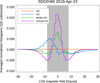 |
Fig. 9. Averaged QS-subtracted histograms of the four RoIs. The gray band corresponds to the noise interval, [−8,8] G, that was cut to obtain the magnetic field strength measurements shown in Fig. 8. |
5. Discussion and conclusions
Dark halos have for a long time been observed as “circumfacular regions” surrounding ARs, but have also been known under different names. Typically, they appear as regions darker than the QS in chromospheric or TR lines. These large-scale structures are normally best studied in full-Sun imaging or imaging spectroscopy. We thus inspected the available set of IRIS full-Sun mosaics (2013 to present) and found that most ARs’ surroundings exhibit clear DH signatures in the core of the Mg II h & k lines, appearing as dark fibrils with almost radial symmetry around the AR core. We therefore concluded that these structures are very common solar features. Nevertheless, the literature describing these structures is very sparse, providing only a partial view in one or two wavelengths only.
In this work, we present the first quantitative characterization of the emission properties of the DH associated with AR NOAA 12706, from the chromosphere to the low corona, using IRIS full-Sun mosaics and SDO/AIA images. We complement the results with a preliminary analysis of the SDO/HMI magnetograms.
We find that IRIS scans in the C II and Si IV lines of the area around NOAA 12706 show that the DH seen in those lines coincides with the region covered by Mg II fibrils, although no clear fibrillar pattern could be detected in those TR lines.
Extending the analysis to SDO/AIA images confirms that DHs are clearly visible in the 171 Å band, as already noted by other authors (Wang et al. 2011; Singh et al. 2021). However, we also find that the area of the AIA 171 Å DH seems to be significantly larger than in IRIS chromospheric and TR lines, although a direct comparison over the entire region is difficult due to the presence of bright AR loops in the line of sight in many places. In this work we therefore distinguish between the DH seen in Mg II h & k line core and in AIA 171 Å, which we term “fibrillar” and “coronal” DHs, respectively. It is not yet clear if and how the two structures are related, but it seems plausible that the “coronal” DH encompasses and extends the “fibrillar” DH. This point clearly deserves further investigation, which we are currently carrying out, by analysing for instance a larger set of ARs over a larger range of wavelengths than in the current study.
In this context, it might be worth noting that the AIA 304 Å line seems to share traits of both kinds of DHs: filtergrams at that wavelength are clearly darker in the fibrillar DH, but the extended area corresponding to the coronal DH is also noticeably darker than the average QS.
DHs are a clear feature in TR lines. Andretta and Del Zanna note their presence around all ARs in TR lines observed by the SOHO/CDS and SOHO/SUMER full-disk scans. Our analysis, in effect, shows that fibrillar DHs are clearly detectable in TR lines, in particular above the Lyman continuum edge; it is therefore unlikely that the appearance of these structures could be due to absorption by cool material, as postulated by Wang et al. (2011). However, the IRIS C II and Si IV lines are formed at temperatures low enough that the coronal DH, observed clearly in the AIA 171 Å band, is not visible.
Considering that DHs seen in the AIA 171 Å waveband appear remarkably similar to coronal holes (CHs), we also compared in detail the properties of those two structures, comparing in particular both the “fibrillar” and “coronal” with the CH seen on the same date at the south pole, using as reference a patch of QS. Our analysis took into account the effect of average center-to-limb variation, which is quite apparent in the intensities of most lines and wavebands in the dataset.
In addition, we computed average values of the signed and unsigned magnetic field in the regions under studies, using SDO/HMI data taken during the same interval as the IRIS raster scans covering the selected regions.
Our analysis clearly indicates that the DH and the CH under study are different structures, as summarized by the following results:
-
fibrils seen in Mg II h & k line core are found only in the area around the associated AR, in other words in the fibrillar DH;
-
compared to the reference QS area, the line intensities are different over a wide range of temperatures, a finding that is confirmed by analysis of the emission measures;
-
the average C II and Si IV line profiles in the two regions are different, with the Si IV lines in particular exhibiting slightly different nonthermal widths compared to both the QS and CH;
-
both the fibrillar and coronal DHs on average do not appear to be as markedly unipolar as the CH;
-
the average signed magnetic field in the fibrillar DH, in particular, seems to be vanishingly small, as in the reference QS patch.
We speculate that the above results are valid for all ARs. If this is the case, some of the differences between DHs and CHs could provide proxies for distinguishing the two structures. Such proxies could be especially useful in the case of CHs close to ARs, for example in the case of equatorial CHs.
In particular, we propose that the different DH and CH emission characteristics in the AIA filters can be used as a simple recipe to distinguish between DHs and CHs. More specifically, as illustrated by Figs. 5 and 6, DHs are clearly outlined in the AIA 171 Å waveband, while they are nearly indistinguishable from quiescent coronal areas in the AIA 193 Å or AIA 211 Å wavebands. On the contrary, CHs are dark in all AIA coronal bands, including AIA 193 Å or AIA 211 Å.
An illustrative example of the above recipe is given by the cases of ARs NOAA 12738 and 12740 shown in Fig. 1, which display a β and an α3 configuration, respectively. In both cases, fibrils are observed around the brightest part of the AR in the Mg II h & h line core. The DH is also clearly detectable around both ARs in the AIA 171 Å images. On the contrary, the AIA 193 Å filtergrams do not show any significantly darker area around the AR cores. The CH is instead well visible in both the AIA 193 and 171 Å wavebands.
IRIS mosaics are taken only once per month. This means that it is not always possible to check for the presence of fibrils around an AR. However, we highlight that the AIA 304 Å channel, given its peculiarity of showing the annular shadow of fibrils around the AR cores, can be used to provide an estimate of the spatial location of the fibrillar DH in the chromosphere when IRIS data are not available.
DHs are large-scale, long-lasting structures that are clearly associated with ARs. While they apparently persist and perhaps evolve throughout the AR lifetime, they are most likely related to the AR emergence process. There is clearly much less TR plasma connecting the opposite polarities compared to QS regions. The causes could be related to a different magnetic flux emergence in DHs that leads to a different coronal heating compared to the QS areas, or to processes occurring in the corona (or both). Regarding the latter, it is worth mentioning that dark regions were found around a few isolated ARs studied by Del Zanna et al. (2011). They were, on large scales, relatively unipolar, which led the authors to propose an interchange reconnection model between these regions and the hot AR core loops. It is clear that some interaction must occur between the emerging flux in the cores of ARs and the surrounding preexisting corona, but it is unclear if the DHs are related to the interchange reconnection process, especially if it is confirmed that, in terms of magnetic field configurations, they are QS-like regions of largely mixed polarity.
In conclusion, DHs remain remarkably common, large, and persistent solar structures, and yet their characteristics and nature are largely unknown. With this work we have begun to provide a first characterization of the emission properties of such structures. We are carrying out follow-up studies to better determine the properties of these features. They include the use of Hinode/EIS (Culhane et al. 2007) spectroscopic data to better characterize the changes in the TR-coronal emission, and of Solar Orbiter EUI images (Rochus et al. 2020) to study DHs at a much higher spatial resolution than AIA. We are also carrying out an analysis of the evolution of DHs in terms of TR-coronal properties and the photospheric magnetic field.
See, for instance, the June 7, 1996 and May 12, 1996 images on SUMER atlas at https://ads.harvard.edu/books/2003isua.book/.
We use the well-known nomenclature to define h3 as the central depression of the line, h2r as the red emission peak and the h1r as the minimum on the red side of the central emission peak. These positions are shown as example in the Mg II h full-disk mean profile of Fig. B.1 (right panel).
An AR containing a single sunspot or group of sunspots all having the same magnetic polarity.
Acknowledgments
This study was partly supported by the Italian agreement ASI-INAF 2021-12-HH.0 “Missione Solar-C EUVST – Supporto scientifico di Fase B/C/D”. GDZ acknowledges financial support from STFC (UK) via the consolidated grants to the atomic astrophysics group (AAG) at DAMTP, University of Cambridge (ST/T000481/1 and ST/X001059/1). The authors acknowledge important suggestions from the anonymous referee who helped to improve the manuscript. This study has made use of SAO/NASA Astrophysics Data System’s bibliographic services. IRIS is a NASA small-explorer mission developed and operated by LMSAL with mission operations executed at the NASA Ames Research Center and major contributions to downlink communications funded by the European Space Agency and the Norwegian Space Center. CHIANTI is a collaborative project involving George Mason University, the University of Michigan (USA), University of Cambridge (UK) and NASA Goddard Space Flight Center (USA).
References
- Andretta, V., & Del Zanna, G. 2014, A&A, 563, A26 [NASA ADS] [CrossRef] [EDP Sciences] [Google Scholar]
- Antiochos, S. K., & Noci, G. 1986, ApJ, 301, 440 [CrossRef] [Google Scholar]
- Ayres, T., De Pontieu, B., & Testa, P. 2021, ApJ, 916, 36 [NASA ADS] [CrossRef] [Google Scholar]
- Bumba, V., & Howard, R. 1965, ApJ, 141, 1492 [CrossRef] [Google Scholar]
- Bryans, P., McIntosh, S. W., De Moortel, I., & De Pontieu, B. 2020, ApJ, 905, L33 [NASA ADS] [CrossRef] [Google Scholar]
- Carella, F., & Bemporad, A. 2020, INAF Technical Report, http://hdl.handle.net/20.500.12386/26079 [Google Scholar]
- Cauzzi, G., Reardon, K. P., Uitenbroek, H., et al. 2008, A&A, 480, 515 [NASA ADS] [CrossRef] [EDP Sciences] [Google Scholar]
- Cheung, M. C. M., Boerner, P., Schrijver, C. J., et al. 2015, ApJ, 807, 143 [Google Scholar]
- Culhane, J. L., Harra, L. K., James, A. M., et al. 2007, SoPh, 243, 19 [NASA ADS] [Google Scholar]
- D’Azumbuja, L. 1930, AnAPM, 8, 105 [Google Scholar]
- De Pontieu, B., Title, A. M., Lemen, J. R., et al. 2014, Sol. Phys., 289, 2733 [Google Scholar]
- Del Zanna, G., Aulanier, G., Klein, K.-L., & Török, T. 2011, A&A, 526, A137 [NASA ADS] [CrossRef] [EDP Sciences] [Google Scholar]
- Del Zanna, G., & Mason, H. E. 2018, Liv. Rev. Sol. Phys., 15, 5 [Google Scholar]
- Dere, K. P., Del Zanna, G., Young, P. R., Landi, E., & Sutherland, R. S. 2019, ApJS, 241, 22 [Google Scholar]
- Deslanders, H. 1930, AnAPM, 4, 55 [Google Scholar]
- Dufresne, R. P., Del Zanna, G., & Storey, P. J. 2021, MNRAS, 505, 3968 [NASA ADS] [CrossRef] [Google Scholar]
- Falco, M., Borrero, J. M., Guglielmino, S. L., et al. 2016, Sol. Phys., 291, 1939 [Google Scholar]
- Felipe, T., Borrero, J. M., Guglielmino, S. L., et al. 2016, A&A, 596, A59 [NASA ADS] [CrossRef] [EDP Sciences] [Google Scholar]
- Foukal, P. 1971a, Sol. Phys., 19, 59 [NASA ADS] [CrossRef] [Google Scholar]
- Foukal, P. 1971b, Sol. Phys., 20, 298 [NASA ADS] [CrossRef] [Google Scholar]
- Freeland, S. L., & Handy, B. N. 1998, Sol. Phys., 182, 49 [Google Scholar]
- Freeland, S. L., & Handy, B. N. 2012, Astrophysics Source Code Library [record ascl:1208.013] [Google Scholar]
- Gunár, S., Koza, J., Schwartz, P., Heinzel, P., & Liu, W. 2021, ApJ, 255, 16 [Google Scholar]
- Hale, G. E., & Ellerman, F. 1903, Publ. Yerkes Obs., 3, 3 [NASA ADS] [Google Scholar]
- Harvey, J. W. 2006, in Solar Polarization 4, eds. R. Casini, & B. W. Lites (San Francisco: ASP), ASP Conf. Ser., 358, 419 [NASA ADS] [Google Scholar]
- Heinemann, S. G., Temmer, M., Heinemann, N., et al. 2019, Sol. Phys., 294, 144 [NASA ADS] [CrossRef] [Google Scholar]
- Kianfar, S., Leenaarts, J., Danilovic, S., et al. 2020, A&A, 637, A1 [NASA ADS] [CrossRef] [EDP Sciences] [Google Scholar]
- Koza, J., Gunàr, S., Schwartz, P., Heinzel, P., & Liu, W. 2022, ApJS, 261, 17 [NASA ADS] [CrossRef] [Google Scholar]
- Krista, L. D., & Gallagher, P. T. 2009, Sol. Phys., 256, 87 [Google Scholar]
- Lemen, J. R., Title, A. M., Akin, D. J., et al. 2012, Sol. Phys., 275, 17 [Google Scholar]
- Makarov, V. I., Stoyanova, M. N., & Sivaraman, K. R. 1982, A&A, 3, 379 [Google Scholar]
- Martínez-Sykora, J., De Pontieu, B., Testa, P., & Hansteen, V. 2011, ApJ, 743, 23 [Google Scholar]
- Morrill, J. S., & Korendyke, C. M. 2008, ApJ, 687, 646 [NASA ADS] [CrossRef] [Google Scholar]
- O’Dwyer, B., Del Zanna, G., Mason, H. E., Weber, M. A., & Tripathi, D. 2010, A&A, 521, A21 [Google Scholar]
- Pereira, T. M., Carlsson, M., De Pontieu, B., & Hansteen, V. 2015, ApJ, 806, 14 [NASA ADS] [CrossRef] [Google Scholar]
- Pesnell, W. D., Thompson, B. J., & Chamberlin, P. C. 2012, Sol. Phys., 275, 3 [Google Scholar]
- Pietarila, A., Hirzberger, J., Zakharov, V., et al. 2009, A&A, 502, 647 [NASA ADS] [CrossRef] [EDP Sciences] [Google Scholar]
- Rao, Y. K., Del Zanna, G., & Mason, H. E. 2022, MNRAS, 511, 1383 [NASA ADS] [Google Scholar]
- Reardon, K. P., Uitenbroek, H., & Cauzzi, G. 2009, A&A, 500, 1239 [NASA ADS] [CrossRef] [EDP Sciences] [Google Scholar]
- Reiss, M. A., Hofmeister, S. J., De Visscher, R., et al. 2015, J. Space Weather Space Clim., 5, A23 [NASA ADS] [CrossRef] [EDP Sciences] [Google Scholar]
- Rochus, P., Auchère, F., Berghmans, D., et al. 2020, A&A, 642, A8 [NASA ADS] [CrossRef] [EDP Sciences] [Google Scholar]
- Rutten, R. J. 2007, in The Physics of Chromospheric Plasmas, eds. P. Heinzel, I. Dorotovic, & R. J. Rutten (San Francisco, CA: ASP), ASP Conf. Ser., 368, 27 [NASA ADS] [Google Scholar]
- Singh, T., Sterling, A. C., & Moore, R. L. 2021, ApJ, 909, 57 [NASA ADS] [CrossRef] [Google Scholar]
- Schmit, D., Bryans, P., De Pontieu, B., et al. 2015, ApJ, 811, 127 [NASA ADS] [CrossRef] [Google Scholar]
- Schou, J., Scherrer, P. H., Bush, R. I., et al. 2012, Sol. Phys., 275, 229 [Google Scholar]
- St. John C. E. 1911, ApJ, 34, 57 [CrossRef] [Google Scholar]
- Upendran, V., & Tripathi, D. 2021, ApJ, 922, 112 [NASA ADS] [CrossRef] [Google Scholar]
- van Driel-Gesztelyi, L., & Green, L. M. 2015, Liv. Rev. Sol. Phys., 12, 1 [Google Scholar]
- Veeder, G. J., & Zirin, H. 1970, Sol. Phys., 12, 391 [NASA ADS] [CrossRef] [Google Scholar]
- Vial, J. C., Zhang, P., & Buchlin, É. 2019, A&A, 624, A56 [NASA ADS] [CrossRef] [EDP Sciences] [Google Scholar]
- Yeo, K. L., Solanki, S. K., Krivova, N. A., et al. 2013, A&A, 550, A95 [NASA ADS] [CrossRef] [EDP Sciences] [Google Scholar]
- Wang, Y.-M., Robbrecht, E., & Muglach, K. 2011, ApJ, 733, 20 [CrossRef] [Google Scholar]
- Wilhelm, K., Curdt, W., Marsch, E., et al. 1995, Sol. Phys., 162, 189 [Google Scholar]
- Wülser, J. P., Jaeggli, S., De Pontieu, B., et al. 2018, Sol. Phys., 293, 149 [Google Scholar]
Appendix A: Hα GONG images
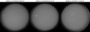 |
Fig. A.1. GONG Hα images of ARs NOAA 12740 (left panel), NOAA 12706 (middle panel), and NOAA 12738 (right panel). Around the three ARs the fibrils observed in the Mg II h3 mosaic are glimpsed. No other structures, such as filaments or filament channels, are observed. Data were acquired by the GONG instruments hosted by Learmonth Solar Observatory and Udaipur Solar Observatory, operated by the National Solar Observatory Integrated Synoptic Program (NISP). |
Appendix B: Mg II h fibrils
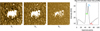 |
Fig. B.1. Closeup view of AR NOAA 12706 and its surroundings in the Mg II h non center-to-limb corrected mosaic at different spectral pixels, i.e., from left to right, at the 50th, 54th, and 63th spectral points, corresponding respectively to the h3, h2r, and h1r in the full-disk mean line profile (right panel). North is up and west is to the right. The FoV has dimensions 500″ × 410″. It is possible to notice a downward trend in the visibility of fibrils when moving away from h3. |
Appendix C: Center-to-limb variations
In our case, the center-to-limb effects are expected to be relevant in the average intensity measurements only for the CH and the coronal DH, since the QS and the fibrillar DH are at a similar radial distance from the disk center.
Different center-to-limb effects are evident in all IRIS mosaics and AIA filtergrams. Mg II h&k lines are known to present limb darkening (e.g., Morrill & Korendyke 2008), which has been measured in IRIS mosaics by Gunár et al. (2021). These authors find that the amplitude of the limb darkening decreases with the wavelength range used for the integration. As a consequence, we would not expect to find this effect in the h3 or k3 full disks. However, we find a non-negligible limb darkening in the h3 and k3 mosaics. All other IRIS mosaics and AIA filtergrams (except for AIA 304 Å) show instead more or less obvious center-to-limb brightening, with the Si IV mosaics and the hotter AIA bands being the most conspicuous.
We chose to correct these variations through a standardized empirical method that takes into account the center-to-limb trend of each waveband or wavelength. The observed intensity, Iobs(μ ), for each line or band, as a function of μ, the cosine of the heliocentric angle, θ, is a function of the intensity observed at the disk center, I(μ =1 ), and hence is not modified by line-of-sight effects. This function is expressed with the factor, fλ(μ), which is different for each line or band:
 (C.1)
(C.1)
Therefore, knowing fλ(μ) it is possible to obtain the intensity, Iλ(μ = 1), corrected for the center-to-limb effects.
To retrieve the factor, fλ(μ), for each IRIS line and AIA waveband we used seven dates of minimum of solar activity (March 26, 2018, September 24, 2018, October 23, 2018, September 22, 2019, October 20, 2019, February 23, 2020, and March 23, 2020) to characterize the dependence of the intensity from the radial distance. Following an approach similar to that reported in Andretta & Del Zanna (2014), we computed the bidimensional histogram of intensities as a function of μ in each annulus of size Δμ = 0.02, starting from the disk center. We excluded from the calculation all pixels with |Y|< 0.85 R⊙ in order to minimize the contribution of polar CHs that would otherwise affect the QS profile, above all during the minimum of solar activity. Then we evaluated the peak intensities averaged on the seven dates for each IRIS line and AIA band.
Then, we fit the logarithm of these peak intensities as a function of μ with a cubic function:
 (C.2)
(C.2)
so that the factor, fλ(μ), could be simply computed from the following equation:
 (C.3)
(C.3)
The fits of the seven QS day average peak-intensity curves that we obtain for IRIS lines and AIA bands are shown in blue in Fig. C.1, overplotted on the bidimensional histograms as a function of μ for the April 22, 2018 date (i.e., the AR NOAA 12706 date). Only AIA 94 Å is not shown because its plot is very similar to the AIA 335 Å one. The red lines are the measured positions of the intensity peaks of the histograms. The cubic function fits the observed average center-to-limb variation of intensities very well. The seven QS C II and Si IV mosaics used to compute fλ(μ) were obtained through the line integral. Then, the center-to-limb correction was applied to each wavelength of the April 22, 2018 C II and Si IV datacubes under the assumption of an optically thin line, which is confirmed by the limb brightening found and shown in Fig. C.1.
 |
Fig. C.1. Bidimensional histograms vs. μ are shown for all April 22, 2018 IRIS mosaics (left panels) and AIA filtergrams (right panels) used in the analysis. Each red point is the mode of the histogram in the interval Δμ = 0.02. The blue curve is the fit obtained from the seven QS dates, as described in the appendix. |
All Tables
Si IV 1393 Å Gaussian fit parameters inside the fibrillar DH, the coronal DH, the CH, and the QS.
All Figures
|
Fig. 1. From left to right: IRIS Mg II h core full-disk mosaic, AIA 171 Å and 193 Å images from April 13, 2019 (top panels) and May 5, 2019 (bottom panels), when the ARs NOAA 12738 and 12740, respectively, were on the disk. These two examples show the appearance of the DHs at the disk center and the solar limb, respectively. DHs are dark areas best seen in TR or low corona lines, such as Fe IX in the AIA 171 Å waveband. In the chromosphere, such as in Mg II h&k line cores, fibrils are often observed right next to the AR cores. |
| In the text | |
|
Fig. 2. IRIS Mg II h3 full-disk mosaic and AIA full-disk images showing the DH surrounding AR NOAA 12706 in the northern hemisphere on April 22, 2018. The three images are center-to-limb corrected. Left panel: the three fibrillar DH contours are shown in shades of green and the outer AR-core edge is shown in red. Middle and right panels: AIA 171 and 193 Å filtergrams, respectively, taken at 19:24 UT. The three coronal DH contours are shown in shades of violet in the AIA 171 Å image, while the QS box and the three southern CH contours are shown in white and in shades of blue, respectively, in the AIA 193 Å image, as described in Sect. 3. The contours are obtained through intensity thresholds from the non center-to-limb corrected images. |
| In the text | |
|
Fig. 3. C II 1334 and 1335 Å (upper panels) and Si IV 1393 and 1403 Å (lower panels) average profiles for QS, fibrillar and coronal DH and CH, in red, green, violet, and cyan respectively, with corresponding normalized histograms of the integrated intensities. The vertical dotted lines in the profiles represent the QS reference wavelengths. The yellow and gray bands identify the spectral intervals used for C II and Si IV intensity and background evaluation, respectively. In the lower left panels, the dashed curves are the Si IV 1393 Å fits. |
| In the text | |
|
Fig. 4. Closeup view of NOAA 12706 and its surroundings. From top to bottom: IRIS Mg II h3, Si IV 1393 Å, and C II 1334 Å. North is up and west is to the right. The FoV has dimensions 440″ × 410″. In the Mg II h3 it is possible to observe around the AR core the chromospheric DH made up of fibrils that have a maximum length approximately half the size of the AR in the longitudinal direction. In the C II and Si IV mosaics, instead, a halo of reduced emission is still recognizable around the AR, but less clearly and without the evident presence of fibrillar structures. |
| In the text | |
|
Fig. 5. AIA closeup views of NOAA 12706 and its surroundings. North is up and west is to the right. The FoV has dimensions 700″ × 620″. |
| In the text | |
|
Fig. 6. DH (in green) and southern CH (in blue) average intensity ratios in IRIS lines and AIA filters. The shaded areas are the ratio uncertainties, computed as discussed in Sect. 3. The chromospheric fibrillar and the 171 Å coronal DH contours were employed for the IRIS and AIA ratios, respectively. |
| In the text | |
|
Fig. 7. Average log EM curves as functions of log T calculated over the QS, coronal DH, and southern CH. The DH and the CH show a similar depletion in EM compared to the QS in the 5.6–5.9 log T range. At higher temperatures the CH exhibits a trend opposite to that of DH and QS, with a strong EM reduction. |
| In the text | |
|
Fig. 8. Average signed (top panel) and unsigned (bottom panel) magnetic field strength ∼30 min time evolution inside the four RoIs. The colored bands are the uncertainties. |
| In the text | |
|
Fig. 9. Averaged QS-subtracted histograms of the four RoIs. The gray band corresponds to the noise interval, [−8,8] G, that was cut to obtain the magnetic field strength measurements shown in Fig. 8. |
| In the text | |
|
Fig. A.1. GONG Hα images of ARs NOAA 12740 (left panel), NOAA 12706 (middle panel), and NOAA 12738 (right panel). Around the three ARs the fibrils observed in the Mg II h3 mosaic are glimpsed. No other structures, such as filaments or filament channels, are observed. Data were acquired by the GONG instruments hosted by Learmonth Solar Observatory and Udaipur Solar Observatory, operated by the National Solar Observatory Integrated Synoptic Program (NISP). |
| In the text | |
|
Fig. B.1. Closeup view of AR NOAA 12706 and its surroundings in the Mg II h non center-to-limb corrected mosaic at different spectral pixels, i.e., from left to right, at the 50th, 54th, and 63th spectral points, corresponding respectively to the h3, h2r, and h1r in the full-disk mean line profile (right panel). North is up and west is to the right. The FoV has dimensions 500″ × 410″. It is possible to notice a downward trend in the visibility of fibrils when moving away from h3. |
| In the text | |
|
Fig. C.1. Bidimensional histograms vs. μ are shown for all April 22, 2018 IRIS mosaics (left panels) and AIA filtergrams (right panels) used in the analysis. Each red point is the mode of the histogram in the interval Δμ = 0.02. The blue curve is the fit obtained from the seven QS dates, as described in the appendix. |
| In the text | |
Current usage metrics show cumulative count of Article Views (full-text article views including HTML views, PDF and ePub downloads, according to the available data) and Abstracts Views on Vision4Press platform.
Data correspond to usage on the plateform after 2015. The current usage metrics is available 48-96 hours after online publication and is updated daily on week days.
Initial download of the metrics may take a while.